Multi-objective Robust Optimization using a Post-optimality Sensitivity Analysis Technique: Application to a Wind Turbine Design
Abstract
Toward a multi-objective optimization robust problem, the variations in design variables and design environment parameters include the small variations and the large variations. The former have small effect on the performance functions and/or the constraints, and the latter refer to the ones that have large effect on the performance functions and/or the constraints. The robustness of performance functions is discussed in this paper. A post-optimality sensitivity analysis technique for multi-objective robust optimization problems is discussed and two robustness indices are introduced. The first one considers the robustness of the performance functions to small variations in the design variables and the design environment parameters. The second robustness index characterizes the robustness of the performance functions to large variations in the design environment parameters. It is based on the ability of a solution to maintain a good Pareto ranking for different design environment parameters due to large variations. The robustness of the solutions is treated as vectors in the robustness function space, which is defined by the two proposed robustness indices. As a result, the designer can compare the robustness of all Pareto optimal solutions and make a decision. Finally, two illustrative examples are given to highlight the contributions of this paper. The first example is about a numerical problem, whereas the second problem deals with the multi-objective robust optimization design of a floating wind turbine.
design variable vector
vector of design environment parameters
the th constraint
performance function vector
feasible set
Pareto optimal set
standard deviation
expected value
robustness index against small variations
feasibility index of a solution
Pareto optimality index of a solution
probability density function of
individual’s ranking
number of discrete values of design environment parameters
robustness index against large variations
the most robust solutions amongst the Pareto optimal solutions
produced power of wind turbine rotor
the thrust force in the partial load region of a wind turbine rotor
the root twist angle
the tip twist angle
the chord length at the root
the chord length at the tip
rotor rotational speed
root radius of the wind turbine
tip radius of the wind turbine
number of blades
air density
reference wind speed
HAWT Horizontal Axis Wind Turbine
MOOP Multi-Objective Optimization Problem
MOROP Multi-Objective Robust Optimization Problem
RIRobustness Index
RDPRobust Design Problem
RF-SpaceRobustness Function Space
DV Design Variable
DEP Design Environment Parameter
PF-SpacePerformance Function Space
PDFProbability Density Function
BEMTBlade Element Momentum Theory
UDUniform Distribution
NDNormal Distribution
N/ANot Affected
1 Introduction
Many design optimization problems are Multi-Objective Optimization Problems (MOOP) and are subject to uncertainties or variations in their parameters. Robustness is a product’s ability to maintain its performance under the variations in its parameters. Robust design aims at maximizing product’s robustness. In other words, it aims at minimizing the sensitivity of performance to variations without controlling the source of these variations [1]. Sometimes, the robustness of a product is as important as or even more important than its performance. So, to focus on the trade-off between robustness and performance of a product is meaningful. For such problems, namely Multi-Objective Robust Optimization Problems (MOROP), it is important to obtain design solutions that are both optimal and robust.
There exist some Robustness Indices (RI) for MOROP in the literature. In fact, how to account for the variations in design parameters and how to measure robustness is a widely discussed problem [2]. Without loss of generality, the design parameters can be divided into two types, Design Variables (DVs), which can be controlled by the designer, and Design Environment Parameters (DEPs), which are uncontrollable parameters.
Existing works mainly focus on the small variations in DVs and DEPs [3, 4, 5, 6, 7, 8, 9, 10, 1, 11, 12, 13, 14, 15, 16, 17, 18, 19]. Moreover, some previous work focused on the variations in the performance function model [20, 21, 22, 23]. Toward MOOP, the designer’s preference is also a type of variation in MOROP [24, 25, 26].
Besides the small variations in DVs and DEPs, there may be large variations in DEPs in some engineering problems. For instance, the actual wind speed may vary greatly in a short time for a wind turbine rotor. In some areas, the environment temperature can fluctuate greatly between daytime and night. As a matter of fact, the problem with regard to large variations in DEPs can be considered as a special dynamic optimization problem, where the performance function and/or the constraints change with time [27, 28, 29, 30, 21, 22].
One way to distinguish between small variations and large variations in design parameters is whether they are uncertain or not [31]. Another way to distinguish between small and large variations is whether a linearization is reasonable over the range of variations. The distinction between small and large variations is commonly presented as local versus global sensitivity analysis in the literature on sensitivity analysis [32, 33, 34, 35]. The concept of large variations has been discussed in [36, 16, 23, 37] for comparing the difference between the linear and nonlinear performance functions. Nevertheless, in those discussions with regard to large variations, most of the existing criteria for MOROP aim at finding a design solution that gives desirable means, variances, quantiles or probabilities of violating constraints based on the distributions of the performance and constraint values with respect to the variations in the design parameters. Few criteria aim at finding a solution that maintains a good Pareto ranking for as many different DEP values in the sample space as possible. As a matter of fact, the Pareto ranking of a solution may be dramatically affected due to large variations in DEPs. In this paper, the distinction between small are large variations is made based on their effect on the performance functions. The small variations in design parameters refer to the ones that have small effect on the performance functions. The large variations in design parameters refer to the ones that have large effect on the performance functions.
Accordingly, a post-optimality sensitivity analysis technique for multi-objective robust optimization problems is discussed while considering both small and large variations in design parameters. Two robustness indices (RI) are also introduced. The first one characterizes the robustness of MOOPs against small variations in the design parameters. It is based on the distributions of the performance function values with respect to these small variations. The second robustness index characterizes the robustness of MOOPs against large variations in DEPs. It is based on the solution’s ability to maintain a good Pareto ranking for as many different design environments as possible. As a result, the designer can make a decision based on the robustness of the solutions.
The paper is organized as follows. Section 2 provides the theoretical background on Multi-Objective Optimization Problems (MOOPs), Robust Design Problems (RDPs) and Multi-Objective Robust Optimization Problems (MOROPs). Two Robustness Indices (RI) and the concept of Robustness Function Space (RF-Space) are introduced in Section 3. Two illustrative examples are given in Section 4 to highlight the contributions of the paper. The first example is about a numerical problem, whereas the second problem deals with the multi-objective robust optimization design of a floating wind turbine. Conclusions and future work are presented in Section 5.
2 Theoretical Background
2.1 Multi-Objective Optimization Problem
A general formulation of MOOP is given in Eqn. (1):
| (1) |
where denotes the -dimensional vector of performance functions. denotes the -dimensional vector of DVs. Note that the nominal values of DV are controllable, and are the lower and upper bounds of respectively. denotes the -dimensional vector of DEP, which cannot be adjusted by the designer, and they are uncontrollable parameters. The functions are the constraints. A design that does not violate any constraint is called “feasible”. The set of feasible solutions is called feasible set and named .
Since there are some trade-offs amongst the conflicting objectives, none solution of can dominate another solution of . The optimization problem (1) generally has more than one optimal solutions. Those solutions are defined as Pareto optimal solutions, which cannot be dominated by any other feasible solution [38, 39, 40, 26]. The set of all Pareto optimal solutions is called Pareto optimal set and named . The Pareto optimal solutions lie on a boundary in the Performance Function Space (PF-Space), called Pareto front.
2.2 Robust Design Problem
The concept of robustness is used in many fields such as engineering, biology, economy, computer science [41, 42, 26, 43, 44, 45, 46, 47]. In this paper, the robustness of a product is defined as follows:
Definition 1
Robustness is a product’s ability to maintain its performances under conditions of varying parameters.
Robust design, a term originally introduced by Genichi Taguchi [48], is a way of improving the quality of a product by minimizing the effect of variations, without eliminating the causes themselves. Many researchers refer to robustness [49, 50, 51, 52, 1, 53, 54, 55, 56].
Although different expressions are used, their meanings are similar. In this paper, we define the robust design as follows:
Definition 2
The design of a product is robust if and only if the performances of the good under design is as little sensitive as possible to variations and uncertainties.
2.3 Multi-Objective Robust Optimization Problem
A MOROP aims to find out a solution that is feasible, optimal and robust. To come up with an feasible, optimal and robust design, the three following scenarios have been identified.
-
1.
Optimal design and robust design are equally important: It means that performance functions and robustness functions are optimized simultaneously. The designer can use the new performance functions by adding the effects of robustness, instead of original performance functions [3, 4, 6, 7, 57]. Moreover, the robustness functions can be considered as new constraints [8, 9, 58, 59, 14, 16, 17, 60] or additional optimization objectives [15, 61, 62, 63, 64, 65, 66, 67].
- 2.
-
3.
Robust design is primary and optimal design is secondary: The final solution is selected from the most robust solutions based on the values of the performance functions [12].
In this paper, the optimal design is supposed to be of primary importance and the robust design of secondary importance. Although there exist some papers dealing with this method [68, 69, 70, 24, 25, 71, 18, 19, 72], which is also called as post-optimality sensitivity analysis, the final solution is selected from the Pareto optimal set based on its robustness. Moreover, in this paper we consider both small variations in design parameters and large variations in DEPs simultaneously.
3 New Robustness Indices for MOROP
Two Robustness Indices (RI) are introduced in this section. Then, the concept of RF-Space is presented and the solution robustness is defined as a vector in the RF-Space. Finally, a discussion on this new method is presented.
3.1 Robustness Index with regard to the Small Variations in DVs and DEPs
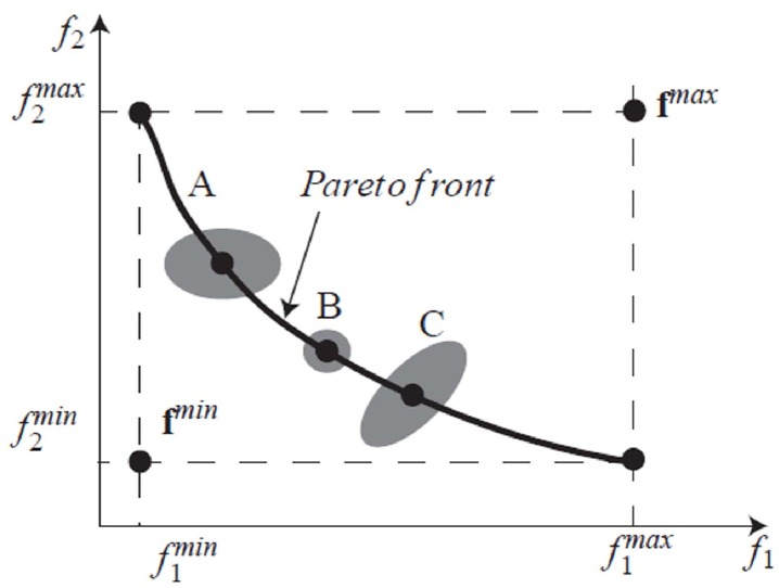
Figure 1 illustrates the solutions of a simple multi-objective optimization problem. It has two performance functions (,,), some DVs () and DEPs (). Let us select solution A, solution B and solution C, which are located on the Pareto front. When there are small variations in DVs and DEPs, then their performances varies in the grey area around their nominal values in the PF-Space, as shown in Fig. 1. Obviously, in the PF-Space, solution B has smaller variations around its nominal values than solutions A and C. It means than solution B is more robust than solutions A and C. However, the size of the grey areas associated with solution A and solution C are the same, but their shapes are different. So the comparison between the robustness of solution A and solution C is not an easy task. Toward the different types of uncertainties, there are different methods to define RI for MOOP, such as using the worst case scenario [14, 15, 16, 73, 17], the expectancy measure [6, 7, 3, 4, 5, 8, 9, 49, 2, 74], and the probabilistic threshold method [8, 9, 2].
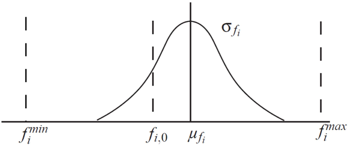
We select a RI against the small variations in DVs and DEPs, based on the expectancy measure. A new RI () is introduced and is based on the actual variations of performances. Under the small variations in DVs and DEPs, the actual performances are distributed around the nominal values. In the PF-Space, the actual performances follow a multivariate distribution. Here, in order to simplify the index associated with each performance function, the standard deviation of the actual performances is used as a measure for the robustness: the smaller the standard deviation, the more robust the design. The absolute value of the difference between the expected value () and the nominal value () is also a robustness measure: the smaller the absolute difference, the more robust the design. Figure 2 shows an example, which follows a normal distribution, and are the standard deviation and expected value of the th performance function under small uncertainties; is the nominal value; and are the maximum and the minimum values of the th performance function on the Pareto front, respectively.
Here, we assume that the standard deviation () and the absolute value of the difference between and have the same importance for the designer. Moreover, we assume that the robustness of all performance functions has the same importance. The robustness index of a MOOP with respect to small variations in DVs and DEPs is defined as a scalar. The robustness of each performance function is also normalized. To normalize the sum of the standard deviation () and the absolute difference (), we divide it by the difference between the two extreme values of the th performance function, namely, . As a result, is defined as follows:
| (2) |
The smaller , the more robust the design.
Note that even if the variations are small, the constraints may not be satisfied due to variations. This refers to the robustness of constraints (reliability). As a matter of fact, the index is not discussed deeply in this paper. It is just based on the distributions of the performance function values with respect to these small variations. To simplify the index, the reliability with regard to small variations is not considered in this paper.
3.2 Robustness Index with regard to the Large Variations in DEPs
Since the DVs are controllable and the DEPs are uncontrollable, we assume that there are only large variations in DEPs. The mapping functions between the DVs and performance functions can change a lot due to large variations in DEPs. For a MOOP while considering large variations in DEPs, we assume that the initial DEPs are , the set of feasible solutions is named and the set of Pareto optimal solutions is denoted . It is noteworthy that those Pareto optimal solutions are alternative solutions for the designer.
Since large variations in DEPs exist, the DEPs may change from to . The design environment parameters are supposed to take discrete values: . The Probability Density Functions (PDF) of are . The initial DEPs are equal to the ones having the maximum PDF amongst the discrete values. The corresponding feasible sets are . A feasible and Pareto optimal solution in may not be Pareto optimal, and not feasible in the new environments. To compare the solution’s robustness against large variations in DEPs, the traditional methods are not applicable. Toward a MOOP, a definition of the solution’s robustness against large variations in DEPs is proposed thereafter:
Definition 3
Toward a multi-objective optimization problem against large variations in DEPs, solution’s robustness against large variations in DEPs is a measure of its ability to be optimal in different design environments.
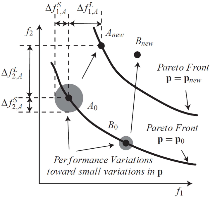
Figure 3 illustrates the solutions of a simple MOOP. Similarly to Fig. 1, the problem has two objective functions (,), some DVs () and DEPs (). is the nominal values of DEPs. Let us consider Pareto-optimal solutions and as examples. The grey area shows the variations in performances of solution and solution in the PF-Space, under small variations in DVs and DEPs. As seen before, we can conclude that solution is more robust than solution with regard to small variations in DVs and DEPs.
On the contrary, it may not be the case if there are large variations in DEPs. As shown in Fig. 3, in a new environment, we assume that when the DEPs change from to , there are large variations in the PF-Space for all the solutions. For instance, in the PF-Space, solution A moves from to , solution B moves from to . Both solutions have quite large variations in . Then, the following question remains: “How can we compare the robustness of solutions and ”?.
As shown in Fig. 3, toward solution , and represent the largest distance of the actual performance function values and nominal performance function values in and respectively, with regard to the small variations in DVs and DEPs. and represent the largest distance of the actual performance function values (assuming only two samples: and ) and nominal performance function values in and respectively, with regard to large variations in DEPs. If , , and , , we can see that the caused actual performance function values of both solution and solution are sufficiently far from their nominal ones, with regard to large variations in DEPs. As a consequence, we can conclude that the traditional methods, which provide some results based on the difference between actual performance function values and nominal ones, make little sense. Therefore, the method proposed in this paper aims to compare their relative positions in the PF-Space associated with the new environment. From Figure 3, we can see that, in the new environment, , solution is still on the new Pareto front, which means that it is still one of the best solutions for the designer. Meanwhile, solution is far away from the new Pareto front, which means that it is no longer a good choice for the designer. As a result, we can conclude that solution is more robust than solution with regard to the large variations in DEPs.
As a result, a RI with regard to large variations in DEPs is defined thereafter. Toward the discrete probability distribution of DEPs, mathematically, the RI of a solution is defined as follows:
| (3a) | |||
| (3d) | |||
| (3e) | |||
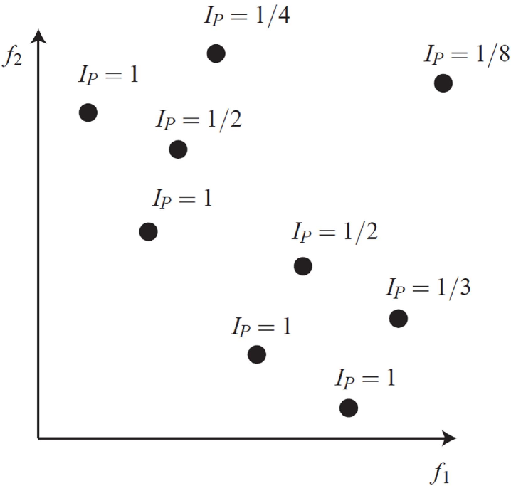
where is the Feasibility Index of the solution; is the Pareto optimality Index of the solution; is the PDF of ; is the individual’s ranking in the new environment where and amounts to the number of individuals by which it is dominated amongst the alternative solutions, plus one [75, 76]. For a better understanding, a simple example is shown in Fig. 4. In a new environment, if a solution is still non dominated by any other solution, then the value will be equal to one for that solution. Otherwise, the value will be lower than one, but greater than zero. Note that the number of the alternative solutions affects the value. However, the proposed definition can divide the alternative solutions into different groups based on their robustness.
Note that the index is bounded between zero and one. On the one hand, if a solution is feasible in all environments and cannot be dominated by any other solution in all possible environments, then . On the other hand, if a solution is non-feasible in some new environments, then . If each solution belongs to the set of Pareto optimal solutions , then if it is feasible in all environments and its value will be greater than or equal to zero and smaller than one.
Note that the individual’s ranking corresponds to a specific value of DEPs: , where . In case there exist continuous probability distributions of the DEPs, becomes infinite and it is difficult to assess the robustness index for a solution . However, since the domain of the DEPs can be partitioned into many small parts, we can simplify such a problem by using a discrete probability distribution of the DEPs.
Finally, the smaller , the more robust the design with regard to large variations in DEPs.
3.3 Robustness Function Space
In this paper, we consider not only the RI against small variations, , but also the RI against large variations, . The RI of a Pareto-optimal solution is represented as a vector. The designer can analyze the robustness of Pareto optimal solutions in the Robustness Function Space (RF-Space). For a better understanding, we take as one dimension of the RF-Space, another dimension of the RF-Space is , as shown in Fig. 5.
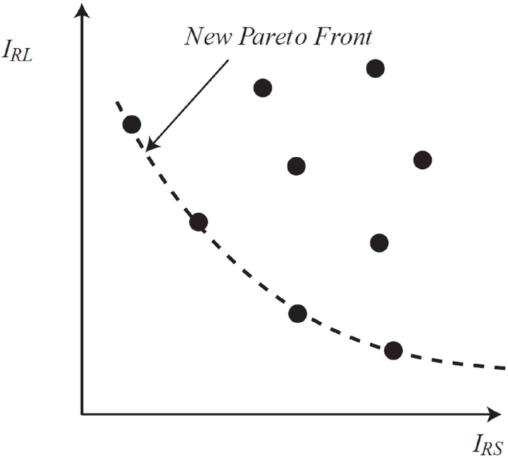
Thanks to the proposed method, each Pareto optimal solution has a corresponding position in the RF-Space, as shown in Fig. 5. If and are not conflicting, then the designer will be able to select the most robust solution immediately, namely, the solution that minimizes both and . If and are two conflicting objectives, then a new Pareto front in the RF-Space will appear. The Pareto-robust solutions represent the most robust solutions amongst the Pareto optimal solutions. The set of Pareto-robust solutions is named . Finally, the designer can select the final solution from this set according to his/her requirements.
3.4 Flow chart
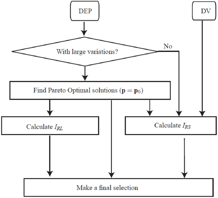
A flow chart is illustrated in Figure 6 for a better understanding of the proposed post-optimality sensitivity analysis technique. The first step is to determine whether the design environment parameters (DEP) are subject to large variations or not. The distinction between small and large variations is made with regard to their effect on the performance functions. The small variations in design parameters refer to the ones that have a small effect on the performance functions. The large variations in design parameters refer to the ones that have large effect on the performance functions. In the second step, Pareto optimal solutions are obtained for different values of DEP. Those different values of DEP are due to large variations in DEP. In the third step, robustness indices and are calculated for each solution. The new Pareto ranking of the obtained Pareto optimal solutions are obtained in different design environments. Finally, the designer can make a decision from the obtained Pareto optimal solutions based on their robustness, namely, based on the values of and for each solution.
4 Examples
In this section, two illustrative examples are given in order to highlight the contributions of the proposed approach. The first example is a simple numerical example and the second example is a MOROP of a wind turbine blade design, in which the variations include not only the small variations in DVs and DEPs, but also large variations in DEPs.
4.1 Numerical illustrative example
The problem is defined in Eqn. (4). There are two performance functions and , one design variable , one design environment parameter and one constraint:
| minimize | (4a) | ||||
| minimize | (4b) | ||||
| subject to | (4c) | ||||
| (4d) | |||||
is subject to small variations and the variations in follow a uniform distribution and are bounded between and . is subject to large variations and can take three possible values: , and . The probabilities for to take those three values are , and , respectively. The initial value of is equal to 5.
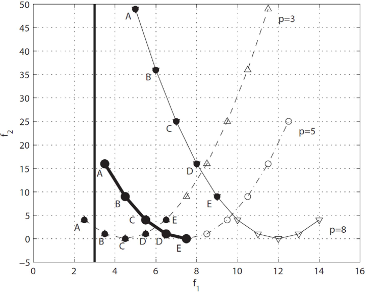
Figure 7 shows the values of the performance functions and for , and , respectively, i.e., in different design environments. For , let us consider the five Pareto optimal solutions: solution A obtained for ; solution B obtained for ; solution C obtained for ; solution D obtained for and solution E obtained for . These solutions form the Pareto front in the PF-Space and are alternative solutions for the designer. Their new positions for and in the PF-Space are shown in Fig. 7. The vertical line represents the constraint related to the first performance function. Note that the solutions to the right of this line are feasible, whereas the solutions to the left are not feasible.
To assess the robustness index for each alternative solution, the samples around the nominal values are generated by Latin Hypercube Sampling (LHS) [77, 78, 79]. 1000 samples for each alternative solution are generated with regard to the small variations in DV. Then for each alternative solution can be assessed with Eqn. (2).
To determine the robustness index associated with each alternative solution, their new positions should be located when changes from its initial value to its new value. The results can be found from Fig. 7. When , solution A becomes unfeasible, then the index defined in Eqn. (3d) is null for solution A. Solution B and solution C become Pareto optimal amongst these five solutions. Solution D and Solution E are dominated by other alternative solutions. When , all the alternative solutions are feasible and can not be dominated by others. Then for each alternative solution can be calculated with Eqn. (3).
| Solution | ||||||
|---|---|---|---|---|---|---|
| A | 3.5 | 16 | 0.05 | 0.4024 | 1.5 | 33 |
| B | 4.5 | 9 | 0.05 | 0.3024 | 1.5 | 27 |
| C | 5.5 | 4 | 0.05 | 0.2024 | 1.5 | 21 |
| D | 6.5 | 1 | 0.05 | 0.1025 | 1.5 | 15 |
| E | 7.5 | 0 | 0.05 | 0.0025 | 1.5 | 9 |
Note that all Pareto optimal solutions have sufficiently large variations in performance functions with regard to large variations in DEPs. In Tab. 2, and denote the nominal values of the performance functions for the alternative solutions. and represent the largest distance of the actual performance function values (1000 samples for each alternative solution) and nominal performance function values in and respectively, with regard to the small variations in DV. and represent the largest distance of the actual performance function values (3 samples for each alternative solution) and nominal performance function values in and respectively, with regard to large variations in DEP. If the traditional methods (results based on the difference between actual performance function values and nominal ones) are selected to measure the robustness of the alternative solutions, here is the order of the six solutions from the most robust one to the least robust one: (1) E; (2) D; (3) C; (4) B; (5) A. Even if solution E is the most robust one, and are still quite large. Obviously, and , so with regard to large variations in DEPs, the traditional methods make little sense.
Here is the order of the six solutions from the most robust one to the least robust one while using the robustness index defined in Eq. (3a): (1) B; (1) C; (3) D; (4) E; (5) A. Solution B and solution C are Pareto optimal no matter the value of DEP . Therefore, the designer may select solution B or solution C instead of solution E.
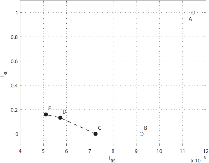
Figure 8 illustrates the positions of the alternative solutions in the RF-Space. In this space, one dimension is , another dimension is . In this example, and are two conflicting objectives, as shown in Fig. 8. Solutions C, D, E form a new Pareto front in the RF-Space, which represents the most robust solutions amongst these five alternative solutions. For a better understanding, the performance function values and their RIs are given in Tab. 2. The indices and are also given in Tab. 2.
| Solutions | ||||||||
|---|---|---|---|---|---|---|---|---|
| A | 3.5 | 16 | 0.0115 | 0 | 1 | 1 | 1 | 1 |
| B | 4.5 | 9 | 0.0092 | 1 | 1 | 1 | 1 | 0 |
| C | 5.5 | 4 | 0.0072 | 1 | 1 | 1 | 1 | 0 |
| D | 6.5 | 1 | 0.0057 | 1 | 0.3333 | 1 | 1 | 0.1333 |
| E | 7.5 | 0 | 0.0051 | 1 | 0.2 | 1 | 1 | 0.16 |
Thanks to the proposed method, the designer can select the final solution from the new Pareto front in the RF-Space, according to his/her requirement. For example, if the designer prefers the index, solution E will be selected. If the designer prefers the index, solution C will be selected.
4.2 Multi-Objective Robust Optimization Design of a Floating Wind Turbine
4.2.1 Problem Formulation
Figure 9 illustrates a schematic of a floating horizontal wind turbine rotor with two simplified morphing blades. Each blade can adjust its tip twist angle and root twist angle according to the reference wind speed [80]. However, it is difficult to adjust the twist angles at all time. Therefore, the twist angle is assumed to be adjusted according to the average wind speed. After setting the tip twist angle () and root twist angle (), the twist angles of the other elements are adjusted automatically and they are linearly distributed along the blade.
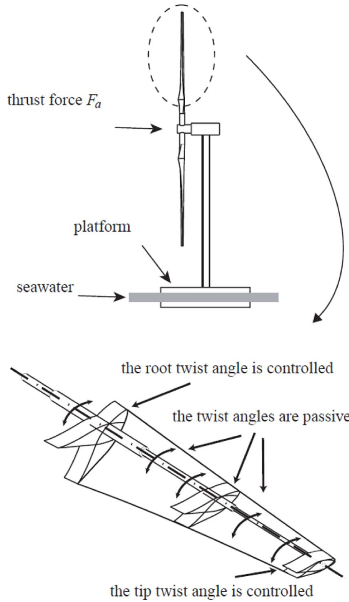
The optimization problem at hand has two objective functions: the produced power by the wind turbine that should be maximized and the thrust force that should be minimized. Moreover, the produced power should be higher than 1 kW and lower than 25 kW.
and are calculated based on the Blade Element Momentum Theory (BEMT) knowing the design parameters. A simplified morphing blade with a constant profile type (S809) along the span is used. For more details, the reader is referred to [80].
To make a good comparison, we take an optimum result as a reference blade, and its parameters are the initial design parameters [80]. The sum of the root chord length and the tip chord length is supposed to be constant and equal to . Then the four DVs are: () the root twist angle ; () the tip twist angle ; () the chord length at the root ; () the rotor rotational speed . The initial values, the lower and upper bounds of the DVs are given in Tab. 3.
| DV | Initial Value | Minimum | Maximum | Noise values |
|---|---|---|---|---|
| root twist angle (deg) | 22.8 | 0 | 35 | ( UD) |
| tip twist angle (deg) | 3.61 | -5 | 15 | ( UD) |
| root chord length (m) | 0.737 | 0.595 | 0.895 | ( UD) |
| rotor rotational speed (rpm) | 72 | 40 | 100 | ( UD) |
The other design parameters, such as the number of blades (), tip radius (), root radius (), air density () and reference wind speed () are taken as DEPs. Their nominal values are fixed as shown in Tab. 4.
| DEP | Value | Noise |
| number of blades b | 2 | N/A |
| tip radius (m) | 5 | ( UD) |
| root radius (m) | 1.27 | ( UD) |
| air density | ( UD) | |
| reference wind speed (m/s) | 10 | ( ND) |
A MOOP is formulated as follows:
| minimize | (5a) | ||||
| minimize | (5b) | ||||
| over | (5c) | ||||
| (5d) | |||||
| subject to | (5e) | ||||
| (5f) | |||||
| (5g) | |||||
| (5h) | |||||
| (5i) | |||||
| (5j) | |||||
| (5k) | |||||
For HAWTs, the variations in DVs and DEPs are unavoidable. Here, we assume that there are noise values in DVs and DEPs, as shown in Tables 3 and 4. Most of them are small variations. However, the noise values in reference wind speed (the performance functions are functionally dependent on it) is quite large, compared with its nominal value. The noise values of small variations are supposed to be Uniform Distribution (UD). The noise values of the reference wind speed follow a Normal Distribution (ND) and the corresponding standard deviation is equal to .
4.3 Results Analysis
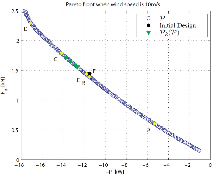
According to the proposed method, the final solution comes from the Pareto optimal set. In this paper, the Pareto optimal solutions are obtained by using the genetic algorithm (NSGA II [81]). The obtained Pareto front for this problem is illustrated in Fig. 10, including 200 alternative solutions.
To assess the robustness index for each alternative solution, the samples around the nominal values are generated by Latin Hypercube Sampling (LHS) [77, 78, 79]. 1000 samples for each alternative solution are generated with regard to the small variations in DVs and DEPs. Then for each alternative solution can be assessed using with Eqn. (2).
To determine the robustness index with regard to large variations in one DEP for each alternative solution, the new positions of the alternative solutions should be presented, when DEPs change from initial values to the new values. Then the feasibility index and the Pareto optimality Index of a solution can be determined.
In this problem, the wind speed has a continuous probability distribution, varying from 6 m/s to 14 m/s. To simplify the problem, we calculate the probability distribution of the wind speed, and convert it into a discrete probability distribution problem. Table 5 shows the probability distribution of the wind speed. The solution having the maximum PDF amongst the N probabilities is appointed as the initial DEPs , hence in this problem.
| 6 | 7 | 8 | 9 | 10 | 11 | 12 | 13 | 14 | |
| h(p) | 0.028 | 0.066 | 0.124 | 0.180 | 0.204 | 0.180 | 0.124 | 0.066 | 0.028 |
Figure 11 illustrates the positions of the alternative solutions in different design environments. The vertical lines represent the constraints in the first objective function, i.e., the produced power , then the solutions between the two lines are feasible. From the results, we can see that some alternative solutions are non-feasible in the new environments. They are illustrated by red crosses in Fig. 11. The index defined in Eqn. (3d) is null for those solutions. In the new environment, some alternative solutions are dominated by other alternative solutions, then their index defined in Eqn. (3e) is lower than one, but greater than zero. Then the for each alternative solution can be calculated with Eqn. (3a).
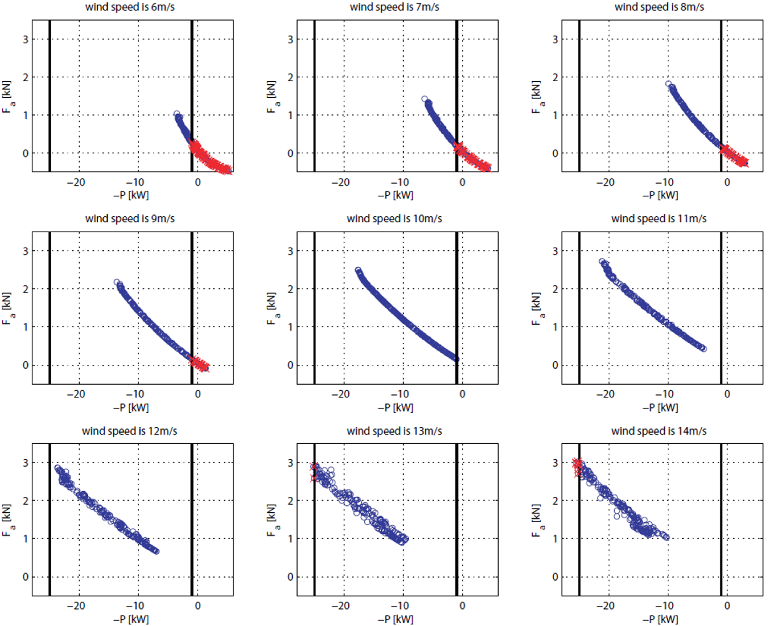
Figure 12 illustrates the positions of the alternative solutions in the RF-Space. In this space, one dimension is , another dimension is . In this example, and are two conflicting objectives, as shown in Fig. 12. A new Pareto front in the RF-Space appears, which represents the most robust solutions amongst the Pareto optimal solutions and denoted by .
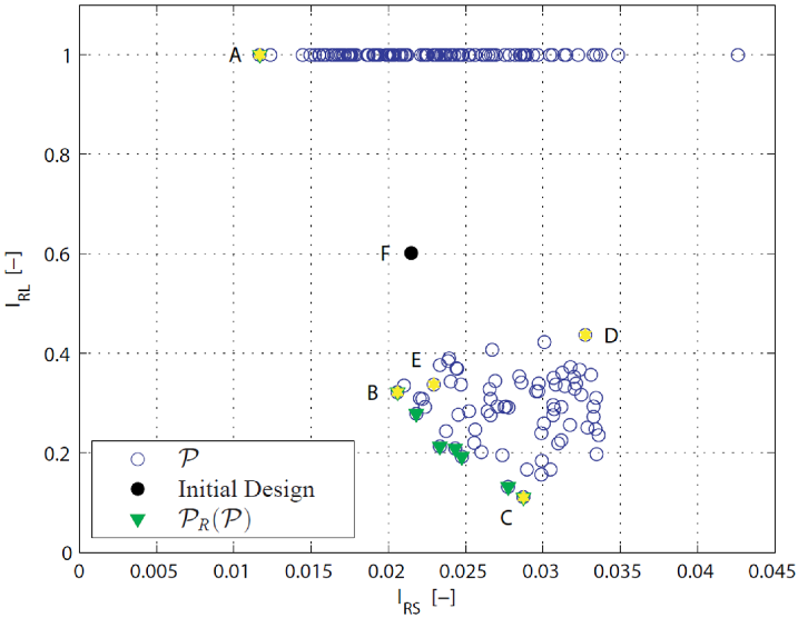
For a good understanding of the two proposed robustness indices defined by Eqn. (2) and Eqn. (3a), the six solutions A, B, C, D, E and F are selected. Their corresponding positions in the PF-Space and the RF-Space are illustrated in Fig. 10 and Fig. 12. All alternative solutions and the initial design are shown in Fig. 13. The initial design, solution F, is plotted in black and the other five solutions are plotted in yellow.
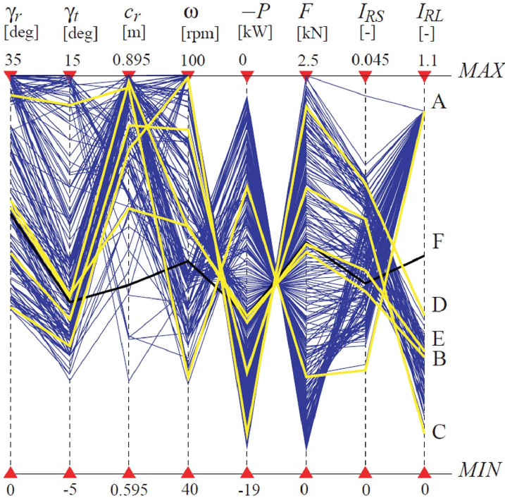
Solution A has the minimum value in the . Solution B dominates Solution F in the RF-Space. Solution C has the minimum value in the . Solution D can be dominated by many solutions such as Solutions B, C and E in the RF-Space. Solution E dominates the initial design in the PF-Space. The 3D models of the six selected solutions and the values of their DVs are depicted in Fig. 14.
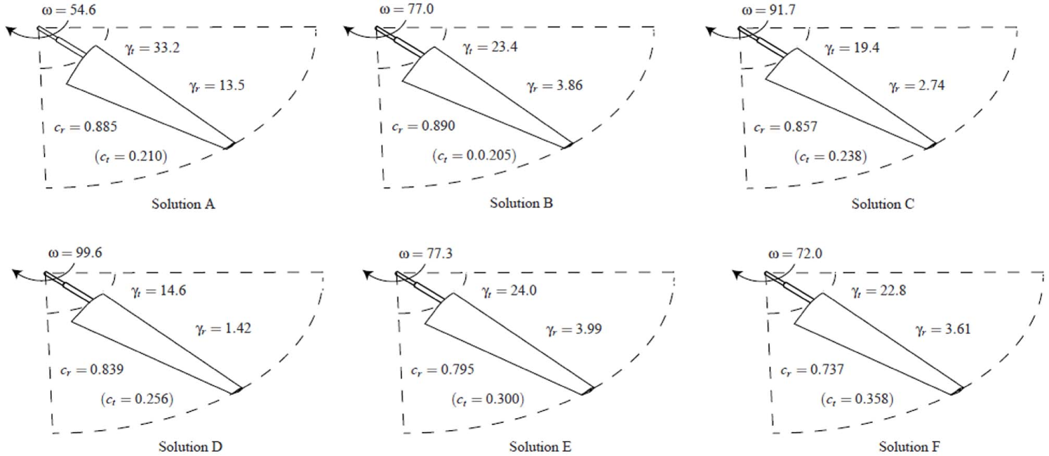
Note that the value of index of a solution depends on its ranking amongst the Pareto optimal solutions. To determine the index of the initial design, i.e., solution F, we include it into the Pareto optimal set (including 200 alternative solutions) and rank the 201 individuals to generate its ranking in different DEPs. The performance function values and the RIs for these six solutions are given in Tab. 6. For a better understanding of index , indices and of these six solutions are also given in Tab. 6.
| Solutions | - (kW) | (kN) | ||||||||||||
|---|---|---|---|---|---|---|---|---|---|---|---|---|---|---|
| A | -5.322 | 0.609 | 0.0115 | 0 | - | - | - | - | - | - | - | - | - | 1 |
| B | -11.5 | 1.399 | 0.0208 | 1 | 1 | 1 | 1 | 1 | 1 | 1/4 | 1/6 | 1/10 | 1/4 | 0.322 |
| C | -14.2 | 1.799 | 0.0287 | 1 | 1/4 | 1 | 1 | 1/2 | 1 | 1 | 1 | 1 | 1 | 0.111 |
| D | -17.1 | 2.300 | 0.033 | 1 | 1 | 1 | 1 | 1/2 | 1 | 1/4 | 1/11 | 1/13 | 1/8 | 0.437 |
| E | -11.8 | 1.444 | 0.023 | 1 | 1 | 1 | 1/2 | 1/2 | 1 | 1 | 1/7 | 1/9 | 1/3 | 0.338 |
| F | -11.5 | 1.455 | 0.0219 | 1 | 1 | 1 | 1/2 | 1 | 1/5 | 1/11 | 1/13 | 1/16 | 1/19 | 0.601 |
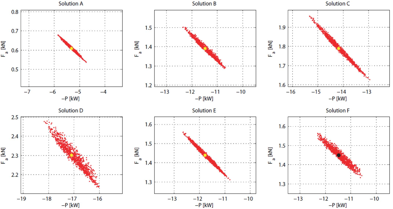
With regard to the small variations in DVs and DEPs, each solution has 1000 generated samples in the PF-Space. Figure 15 shows the samples and the nominal values of these six solutions. It is apparent that Solution A is the most robust one amongst the six solutions considering small variations in DVs and DEPs as the dispersion of the two performance functions is a minimum with regard to small variations in DVs and DEPs for this solution. It matches with their positions in the RF-Space. The robustness indices with regard to small variations for the five other solutions are given in the fourth column of Tab. 6. Here is the order of the six solutions from the most robust one to the least robust one with respect to : (1) A; (2) B; (3) F; (4) E; (5) C; (6) D.
| Solutions | (kW) | (kN) | ||||
|---|---|---|---|---|---|---|
| A | -5.32 | 0.609 | 0.576 | 0.0694 | 6.28 | 0.416 |
| B | -11.5 | 1.399 | 0.801 | 0.110 | 10.2 | 0.410 |
| C | -14.2 | 1.799 | 1.22 | 0.168 | 12.5 | 0.557 |
| D | -17.1 | 2.300 | 1.08 | 0.177 | 13.9 | 0.493 |
| E | -11.8 | 1.444 | 0.977 | 0.120 | 10.7 | 0.453 |
| F | -11.5 | 1.455 | 0.910 | 0.113 | 9.57 | 0.366 |
With regard to large variations in DEPs, all Pareto optimal solutions have sufficiently large variations in performance functions. In Tab. 7, and represent the nominal performance function values of the alternative solutions. and represent the largest distance of the actual performance function values (1000 samples for each alternative solution) and nominal performance function values in and respectively, with regard to the small variations in DVs and DEPs. and represent the largest distance of the actual performance function values (9 samples for each alternative solution) and nominal performance function values in and respectively, with regard to large variations in DEPs. The results show that and , so with regard to large variations in DEPs, the traditional methods (results based on the difference of actual performance function values and nominal ones) make little sense. On the contrary, the method proposed in this paper is relevant. Indeed, here is the order of the six solutions from the most robust one to the least robust one based on the index: (1) C; (1) B; (3) E; (4) D; (5) F; (6) A.
In summary, the designer can select the final solution from the new Pareto front in the RF-Space, according to his/her requirement. For example, if the designer prefers the , solution A should be selected. If the designer prefers the , solution C should be selected.
5 Conclusions and Future Work
In this paper, a new method for solving Multi-Objective Robust Optimization Problems (MOROP) has been introduced and two illustrative examples have been given to highlight the main contributions of the paper. Two Robustness Indices (RI) have been introduced to deal with MOROP where not only small variations in Design Variables (DVs) and Design Environment Parameters (DEPs) are considered, but also large variations in DEPs. The first robustness index, named , characterizes the robustness of MOOP against small variations in DVs and DEPs. The second robustness index, named , characterizes the robustness of Multi-Objective Optimization Problems (MOOP) against large variations in DEPs. The robustness index is calculated based on the standard deviations and the differences between the expected values and nominal values of the performances. The smaller , the more robust the design. The robustness index is calculated based on the solution’s ability to be optimal in different design environments. The smaller , the more robust the design. To make a trade-off between the two proposed robustness indices, a concept of Robust Function Space (RF-Space) has been introduced. Then each Pareto optimal solution has a position in the RF-Space. The designer can select the final solution from the Pareto optimal set based on its new position in the RF-Space. However, some problems are still not solved. For instance, it is not always an easy task to claim whether a variation is small or large. Moreover, new formulations for and should be discussed in the future.
References
- [1] Caro, S., Bennis, F., and Wenger, P., 2005. “Tolerance synthesis of mechanisms: a robust design approach”. Journal of Mechanical Design, 127, pp. 86–94.
- [2] Beyer, H., and Sendhoff, B., 2007. “Robust optimization-a comprehensive survey”. Computer methods in applied mechanics and engineering, 196(33-34), July, pp. 3190–3218.
- [3] Deb, K., and Gupta, H., 2005. “Searching for robust Pareto-optimal solutions in multi-objective optimization”. In Evolutionary Multi-Criterion Optimization, C. Coello Coello, A. Hernández Aguirre, and E. Zitzler, eds. Springer Berlin / Heidelberg, pp. 150–164.
- [4] Deb, K., and Gupta, H., 2006. “Introducing robustness in multi-objective optimization”. Evolutionary Computation, 14(4), pp. 463–494.
- [5] Saha, A., and Ray, T., 2011. “Practical Robust Design Optimization Using Evolutionary Algorithms”. Journal of Mechanical Design, 133(10), p. 101012.
- [6] Gaspar-Cunha, A., and Covas, J., 2006. “Robustness using Multi-Objective Evolutionary Algorithms”. In Applications of Soft Computing, K. Tiwari, Ashutosh and Roy, Rajkumar and Knowles, Joshua and Avineri, Erel and Dahal, ed. Springer Berlin / Heidelberg, pp. 353–362.
- [7] Gaspar-Cunha, A., and Covas, J., 2008. “Robustness in multi-objective optimization using evolutionary algorithms”. Computational Optimization and Applications, 39(1), June, pp. 75–96.
- [8] Barrico, C., and Antunes, C., 2006. “A New Approach to Robustness Analysis in Multi-Objective Optimization”. In 7th International Conference on Multi-Objective Programming and Goal Programming (MOPGP 2006), Loire Valley, City of Tours, France, no. x, pp. 12–15.
- [9] Barrico, C., and Antunes, C. H., 2006. “Robustness analysis in multi-obejective optimization Using a degree of robustness concept”. In IEEE Congress on Evolutionary Computation, pp. 1887–1892.
- [10] Giassi, A., Bennis, F., and Maisonneuve, J.-J., 2004. “Multidisciplinary design optimisation and robust design approaches applied to concurrent design”. Structural and Multidisciplinary Optimization, 28(5), Aug., pp. 356–371.
- [11] Caro, S., Bennis, F., and Wenger, P., 2005. “Comparison of Robustness Indices and Introduction of a Tolerance Synthesis Method for Mechanisms”. In Canadian Congress of Applied Mechanics, pp. 3–4.
- [12] Wang, W., Caro, S., Bennis, F., and Augusto, O. B., 2012. “Toward The Use Of Pareto Performance Solutions And Pareto Robustness Solutions For Multi-Objective Robust Optimization Problems”. In Proceedings of the ASME 2012 11th Biennial Conference On Engineering Systems Design And Analysis, pp. ESDA2012–82099.
- [13] Augusto, O., Bennis, F., and Caro, S., 2012. “Multiobjective engineering design optimization problems: a sensitivity analysis approach”. Pesquisa Operacional, pp. 575–596.
- [14] Gunawan, S., and Azarm, S., 2005. “Multi-objective robust optimization using a sensitivity region concept”. Structural and Multidisciplinary Optimization, 29(1), Aug., pp. 50–60.
- [15] Li, M., Azarm, S., and Aute, V., 2005. “A multi-objective genetic algorithm for robust design optimization”. In Proceedings of the 2005 conference on Genetic and evolutionary computation, June, pp. 25–29.
- [16] Li, M., Azarm, S., and Boyars, A., 2006. “A new deterministic approach using sensitivity region measures for multi-objective robust and feasibility robust design optimization”. Journal of mechanical design, 128(4), pp. 874–883.
- [17] Hu, W., Li, M., Azarm, S., Al Hashimi, S., Almansoori, A., and Al-Qasas, N., 2009. “Improving Multi-Objective Robust Optimization Under Interval Uncertainty Using Worst Possible Point Constraint Cuts”. ASME Conference Proceedings, 2009, pp. 1193–1203.
- [18] Hung, T., and Chan, K., 2011. “Multi-objective design and tolerance allocation for single-and multi-level systems”. Journal of Intelligent Manufacturing(0956-5515), Nov., pp. 1–15.
- [19] Hung, T., and Chan, K., 2013. “Uncertainty quantifications of Pareto optima in multiobjective problems”. Journal of Intelligent Manufacturing, 24(0956-5515), Nov., pp. 385–395.
- [20] Apley, D. W., Liu, J., and Chen, W., 2006. “Understanding the Effects of Model Uncertainty in Robust Design With Computer Experiments”. Journal of Mechanical Design, 128(4), pp. 945–958.
- [21] Hassan, G., and Clack, C., 2008. “Multiobjective robustness for portfolio optimization in volatile environments”. In GECCO ’08: Proceedings of the 10th annual conference on Genetic and evolutionary computation, ACM Press, pp. 1507–1514.
- [22] Hassan, G., and Clack, C. D., 2009. “Robustness of Multiple Objective GP Stock-Picking in Unstable Financial Markets”. In GECCO ’09: Proceedings of the 11th Annual conference on Genetic and evolutionary computation, pp. 1513—-1520.
- [23] Lu, X., and Li, H.-X., 2009. “Perturbation Theory Based Robust Design Under Model Uncertainty”. Journal of Mechanical Design, 131(11), p. 111006.
- [24] Moshaiov, A., and Avigad, G., 2006. “Concept-based IEC for Multi-objective Search with Robustness to Human Preference Uncertainty”. In 2006 IEEE International Conference on Evolutionary Computation, Ieee, pp. 1893–1900.
- [25] Avigad, G., Eisenstadt, E., and Schuetze, O., 2011. “Handling changes of performance requirements in multi-objective problems”. Journal of Engineering Design(May 2012), Nov., pp. 1–21.
- [26] Bui, L. T., Abbass, H. A., and Barlow, M., 2012. “Robustness Against the Decision-Maker’s Attitude to Risk in Problems With Conflicting Objectives”. IEEE Transactions on Evolutionary Computation, 16(99), pp. 1–19.
- [27] Cruz, C., González, J. R., and Pelta, D. a., 2011. “Optimization in dynamic environments: a survey on problems, methods and measures”. Soft Computing, 15(7), Dec., pp. 1427–1448.
- [28] Farina, M., Deb, K., and Amato, P., 2003. “Dynamic multiobjective optimization problems: test cases, approximations, and applications”. In Evolutionary Multi-Criterion Optimization, K. Fonseca, CarlosM. and Fleming, PeterJ. and Zitzler, Eckart and Thiele, Lothar and Deb, ed., no. Mi in Lecture Notes in Computer Science. Springer Berlin Heidelberg, pp. 311–326.
- [29] Deb, K., N., U. B. R., and Karthik, S., 2007. “Dynamic multi-objective optimization and decision-making using modified NSGA-II: a case study on hydro-thermal power scheduling”. In Evolutionary Multi-Criterion Optimization, T. Obayashi, Shigeru and Deb, Kalyanmoy and Poloni, Carlo and Hiroyasu, Tomoyuki and Murata, ed. Springer Berlin Heidelberg, pp. 803–817.
- [30] Chen, R., and Zeng, W., 2011. “Multi-objective optimization in dynamic environment: A review”. In 2011 6th International Conference on Computer Science & Education (ICCSE), Vol. 0, Ieee, pp. 78–82.
- [31] Nazari, V., and Notash, L., 2013. “Workspace of wire-actuated parallel manipulators and variations in design parameters”. Transactions of the Canadian Society for Mechanical Engineering, 37(2), pp. 215–229.
- [32] Saltelli, A., Ratto, M., Andres, T., and Campolongo, F., 2008. Global sensitivity analysis: the primer. Wiley-Interscience.
- [33] Tomlin, A., and Ziehn, T., 2011. “The Use of Global Sensitivity Methods for the Analysis, Evaluation and Improvement of Complex Modelling Systems”. In Coping with Complexity: Model Reduction and Data Analysis, Vol. 75. Springer Berlin Heidelberg, pp. 9–36.
- [34] Tong, C., and Graziani, F., 2008. “A Practical Global Sensitivity Analysis Methodology for Multi-Physics Applications”. In Computational Methods in Transport: Verification and Validation, Vol. 62. pp. 277–299.
- [35] Augustin, J., 2011. “Global sensitivity analysis applied to food safety risk assessment”. Electronic Journal of Applied Statistical Analysis, 4(2), pp. 255–264.
- [36] Gunawan, S., and Azarm, S., 2004. “Non-gradient based parameter sensitivity estimation for single objective robust design optimization”. Journal of mechanical design, 126(3), pp. 395–402.
- [37] Lu, X., Li, H.-X., and Chen, C. L. P., 2010. “Variable Sensitivity-Based Deterministic Robust Design for Nonlinear System”. Journal of Mechanical Design, 132(6), p. 064502.
- [38] Deb, K., 2001. Multi-objective Optimization using Evolutionary Algorithms. John Wiley and Sons, New York.
- [39] Li, X., and Wong, H.-S., 2009. “Logic optimality for multi-objective optimization”. Applied Mathematics and Computation, 215(8), Dec., pp. 3045–3056.
- [40] Coello Coello, C., 2006. “Evolutionary multi-objective optimization: a historical view of the field”. Computational Intelligence Magazine, IEEE(February 2006), pp. 28–36.
- [41] Baker, J. W., Schubert, M., and Faber, M. H., 2008. “On the assessment of robustness”. Structural Safety, 30(3), May, pp. 253–267.
- [42] Fink, G., Steiger, R., and Köhler, J., 2009. “Definition of Robustness and related terms”. In Joint Workshop of COST Actions TU0601 and E55, pp. 21–25.
- [43] Wieland, A., and Wallenburg, C., 2012. “Dealing with supply chain risks: Linking risk management practices and strategies to performance”. International Journal of Physical Distribution & Logistics Management, 42(10).
- [44] Kitano, H., 2004. “Biological robustness.”. Nature reviews. Genetics, 5(11), Nov., pp. 826–37.
- [45] Félix, M.-a., and Wagner, A., 2008. “Robustness and evolution: concepts, insights and challenges from a developmental model system.”. Heredity, 100(2), Feb., pp. 132–40.
- [46] Kuorikoski, J., Lehtinen, A., and Marchionni, C., 2007. “Economics as robustness analysis”. In Models and Simulations 2, pp. 1–29.
- [47] Shahrokni, A., and Feldt, R., 2013. “A systematic review of software robustness”. Information and Software Technology, 55(1), Jan., pp. 1–17.
- [48] Taguchi, G., 1993. Taguchi on robust technology development: bringing quality engineering upstream. ASME Press.
- [49] Park, G.-J., Lee, K.-H., Kwon, H., and Hwang, K., 2006. “Robust design: an overview”. AIAA journal, 44(1), pp. 181–191.
- [50] Arvidsson, M., 2008. “Principles of robust design methodology”. Quality and Reliability Engineering International, 24(1), pp. 23–35.
- [51] Suh, N., 2001. Axiomatic design: advances and applications. Oxford Univ. Press, New York.
- [52] Box, G. E., and Fung, C., 1993. “Is Your Robust Design Procedure Robust?”. Quality Engineering, 6, pp. 503–514.
- [53] Zang, C., Friswell, M., and Mottershead, J., 2005. “A review of robust optimal design and its application in dynamics”. Computers & Structures, 83(4-5), Jan., pp. 315–326.
- [54] Huang, B., and Du, X., 2007. “Analytical robustness assessment for robust design”. Structural and Multidisciplinary Optimization, 34(2), Dec., pp. 123–137.
- [55] Huang, B., and Du, X., 2006. “A robust design method using variable transformation and Gauss–Hermite integration”. International Journal for Numerical Methods in Engineering, 66(12), June, pp. 1841–1858.
- [56] Lee, M. C., Mikulik, Z., Kelly, D. W., Thomson, R. S., and Degenhardt, R., 2010. “Robust design - A concept for imperfection insensitive composite structures”. Composite Structures, 92(6), May, pp. 1469–1477.
- [57] Ferreira, J., Fonseca, C. M., Covas, J. A., and Gaspar-Cunha, A., 2008. “Evolutionary Multi-Objective Robust Optimization”. In Advances in Evolutionary Algorithms, Z. Xiong, ed., no. November. InTech, ch. 13.
- [58] Barrico, C., and Antunes, C., 2007. “An Evolutionary Approach for Assessing the Degree of Robustness of Solutions to Multi-Objective Models”. In Evolutionary Computation in Dynamic and Uncertain Environments-Studies in Computational Intelligence, S. Yang, Y.-S. Ong, and Y. Jin, eds., Vol. 51 of Studies in Computational Intelligence. Springer Berlin / Heidelberg, pp. 565–582.
- [59] Barrico, C., Antunes, C., and Pires, D., 2009. “Robustness Analysis in Evolutionary Multi-Objective Optimization Applied to VAR Planning in Electrical Distribution Networks”. In Evolutionary Computation in Combinatorial Optimization, C. Cotta and P. Cowling, eds., Vol. 5482 of Lecture Notes in Computer Science. Springer Berlin / Heidelberg, pp. 216–227.
- [60] Hu, W., Li, M., Azarm, S., and Almansoori, A., 2011. “Multi-Objective Robust Optimization Under Interval Uncertainty Using Online Approximation and Constraint Cuts”. Journal of Mechanical Design, 133(6), p. 061002.
- [61] Nejlaoui, M., Houidi, A., Affi, Z., and Romdhane, L., 2011. “Multiobjective robust design optimization of rail vehicle”. In 13th World Congress in Mechanism and Machine Science, p. A15_412.
- [62] Nejlaoui, M., Houidi, A., Affi, Z., and Romdhane, L., 2012. “Multiobjective robust design optimization of rail vehicle moving in short radius curved tracks based on the safety and comfort criteria”. Simulation Modelling Practice and Theory, Oct.
- [63] Erfani, T., and Utyuzhnikov, S., 2010. “Handling Uncertainty and Finding Robust Pareto Frontier in Multiobjective Optimization Using Fuzzy Set Theory”. In 51st AIAA/ASME/ASCE/AHS/ASC Structures, Structural Dynamics, and Materials Conference et al, no. April, pp. 1–7.
- [64] Erfani, T., and Utyuzhnikov, S., 2012. “Control of robust design in multiobjective optimization under uncertainties”. Structural and Multidisciplinary Optimization, 45(1615-147X), Aug., pp. 247—-256.
- [65] Ait Brik, B., Ghanmi, S., Bouhaddi, N., and Cogan, S., 2006. “Robust Design in Structural Mechanics”. International Journal for Computational Methods in Engineering Science and Mechanics, 8(1), Dec., pp. 39–49.
- [66] Ghanmi, S., Bouazizi, M., and Bouhaddi, N., 2007. “Robustness of mechanical systems against uncertainties”. Finite Elements in Analysis and Design, 43(9), June, pp. 715–731.
- [67] Ghanmi, S., Guedri, M., Bouazizi, M.-L., and Bouhaddi, N., 2011. “Robust multi-objective and multi-level optimization of complex mechanical structures”. Mechanical Systems and Signal Processing, 25(7), Oct., pp. 2444–2461.
- [68] Forouraghi, B., 2000. “A genetic algorithm for multiobjective robust design”. Applied Intelligence, 12(3), pp. 151–161.
- [69] Ölvander, J., 2005. “Robustness considerations in multi-objective optimal design”. Journal of Engineering Design, 16(5), Oct., pp. 511–523.
- [70] Avigad, G., and Moshaiov, A., 2005. “MOEA-based approach to delayed decisions for robust conceptual design”. In Applications of Evolutionary Computing Lecture Notes in Computer Science, Springer Berlin / Heidelberg, pp. 584–589.
- [71] Xu, H., Huang, H., and Wang, Z., 2011. “Research on multi-objective robust design”. In Quality, Reliability, Risk, Maintenance, and Safety Engineering (ICQR2MSE), 2011 International Conference on, pp. 885 –890.
- [72] Cromvik, C., Lindroth, P., Patriksson, M., and Stromberg., A., 2011. A New Robustness Index for Multi-Objective Optimization based on a User Perspective. Tech. rep., Department of Mathematical Sciences, Chalmers University of Ttechnology and University of Gothenburg., Gothenburg, Sweden.
- [73] Li, M., and Azarm, S., 2008. “Multiobjective collaborative robust optimization with interval uncertainty and interdisciplinary uncertainty propagation”. Journal of Mechanical Design, 130(8), p. 081402.
- [74] Du, X., Venigella, P. K., and Liu, D., 2009. “Robust mechanism synthesis with random and interval variables”. Mechanism and Machine Theory, 44(7), July, pp. 1321–1337.
- [75] Fonseca, C., and Fleming, P., 1998. “Multiobjective optimization and multiple constraint handling with evolutionary algorithms. I. A unified formulation”. IEEE Transactions on Systems, Man, and Cybernetics - Part A: Systems and Humans, 28(1), pp. 26–37.
- [76] Augusto, O., Rabeau, S., Depince, P., and Bennis, F., 2006. “Multi-objective genetic algorithms: A way to improve the convergence rate”. Engineering Applications of Artificial Intelligence, 19(5), Aug., pp. 501–510.
- [77] McKay, M., Beckman, R., and Conover, W., 1979. “Comparison of three methods for selecting values of input variables in the analysis of output from a computer code”. Technometrics, 21, pp. 239–245.
- [78] Luo, B., 2008. “Efficient MOEAs with an Adaptive Sampling Technique in Searching Robust Optimal Solutions”. In Proceedings of the 7th World Congress on Intelligent Control and Automation, no. 863, pp. 117–123.
- [79] Petrone, G., Nicola, C. D., Quagliarella, D., Witteveen, J., and Iaccarino, G., 2011. “Wind Turbine Performance Analysis Under Uncertainty”. In 49th AIAA Aerospace Sciences Meeting including the New Horizons Forum and Aerospace Exposition, no. January, pp. AIAA 2011–544.
- [80] Wang, W., Caro, S., Bennis, F., and Salinas Mejia, O. R., 2012. “Optimal design of a simplified morphing blade for fixed-speed horizontal axis wind turbines”. In Proceedings of the ASME 2012 International Design Engineering Technical Conferences, pp. DETC2012–70225.
- [81] Deb, K., Pratap, A., and Agarwal, S., 2002. “A fast and elitist multi-objective genetic algorithm: NSGA-II”. IEEE Transaction on Evolutionary Computation, 6(2), pp. 182–197.