Multi-Plane Light Conversion: A Practical Tutorial
2Nokia Bell Labs, 600 Mountain Ave., New Providence, NJ 07974, USA
yuanhangzhang@knights.ucf.edu, nicolas.fontaine@nokia-bell-labs.com
)
Abstract
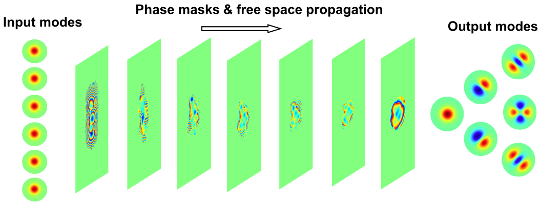
Multi-plane light conversion (MPLC) has recently been developed as a versatile tool for manipulating spatial distributions of the optical field through repeated phase modulations. An MPLC Device consists of a series of phase masks separated by free-space propagation. It can convert one orthogonal set of beams into another orthogonal set through unitary transformation, which is useful for a number of applications. In telecommunication, for example, mode-division multiplexing (MDM) is a promising technology that will enable continued scaling of capacity by employing spatial modes of a single fiber. MPLC has shown great potential in MDM devices with ultra-wide bandwidth, low insertion loss (IL), low mode-dependent loss (MDL), and low crosstalk. The fundamentals of design, simulation, fabrication, and characterization of practical MPLC mode (de)multiplexers will be discussed in this tutorial.
1 Introduction
1.1 MPLC: a historical review
MPLC first emerged as a novel device that can realize unitary manipulation on light’s spatial profile, by using a finite number of phase masks separated by optical Fourier transform or free space propagation [1]. The authors of the very first paper of MPLC soon founded the company Cailabs that focuses on developing the beam-shaping technology. MPLC prototypes that support 3, 6, 10 and 15 modes were soon developed using 7, 7, 14, 20 phase masks, respectively [2, 3, 4, 5, 6]. The phase masks of MPLC can contain millions of pixels in total, which represent a huge parameter space for designers to control the wavefront of an optical beam. Considering the complexity of the MPLC system, Boucher et al. applied the filtered random matrix (FRM) theory to show that, when considering high-dimensional modes outside the subspace of modes that MPLC is designed to shape, it behaves like a random scattering medium with limited number of controlled channels [7].
For a real practical device, usually the input and output only contain a finite set of orthogonal spatial modes, which merely spans a subspace of the total mode space supported by the MPLC. Within the finite set, modes are mutually incoherent. In telecommunication for example, as a mode (de)multiplexer, the inputs are spatially separated Gaussian spots while the outputs are spatially overlapped orthogonal mode sets, e.g. Hermite Gaussian (HG) or Laguerre Gaussian (LG) modes. These modes are more interested because of many good properties they possessed, e.g. HG modes are eigenmodes of the graded-index multimode fiber (GI-MMF) [8], and LG modes is more resistant to atmospheric turbulence [9]. The basic structure of an MPLC that functions as a mode multiplexer is shown in Fig.1.
Different methods have been used to optimize the patterns of phase masks. Since design of MPLC falls in the general category of inverse design, quite often, patterns of the optimized phase masks are not intuitive. Modified wavefront matching is the method commonly used to iteratively update phase masks [10]. Very like the famous Gerchberg–Saxton algorithm, it is not directly guided by any cost function but still converges fast through the gradient descent search. Another common method is to use algorithm differentiation on a cost function [11], for example, the gradient descent based backpropagation of neural networks [12, 13, 14]. Regularization terms can be added to the cost function to smooth the mask, such as the well known total-variation (TV) norm [15]. Note that the multimode converters in [14] uses hundreds of phase planes, which is more like a miniaturized version of the continuous, adiabatic photonic lantern rather than a free space device like MPLC.
Generally transforming modes require an order of phase masks [16]. But there is still no theory guides the minimum number of planes required for a specified transition. Actually, many factors affect the number of phase masks required to achieve a certain performance, such as the number of modes, the geometric layouts of the spots array at input, the mapping order, the chosen output mode sets, the pixel size, the mask plane spacing, etc. In 2017, Fontaine et al. at Bell Labs found a magic mapping relation: From Cartesian points to the Cartesian indices of HG modes, mode conversion can be realized using remarkably few planes of equally spaced phase masks [17]. Since then, 210/325 modes using 7 phase masks [18] and 1035 modes using 14 phase masks [19] have been demonstrated. The reason for reduction of phase masks was explained by the separable mode basis theory in [6].
Although MPLC has many applications beyond the area of optical communication, this tutorial is mainly focus on devices for the telecommunication. The terminology common to all communication devices appear in this tutorial have the same meaning as section II of ref[16]. Within telecommunication, especially within mode-division multiplexing which will be briefly introduced in the next section, mode (de)multiplexers are the most critical device.
The performance of a mode (de)multiplexer is usually characterized by the mode coupling matrix . The crosstalk matrix is given by , where is the conjugate transpose of . By cascading a pair of multiplexer and demultiplexer, matrix is usually obtained by measuring power at all output ports when launching light into each input port. After recovering the amplitude and phase of outputs using methods like the off-axis digital holography [18], the matrix is retrieved by projecting the actual output modes to a set of desired mode basis. Then we apply the singular value decomposition (SVD) [20],
| (1) |
where and are unitary matrices, representing linear supposition of the input/output mode basis with lossless mode coupling. is a diagonal matrix with non-negative real numbers called singular values, representing loss propriety of the device without crosstalk. As a result, the SVD operation projects the modes of the (de)multiplexer to another mode basis that separates crosstalk and loss. A good understanding between the two can be found in the supplementary of [18]. With the singular values, we can define the insertion loss (IL) and mode-dependent loss (MDL) as below
| (2) |
| (3) |
where are the singular values of the complex mode coupling matrix .
In terms of other MPLC-based devices for optical communication, in 2018, an MPLC-based mode scrambler that completely inverts the first 10 modes of a GI-MMF was demonstrated to reduce the computational load of DSP [21]. In 2019, a mode demultiplexing hybrid (MDH) was proposed to simplify the optical front end of mode-division multiplexing (MDM) receivers by combining the functionality of mode demultiplexing and optical 90∘ mixing [22]. In 2021, an MPLC based stokes vector direct detection receiver was reported to measure the spatial complex amplitude and coherence without using a reference beam [23]. The authors also contributed to the design of a mode coupler [24], a reconfigurable mode router [25], and an ultrabroadband optical hybrid [26] using the concept of MPLC. MPLC has also been reported to combat the atmosphere turbulence, either using the static scheme [27, 28] or the dynamic scheme [29].
Based on the space-time duality: diffraction in space is similar to dispersion in time, the concept of MPLC has also been extended to temporal domain for waveform shaping. Mazur et al. used a series of phase modulators separated by dispersive all-pass filters to fulfill a lossless optical arbitrary waveform generator [30]. Ashby et al. proposed a similar scheme for applications in quantum information science, which will be favored by the quantum community because of the lossless operation inherited in unitary transformation on temporal modes [31]. Combined with a wavelength selective switch (WSS), MPLC has also been used to control both the spatial and temporal properties of light at the same time [32, 33]. MPLC is also a versatile tool to study the spatiotemporal properties of light [34, 35].
In 2018, Lin et al. trained the neural networks for all-optical machine learning, which are formed by several transmissive phase masks in a similar structure to MPLC [12]. Since then, the potential of using MPLC to do matrix multiplication at light speed has raised much attention [36, 37, 38], such as the research on photonic Ising machine [39] and the neuromorphic optoelectronic computing [40]. In 2022, Ozer et al. reported using an MPLC-based mode sorter for super-resolution imaging [41].
For small volume or integrated MPLC, besides the millimeter-sized one mentioned above [14], a 3-mode MPLC using the metasurface design was reported in 2020 [42]. Mazur et al. demonstrated 36- and 45-mode MPLCs with a reduced size [43]. Pastor et al. proposed to used arrays of phase shifters and multimode interference (MMI) waveguides to implement arbitrary unitary transformation[44]. Researchers from Yoshiaki Nakano’s group in Japan are developing integrated reconfigurable optical unitary converters (OUCs), and found OUCs based on the MPLC structure is more robust to fabrication errors than the traditional Mach-Zehnder interferometer (MZI)-based OUC [45, 46, 47].
Against from the trend of trying to minimize the structure, the other attempt is designing large-area MPLCs which could be used for high power applications. Cailabs has developed the CANUNDA solution for laser machining by shaping high-power continuous or pulsed beam [48]. At CREOL there is on-going research of using large-area non-mode-selective MPLC [49] for high-power wavefront synthesis, which could be used in applications such as long distance free space communication in the turbulent atmosphere.
1.2 Mode-division multiplexing in optical communication
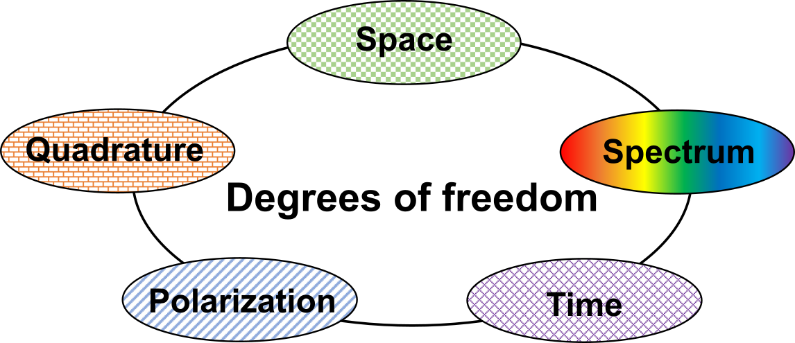
Optical fiber communication, as the backbone infrastructure of internet, has been supporting our increasingly information driven society for many decades. So far much of this progress has been in exploring the data-carrying capacity of a single mode fiber (SMF). To achieve this goal, researchers have attempted to multiplex information into time, frequency, polarization, quadrature (amplitude and phase) of an optical field, as shown in Fig.2. In all these methods, most data traffic demand has been met by the wavelength-division multiplexing (WDM) technology, which increases the spectral bandwidth of fiber-optic communication channel by 2 orders of magnitude in the past two decades. The deployment of broadband, low noise Erbium doped fiber amplifiers (EDFAs) enables amplification of hundreds of wavelength channels simultaneously. Polarization multiplexing has been used to double the transmission capacity. In addition, the reviving coherent optical communication system enables use of advanced modulation formats (e.g., quadrature phase-shift keying (QPSK), quadrature amplitude modulation (16 QAM, 64 QAM, etc.) in the entire amplitude-phase complex plane. With the coherent detection of the complex electrical field, phase and polarization management, dispersion and nonlinear compensation are available by the digital signal processing (DSP) [50]. Actually, the spectral bandwidth of the fiber-optic communication channel can be further increased by exploiting the low-loss transmission window of optical fiber beyond the C bands (5THz, 1530 – 1565 nm) by using the dry fibers [51] or the hollow-core fibers, which promises roughly 10 capability of increase if using the entire O through L bands (50 THz, 1260 – 1625 nm). However, to meet the exponentially growing data traffic, we need to dig out more capacity from the optical fiber. In the information theory, Shannon’s equation gives the maximum capacity that can be reliably communicated over a noisy channel [52, 53]:
| (4) |
where is the signal-to-noise ratio, the factor 2 is the degree of freedom of polarization, B is the system bandwidth, and M is the number of spatial channels. As the capacities provided by the mature technology of WDM and coherent communication quickly approaching their fundamental Shannon limits, the only untapped dimension in single fibers is the spatial dimension. As a ”pre-log” factor in the above equation, it is expected to provide potentially unbounded scaling of capacity [54, 55]. Multi-core fiber (MCF) and multi-mode fiber (MMF) are two most promising fibers supporting space-division multiplexing (SDM). And MCF is usually thought as a transition technology from current SMF to the ultimate goal of MMF, because MMF provides the highest density of spatial channels [56]. As a result, mode-division multiplexing (MDM) comes to the forefront of the optical communication research.
Mode (de)multiplexers are the necessary components to interface the transceivers with the MMF. Of all the mode (de)multiplexing devices, MPLC stands out because it has shown great potential in designing devices with ultrabroadband, low insertion loss (IL), low mode-dependent loss (MDL), low crosstalk, in addition to scaling to large number of modes and large-scale fabrication capability. In 2021, Peta-bit transmission has been demonstrated using a 15-mode MPLC [57]. The record was soon overtaken by a 1.53 Peta-bit/s transmission using 55 modes by the same group in 2022 [58].
2 MPLC-based mode (de)multiplexers
In this section, we explain the fundamentals of design, simulation, fabrication, and characterization of practical MPLC mode (de)multiplexers.
2.1 Simulation
2.1.1 Broadband, reflective MPLC with tilted angles
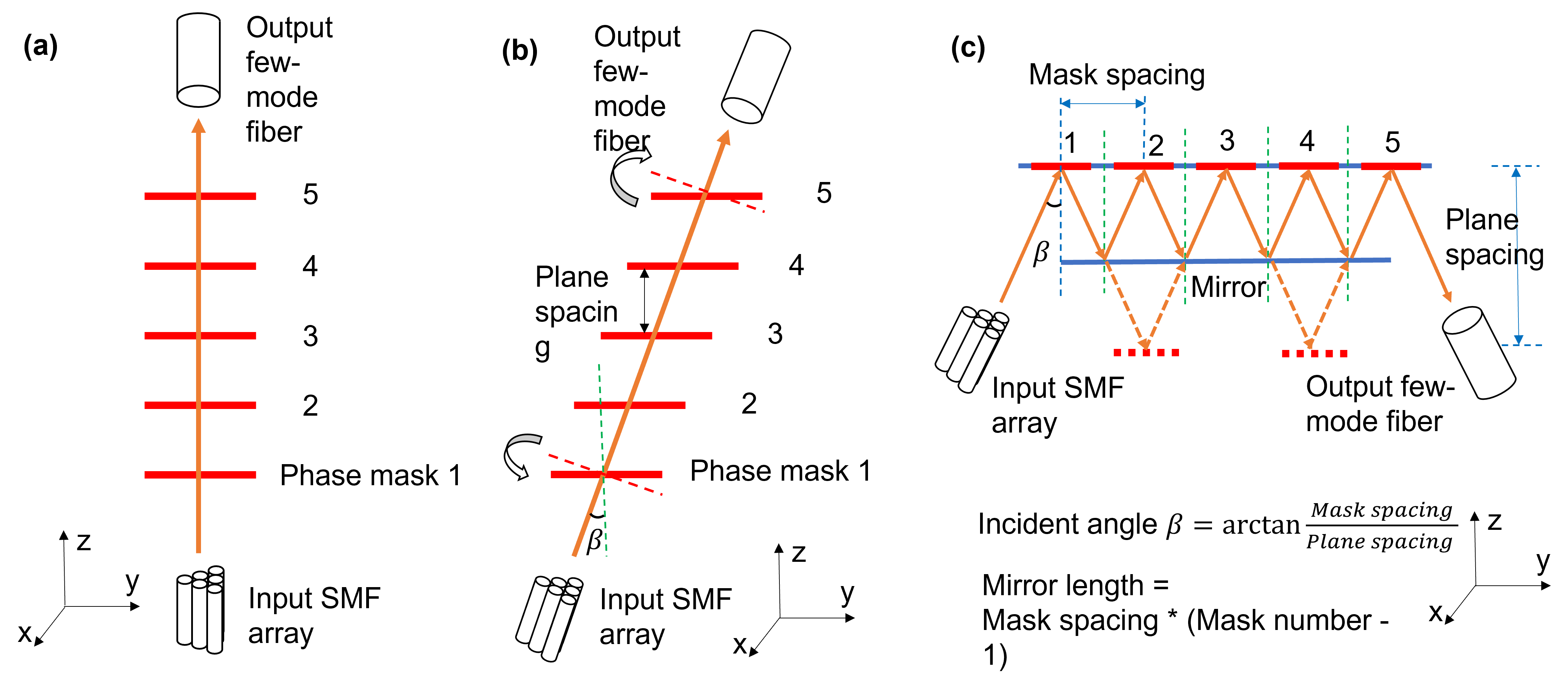
A simple MPLC design starts with the transmissive architecture where the incident beam is normal to the phase masks as shown in Fig.3(a), whereas a practical MPLC usually comes in the form of a folded cavity including a phase mask plane and a mirror plane, as shown in Fig.3(c). The folded cavity simplifies the alignment and assembling of a real MPLC device. In Fig.3(a), traditional angular spectrum method (ASM) is used for free space propagation. However, traditional ASM has a constraint in simulating diffraction: The incident beam must be normal to the input and output plane. i.e., no tilted planes are allowed. It also requires the input sampling window and the output sampling window have the same size and center, which increases the computational load dramatically when the output plane is translated horizontally, as this sampling window has to be increased to be able to contain both the input field as well as the output field. Therefore, traditional ASM limits the ability to simulate a real MPLC device with an incident angle.
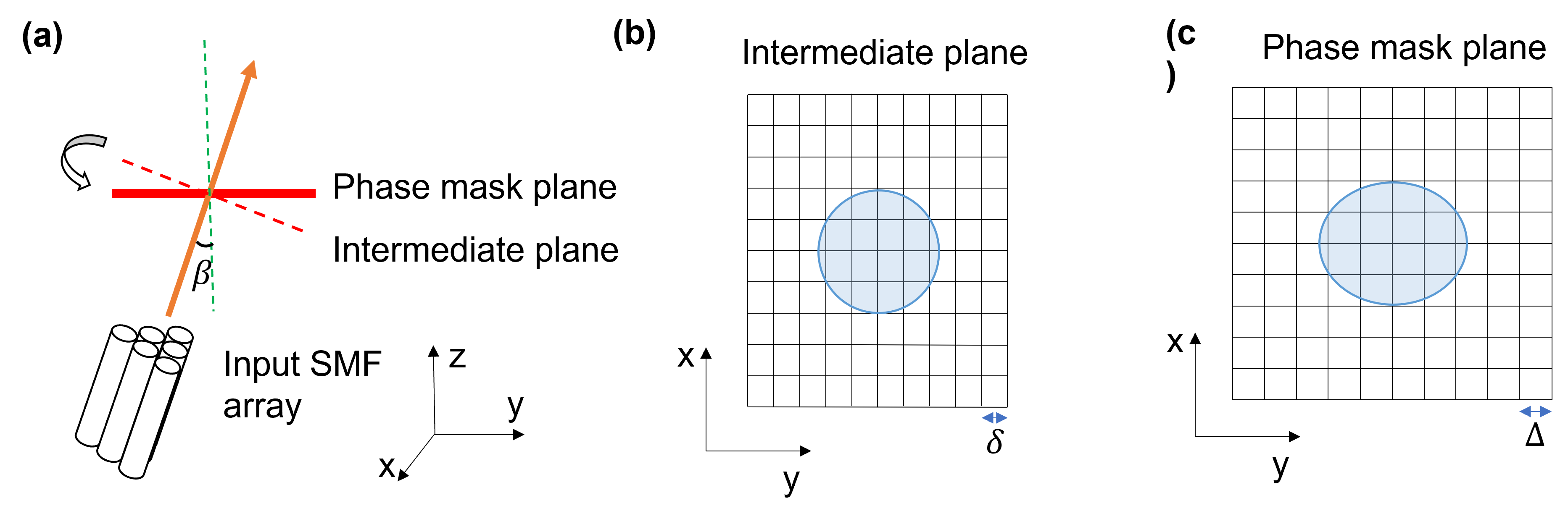
Before explaining the reflective design of Fig.3(c), we use Fig.3(b) as an intermediate step to help understand the process. In Fig.3(b) we build a coordinate system where the incident beam has a tilted angle relative to the direction. The translated ASM [59, 60] is applied to simulate beam propagation between horizontally shifted planes. The translated ASM has a similar numerical complexity as the traditional ASM. It takes the vector phase term in direction out of the Fourier integral as a carrier frequency and let the sampling window shifts together with the phase mask. This helps relieve the sampling requirement in the calculation. However, it should be noted that the collimated beam coming out of the input single-mode fiber array or the beam going into the output few-mode fiber has a wavefront normal to the optical axis. So, a rotation is necessary before multiplying the phase pattern of the first phase mask at the input or after the last phase mask at the output, respectively. One calculation method for optical diffraction on tilted planes is to use the coordinate rotation in Fourier domain [61]. However, this is based on a nonuniform sampling interval in the Fourier plane and requires two-dimensional (2D) interpolation, which has created serious computational complexities. Readers interested in details of this method can refer to chapter 9 of Dr. Matsuhima’ s new book [62]. For small incident angle (less than 10 degree, which is the common case for a MPLC device) however, we can simply rescale the coordinate by , which will be talked in detail in Fig.4. In certain special cases, if we know the analytic equation of the input/output beam (e.g., Gaussian beam, HG modes, LG modes), the field distribution cut by a titled field can be written directly with coordinates rotation. In the configuration of Fig.3(c), the incident angle is determined by the mask spacing and the plane spacing. The mask-spacing is the distance between two adjacent masks on the mask plane, which is usually same as or slightly larger than the mask width in the real design. The mirror width should be diced to the exact length for not blocking the input/output beam, which is the product of the mask-spacing and (mask number-1). The height of the mirror can be oversized to collect more diffracted beam. Note that instead of Fig.3(c), Fig.3(b) is how the computer program understands the physical structure. The shared MATLAB code in [18] gives the basic example code of the structure in Fig. 3(a), which is a good starting point to design reflective MPLCs.
Figure 4 shows the approximation that the field on a tilted plane can be calculated by re-scaling the sampling grid in the direction. The re-scaling factor is given by . After re-scaling, a perfect circle (resembling the Gaussian mode) in the intermediate plane is stretched to an ellipse in the phase mask plane, as shown in Fig.4(b) and (c). We choose to use equidistant sampling grids (square grids) for the phase mask calculation because the fabricated phase masks or phase-only liquid crystal on silicon (LCoS) devices have square pixels. As a result, the sampling grids on the intermediate plane have a rectangular shape.
It’s ideal to consider a broadband design at the beginning to generate very smooth phase masks. This also brings the benefit of improving the tolerance to misalignment. Introducing broadband design can be realized by simply modifying the original code of updating phase masks. The trick is besides taking the average phase differences of the forward and backward field of all spatial modes, we can add another loop to average at several wavelengths close to the center wavelength. Besides the multi-wavelength optimization, ref[17] also provides other suggestions to smooth phase masks. The “equivalent” function of wavelength and mode leads to another design from the author – a wavelength-mode sorter [63], which may find applications in spectral/wavelength beam combining. That design was later experimentally verified by a group at Shenzhen University [64].
2.1.2 Sampling requirements
The transfer function of free space, or the kernel of the angular spectrum method (ASM), is given by [65]
| (5) |
with . After reorganizing the term, we got an ellipsoid function:
| (6) |
The above ellipsoid equation is shown in Fig.5(a).
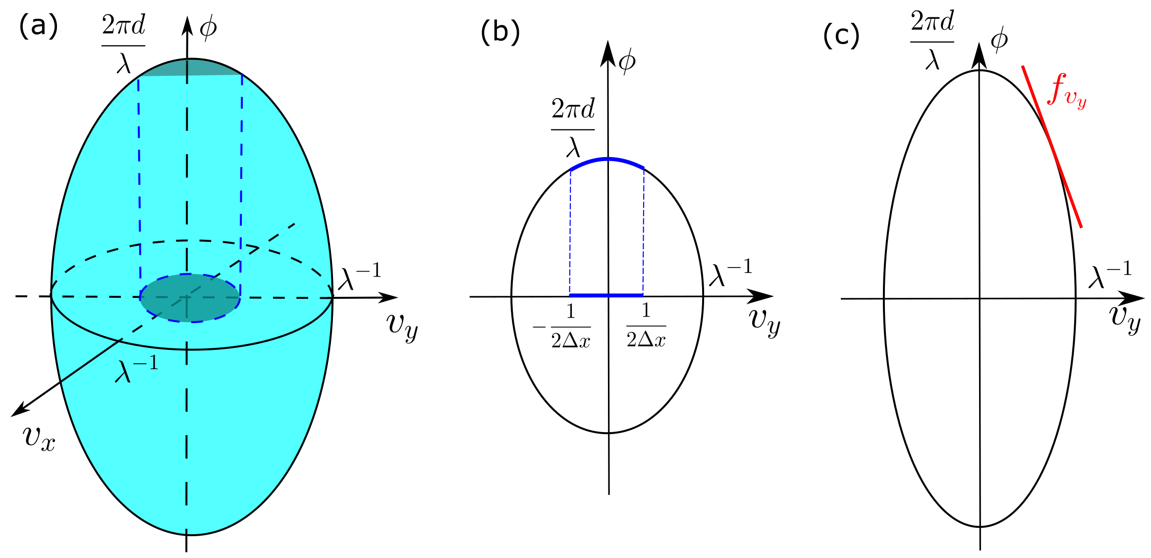
In the digitized version, the sampling points in the spatial domain is
| (7) |
where and are the grid size, or pixel size for the fabricated phase masks or LCoS. Without loss of generality, we assume here. and are the pixel numbers in and direction, respectively. The corresponding sampling points in the Fourier domain (or k-space, with ) is
| (8) |
where and are the grid size in the Fourier domain. The spatial frequency range of is to . The sampling range in k-space is inversely proportional to the pixel size, but not related to the pixel number. To avoid aliasing, sampling points (pixel number) and must be large enough to resolve the finest structures in the optical field.
Note that the foot of the ellipsoid is always fixed at , while the height is related to the propagation distance . As increases, the slope increases dramatically which puts a more strict constraint for the sampling requirements. When is large enough, it will always introduce aliasing without limiting the bandwidth in the ASM method. In Dr. Matsushima’s digital holography book [62], a band-limited ASM method is discussed by adjusting the cutoff frequency as propagation distance changes.
As shown in Fig.5(c), the slope of the ellipsoid gives the ”local spatial frequency”, which is shown below and is proportional to the distance .
| (9) |
Considering for example, the maximum of local spatial frequency is given by
| (10) |
If we take and into above equation, and considering the Nyquist sampling condition (sampling frequency should be at least twice of the highest frequency of the signal), i.e.,
| (11) |
we will get
| (12) |
For MPLC with a pixel size of
For a paraxial beam, . The ratio between these two gives us a sense if we are in the paraxial domain. In order to make sure the paraxial beam condition (also known as Fresnel approximation or parabolic approximation) is satisfied, we expand the phase term by Taylor expansion
| (13) |
For the parabolic approximation to be valid, the third phase term should be much less than , i.e.,
| (14) |
which gives another constraint on if we use and ,
| (15) |
For the MPLC with at 1550 nm, mm.
Note that conditions Eq.(12) and Eq.(15) is sometimes too strict as it requires the entire sampling range to satisfy the Nyquist sampling condition or parabolic approximation while in reality the signal bandwidth is much smaller than the sampling frequency range. The pixel number and can also be very large at the beginning (pad with zeros for the computational window), and the phase mask can be cropped to a smaller size after optimization. In summary, the pixel number and pixel size should be chosen carefully in order to avoid aliasing issues. The pixel size determines the sampled range of the spatial frequency of the angular spectrum method (ASM), and the pixel number determines whether we have enough sampling points to get rid of aliasing.
2.1.3 Considerations for fabrication-ready design
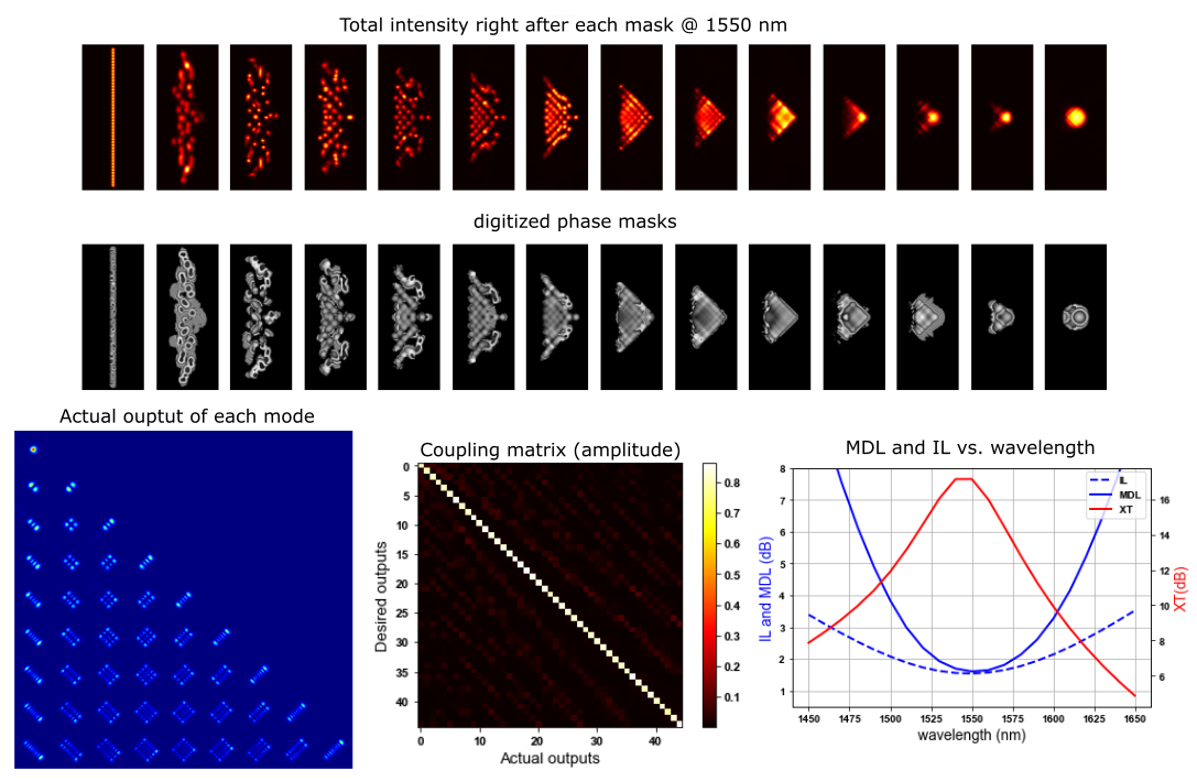
In this section, design of a 45-mode mode selective MPLC with a linear input array was used as an example. Although the specific configuration that inputs arranged in a right triangle shape and outputs using Hermite-Gaussian(HG) modes has been reported as an effective way to reduce the required number of phase masks, using a standard one-dimensional (1D) linear fiber array instead, could potentially reduce the cost of final product and make the alignment much easier.
This MPLC use 14 phase masks to convert a linear input Gaussian spots to HG modes. Input and output beam waist diameter are 70 and 280 , respectively. The beam waist to the first and last mask spacing are 5 mm and 20 mm, respectively. The mask-mirror spacing is 10 mm with an incident angle 7.29 degree. Each mask has a pixel number of 1200 by 512 and a pixel size of 5 .
Because the mapping order from the right triangle to the HG modes is already known to reduce the number of phase masks [18], the mapping order from the linear array to the triangle array should also be optimized to effectively use the first 7 phase masks. Ideally, total deflection angles of all beams should be minimized to encourage smooth phase mask solutions. In my design, I found directly optimizing from a linear array to the HG modes using the wavefront matching method doesn’t give good results. As a result, I optimized the second to the last mask first with input positions of each beam manually set for the first mask, as shown in Fig. 6. For the first mask, the spots layout should span an area as large as possible (which was found helpful to reduce MDL) and has a shape between the linear array and the right triangle array.
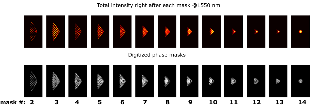
After this procedure, these masks were used as the initial state of the entire optimization. The results are shown below in Fig. 7. Note the pixel number of each mask was also extended to 1800 by 1024 by padding zeros in the optimization to avoid aliasing. After convergence, it was cropped to 1200 by 512 to save space on the wafer.
To fabricate the reflective phase mask using the multi-step binary lithography method, we need to etch multiple steps to give digitized phase levels between 0 and phase shift. For example, digitizing to 64 levels needs 6 steps as . 2 corresponds to 775 nm etch depth at 1550 nm (Recently, MPLC with 8 phase wraps was found to have better performance than their 2 counterparts using less phase masks [66]). After using the function extracting the phase term , by default the phase is wrapped between and and the background is 0. Directly mapping the phase to the etching depth as shown in Fig.13(a) is usually not desired for fabrication, as the factory (SILIOS Technologies, Holo/Or, etc.) don’t want to etch the background. This can be simply solved by a trick,
| (16) |
After the above conversion, the background, originally with a phase 0 (corresponding to an etch depth of 775/2 nm), is shifted to (corresponding to an etch depth of 0).
2.2 Experiment
2.2.1 Make a collimated linear fiber array
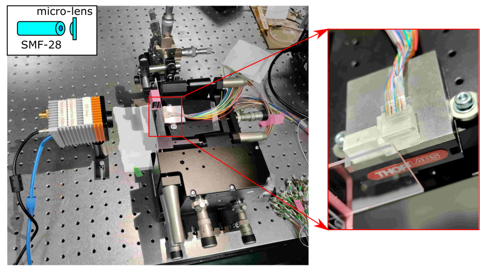
A six-axis stage with sub-micron resolution (Thorlabs, MAX601D/M - 6-Axis NanoMax Stage) was used to assemble the collimated linear fiber array. Usually the fiber array with a standard pitch (127 or 250 ) was used. The microlens array (SUSS MicroOptics) with the same pitch and anti-reflection coating between 1520 nm and 1620 nm was used to collimate the beam. A plano-convex lens is usually used to collimate a beam with the flat surface facing the fiber tip. However, in the experiment shown in Fig.8, the microlens array we are using (pitch = 127 , size 6.658 mm 3.229 mm, radius of curvature 0.155 mm) has a thick fused silica substrate. The focal length is so short that the focal point on the flat surface side is buried inside the substrate, so we have to use the convex surface facing the fiber array. We glue the corner of the flat surface of the microlens array (with a tiny amount of glue) to a glass plate first and then bring it to the V-grove fiber array. After proper alignment all ports should have a perfect Gaussian shape and the beam waist radius was measured to be close to 35 . Then we use UV glue to fix the microlens array to the fiber array and pull the glass plate in backward direction to detach it. A good collimated fiber array has similar collimated beam size for all ports with small pointing errors.
2.2.2 Retro-reflection in alignment
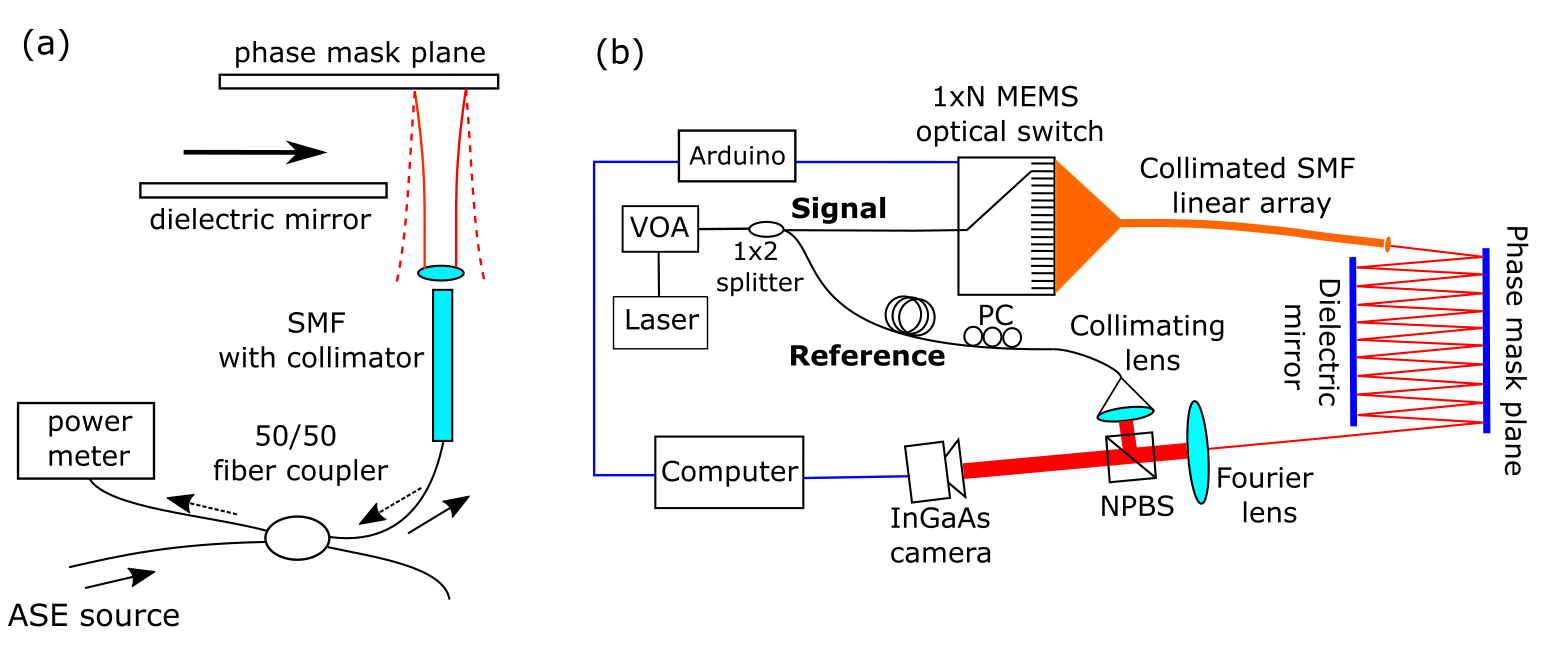
The phase mask plane is glued on a glass base first. The dielectric mirror and input fiber array are held on a 6-axis (x,y,z,pitch, yaw, roll) stage respectively. As shown in Fig.9(a), an ASE source, a 50:50 fiber coupler, a power meter and a collimated SMF are used to assist the alignment. The alignment takes 3 times of retro-reflection. First, the dielectric mirror was moved away and we do retro-reflection on the empty region on the phase mask. We adjust the stage holding the SMF collimator until maximum power reading on the power meter. In this way, we make the beam normal to the phase mask plane. Next the dielectric is moved in and do retro-reflection on the mirror. This time we adjust the 6-axis stage holding the mirror until maximum power reading. After this step we know the mirror is parallel to the mask plane. Finally, we do retro-reflection with the input fiber array to make it normal to the mask plane first. Then we rotate the fiber array to the correct incident angle.
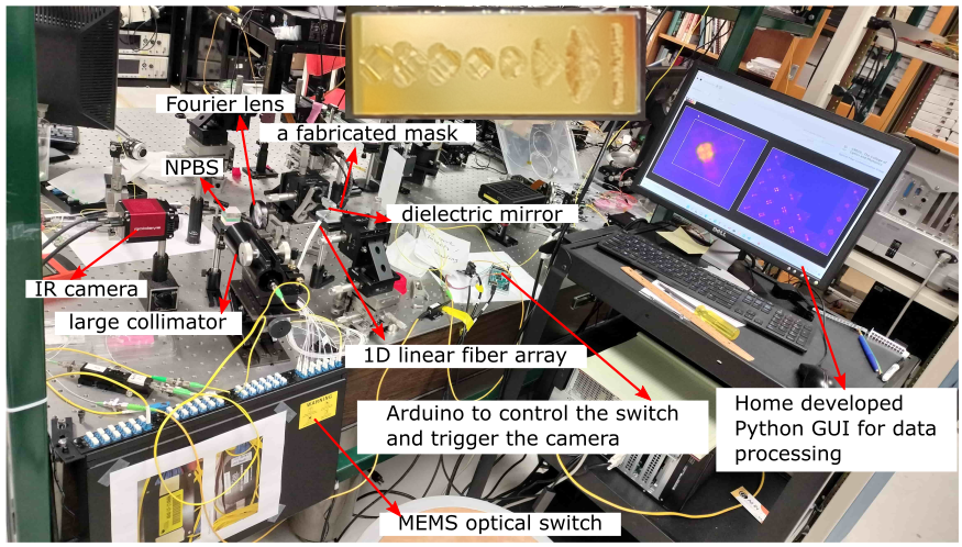
Fig.9(b) shows the experimental setup to characterize the MPLC using off-axis digital holography. The 1N optical switch is used to selectively launch beam to all output HG modes. The optical switch is synchronized with the InGaAs camera so that whenever the input port changes, a frame of raw image is captured. A Fourier lens (2f system) was put at the output of MPLC, and it relays the flat wavefront of the beam waist to the camera sensor plane. A large collimating lens is used for the reference arm to generate quasi-plane beam. After collimating, the beam waist diameter of the reference should be larger than the size of the camera sensor.
2.2.3 Off-axis digital holography
Off-axis digital holography was used to measure the complex field and further the complete mode transfer matrix of the mode multiplexer/demultiplexer. Digital holography allows us to do the alignment of optical fields and modes decomposition in the computer, without introducing possible errors of the characterization setup itself [18, 67, 68].
Fundamentals of off-axis digital holography can be found in Dr. Joel Carpenter’s digHolo library shared on GitHub and YouTube [69]. Chapter 3 of Dr. Heide’s dissertation is another good reference for the basics of off-axis digital holography [70]. Ref[71] talks about some practical considerations when doing off-axis digital holography.
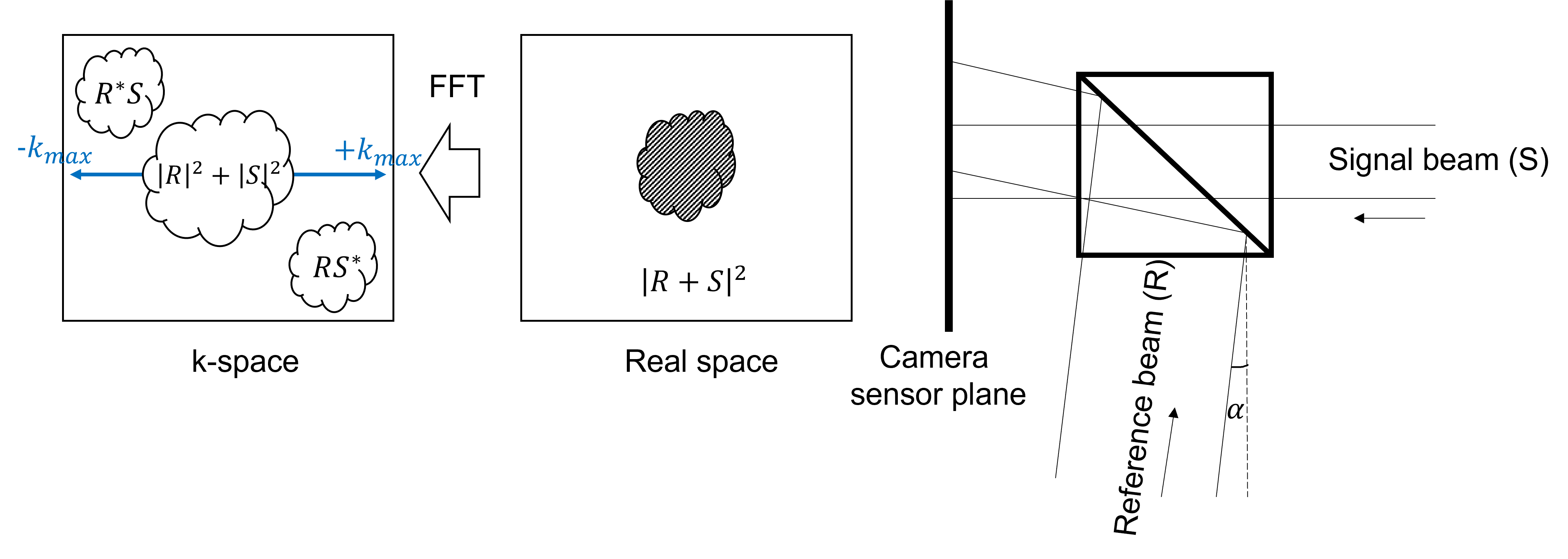
The schematic of off-axis digital holography is shown in Fig.10. The complex field of the signal beam can be extracted from the 1st order in the Fourier domain. Ideally the lengths of the signal arm and reference arm should be matched and a highly coherent laser is used to increase the contrast of the fringes. The signal and reference fields should be mutually coherent during the exposure of the camera so that their relative phase is stable when capturing a frame. The maximum tilt angle of the reference beam is limited by the pixel size of the camera and the wavelength. As we discussed the in chapter 2.1.2, the spatial frequency range is to , so that . For paraxial beam, we have
| (17) |
For 1550 nm and a pixel size of 3030 of the Goldeye camera (Allied Vision, Goldeye G-008 SWIR TEC1), the maximum angle is about 1.48 degree. If the tilt angle is larger than this value, there will be more than one interference fringes inside one camera pixel which causes aliasing, as a result the fringe contrast reduces and the recovered field is not accurate.
In real experiment, misalignment of the Fourier lens, tilt of the camera sensor, or the quasi-plane feature of the big reference beam introduce phase errors to the system. The linear (tip and tilt) and quadratic (defocus) phase errors, and the centering in and of the recovered field, as well as the beam size and rotation angle of the reference modes should be optimized before calculating the mode transfer matrix. Linear phase errors can be compensated by centering the beam in the Fourier domain (-space), while centering in and can be done by removing the linear phase in -space. The defocus can be compensated by multiplying a thin lens function in real space.
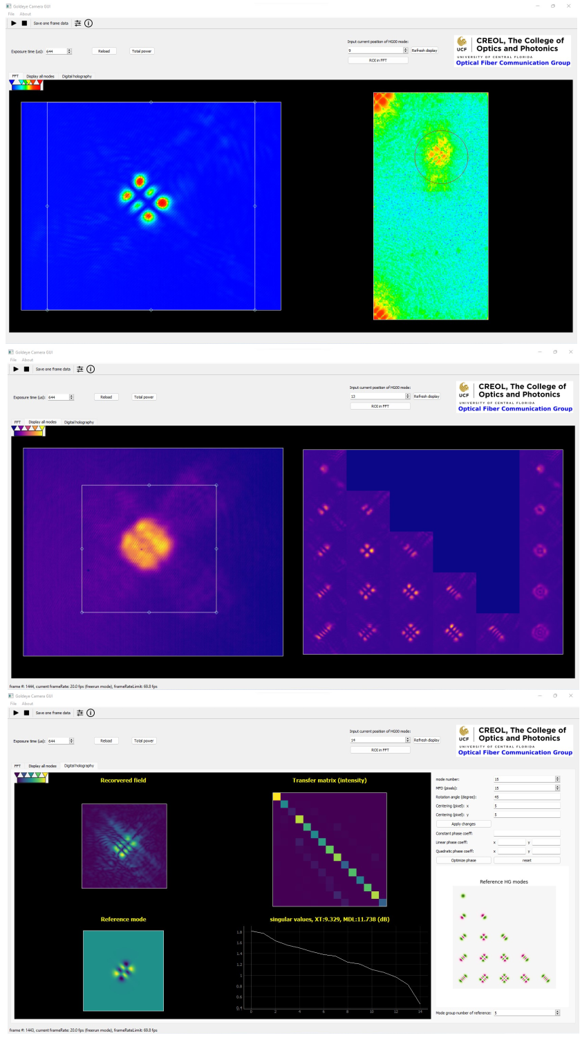
To assist the MPLC alignment and characterization, a graphical user interface (GUI) was developed in the lab as shown in Fig.11. The top figure shows the raw image on the left and the real FFT on the right, with a circle ROI (region of interest) filter. The middle figure shows the summation of all raw images on the left, and all output modes corresponding to each input port on the right. This is enabled by synchronizing the optical switch and the camera using an external trigger. Modes within the same row belong to the same mode group and are degenerate. The last column sums the intensity of all modes of the same group and shows shapes of concentric circles as mentioned in [8]. The bottom figure shows the intensity of the recovered field, the ideal mode to do overlap integral, the mode coupling matrix, and the singular values, XT and MDL values. If the data is processed fast enough, the mode coupling matrix, XT, and MDL values can be updated almost in real time, which is very helpful to align the MPLC. PyQt5 and PyQtGraph [72] packages were used for the GUI geometric layout. Multi-threading programming could be applied to improve the processing speed of the GUI.
2.2.4 Make a multimode collimator
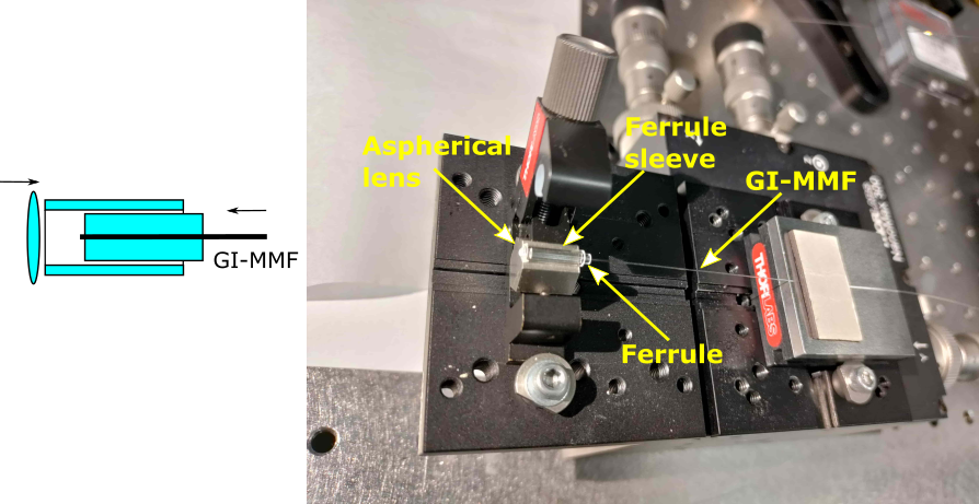
A multimode collimator is necessary if we want to couple the free space output of MPLC into a MMF [73, 16]. Since HG modes are the eigen modes of a medium with parabolic index profile, the GI-MMF is usually used. As shown in Fig.12, first we insert the cleaved MMF into a ferrule and glue it. Then we glue an aspherical lens or a GRIN lens to the ferrule sleeve. Finally, the glued ferrule is carefully inserted into the sleeve and by adjust the spacing to the lens to make sure it’s focused to the far field, i.e., collimated. The designed output beam size of the MPLC determines which lens to use. It’s important to make sure the collimated beam waist is very close to the lens surface so that we can glue the multimode collimator on the same glass base holding the MPLC by matching their beam waists.
2.2.5 Multi-step binary lithography
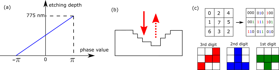
Multi-step binary lithography (also known as gray-scale lithography) is the technique to fabricate phase masks on the fused silica wafer. Fig.13(a) shows the mapping relation between etching depth and the wrapped phase of the mask when the center wavelength is 1550 nm. Fig.13(b) schematically shows the cross-section of the etched wafer with digitized steps. Reflected beam accumulates different phases at different pixels due to the phase retardation encountered at that pixel. Note that for a centering wavelength of 1550 nm, maximum etching depth is 1550/2 = 775 nm because it works in the reflective mode. In Fig.13(c) we illustrate the principle of multi-step binary lithography. Taking for example, 3 etching steps give 8 discrete phase levels between 0 and 7, which are randomly distributed in a 33 box. Next we convert each number to the binary format and number ”1” in a certain digit means it’s going to be etched. Red, blue and green color is used to show the etching profile corresponding to a certain digit respectively. 3 layers of photomasks are required for this fabrication. Each layer has a different etching depth related to the ”weight” of that binary format.
Besides varying the physical thickness to generate gray-scale phase profiles, [74] also mentioned using a photosensitive material together with a digital micromirror device (DMD) to create arbitrary phase profiles. The spatial shape of the phase pattern is controlled by the DMD, and the phase value at each pixel is determined by the exposure time of micromirrors in the ”on” position.
2.2.6 Align a 15-mode MPLC with the LCoS and fabricated phase masks
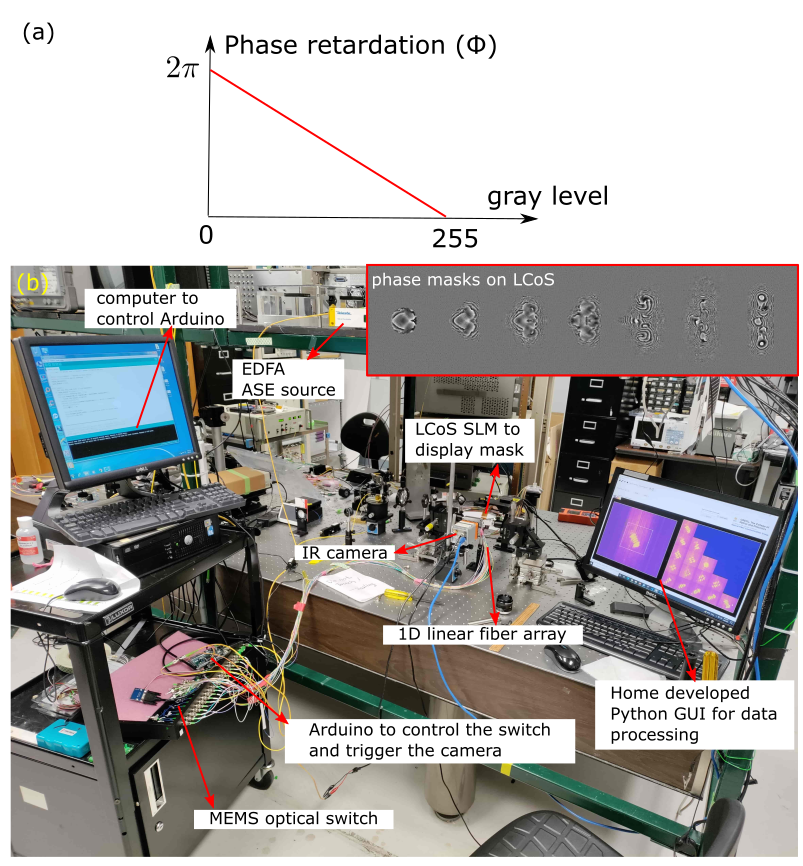
In this section we show the experimental setup for the alignment of a 15-mode MPLC using a LCoS and a fabricated phase mask, shown in Fig.14 and Fig.15, respectively. The Holoeye PLUTO-2-TELCO-059 Phase Only LCoS was used for the experiment. It should be noted that the phase response is wavelength dependent. For certain LCoS (like the one used in our experiment) max retardation is present in off state. After calibration the phase retaration is in a decreasing linear manner when addressing gray level from 0-255, as shown in Fig.14 (a). And you need to reverse the phase mask before putting it on the LCoS. We should also pay attention to the fringing field effect of LCoS [75, 76] that introduces inter-pixel crosstalk and gives a larger MDL. This phase-only LCoS is polarization sensitive and only gives pure phase modulation if the input beam has correct polarization, otherwise there will be phase-amplitude crosstalk [77]. [78] briefly reviewed a method to implement amplitude modulation on a phase-only LCoS.
3 Conclusion
Theoretically, MPLC can be used to realize any unitary conversion using a set of phase masks. However, only certain transforms (right triangle array of spots to Hermite-Gaussian modes) was found that only requires a small number of phase masks. The trade-off between the number of phase masks and the performance (bandwidth, MDL, crosstalk, etc.) is a question that needs serious attention at the beginning of every design. In reality, it’s ideal to reduce the number of phase masks both for easy alignment/fabrication and for reducing the total loss of the system. The lithography-defined phase masks can be fabricated at a large scale with a reasonable cost, but will also introduce scattering loss due to the pixelized structures. In theory the loss can be well below 1 dB, but current MPLC devices has a loss between 3 5 dB due to scattering [16]. In the future, we believe new fabrication techniques will bring the experimental loss down to theoretical level and MPLC-based devices will be widely deployed.
References
- [1] J.-F. Morizur, L. Nicholls, P. Jian, S. Armstrong, N. Treps, B. Hage, M. Hsu, W. Bowen, J. Janousek, and H.-A. Bachor, “Programmable unitary spatial mode manipulation,” JOSA A, vol. 27, no. 11, pp. 2524–2531, 2010.
- [2] G. Labroille, B. Denolle, P. Jian, P. Genevaux, N. Treps, and J.-F. Morizur, “Efficient and mode selective spatial mode multiplexer based on multi-plane light conversion,” Optics express, vol. 22, no. 13, pp. 15599–15607, 2014.
- [3] P. Genevaux, C. Simonneau, G. Labroille, B. Denolle, O. Pinel, P. Jian, J.-F. Morizur, and G. Charlet, “6-mode spatial multiplexer with low loss and high selectivity for transmission over few mode fiber,” in 2015 Optical Fiber Communications Conference and Exhibition (OFC), pp. 1–3, IEEE, 2015.
- [4] G. Labroille, P. Jian, N. Barré, B. Denolle, and J.-F. Morizur, “Mode selective 10-mode multiplexer based on multi-plane light conversion,” in Optical Fiber Communication Conference, pp. Th3E–5, Optical Society of America, 2016.
- [5] N. Barré, B. Denolle, P. Jian, J.-F. Morizur, and G. Labroille, “Broadband, mode-selective 15-mode multiplexer based on multi-plane light conversion,” in Optical Fiber Communication Conference, pp. Th2A–7, Optical Society of America, 2017.
- [6] S. Bade, B. Denolle, G. Trunet, N. Riguet, P. Jian, O. Pinel, and G. Labroille, “Fabrication and characterization of a mode-selective 45-mode spatial multiplexer based on multi-plane light conversion,” in Optical Fiber Communication Conference, pp. Th4B–3, Optica Publishing Group, 2018.
- [7] P. Boucher, A. Goetschy, G. Sorelli, M. Walschaers, and N. Treps, “Full characterization of the transmission properties of a multi-plane light converter,” Physical Review Research, vol. 3, no. 2, p. 023226, 2021.
- [8] N. K. Fontaine, R. Ryf, H. Chen, S. Wittek, J. Li, J. Alvarado, J. A. Lopez, M. Cappuzzo, R. Kopf, A. Tate, et al., “Packaged 45-mode multiplexers for a graded index fiber,” in 2018 European Conference on Optical Communication (ECOC), pp. 1–3, IEEE, 2018.
- [9] A. Belmonte and J. M. Kahn, “Optimal modes for spatially multiplexed free-space communication in atmospheric turbulence,” Optics Express, vol. 29, no. 26, pp. 43556–43566, 2021.
- [10] Y. Sakamaki, T. Saida, T. Hashimoto, and H. Takahashi, “New optical waveguide design based on wavefront matching method,” Journal of lightwave technology, vol. 25, no. 11, pp. 3511–3518, 2007.
- [11] A. S. Jurling and J. R. Fienup, “Applications of algorithmic differentiation to phase retrieval algorithms,” JOSA A, vol. 31, no. 7, pp. 1348–1359, 2014.
- [12] X. Lin, Y. Rivenson, N. T. Yardimci, M. Veli, Y. Luo, M. Jarrahi, and A. Ozcan, “All-optical machine learning using diffractive deep neural networks,” Science, vol. 361, no. 6406, pp. 1004–1008, 2018.
- [13] Z. Zhu, J. H. Doerr, G. Li, and S. Pang, “Multiplane light conversion design with physical neural network,” in Digital Holography and Three-Dimensional Imaging, pp. M6A–2, Optica Publishing Group, 2022.
- [14] N. Barré and A. Jesacher, “Inverse design of gradient-index volume multimode converters,” Optics Express, vol. 30, no. 7, pp. 10573–10587, 2022.
- [15] A. Beck and M. Teboulle, “Fast gradient-based algorithms for constrained total variation image denoising and deblurring problems,” IEEE transactions on image processing, vol. 18, no. 11, pp. 2419–2434, 2009.
- [16] N. K. Fontaine, J. Carpenter, S. Gross, S. Leon-Saval, Y. Jung, D. J. Richardson, and R. Amezcua-Correa, “Photonic lanterns, 3-d waveguides, multiplane light conversion, and other components that enable space-division multiplexing,” Proceedings of the IEEE, 2022.
- [17] N. K. Fontaine, R. Ryf, H. Chen, D. Neilson, and J. Carpenter, “Design of high order mode-multiplexers using multiplane light conversion,” in 2017 European Conference on Optical Communication (ECOC), pp. 1–3, IEEE, 2017.
- [18] N. K. Fontaine, R. Ryf, H. Chen, D. T. Neilson, K. Kim, and J. Carpenter, “Laguerre-gaussian mode sorter,” Nature communications, vol. 10, no. 1, pp. 1–7, 2019.
- [19] N. K. Fontaine, H. Chen, M. Mazur, L. Dallachiesa, K. Kim, R. Ryf, D. Neilson, and J. Carpenter, “Hermite-gaussian mode multiplexer supporting 1035 modes,” in Optical Fiber Communication Conference, pp. M3D–4, Optical Society of America, 2021.
- [20] D. A. Miller, “Waves, modes, communications, and optics: a tutorial,” Advances in Optics and Photonics, vol. 11, no. 3, pp. 679–825, 2019.
- [21] J. Li, N. K. Fontaine, H. Chen, R. Ryf, M. Cappuzzo, R. Kopf, A. Tate, H. Safar, C. Bolle, D. T. Neilson, et al., “Design and demonstration of mode scrambler supporting 10 modes using multiplane light conversion,” in 2018 European Conference on Optical Communication (ECOC), pp. 1–3, IEEE, 2018.
- [22] H. Wen, H. Liu, Y. Zhang, P. Zhang, and G. Li, “Mode demultiplexing hybrids for mode-division multiplexing coherent receivers,” Photonics Research, vol. 7, no. 8, pp. 917–925, 2019.
- [23] D. S. Dahl, M. Plöschner, N. K. Fontaine, and J. Carpenter, “High-dimensional stokes-space spatial beam analyzer,” in Frontiers in Optics, pp. FTu6C–2, Optical Society of America, 2021.
- [24] Y. Zhang, H. Wen, S. Fan, H. Liu, R. Sampson, N. Wang, S. Pang, P. LiKamWa, and G. Li, “Slab waveguide-to-fiber coupling based on multiplane light conversion,” in Frontiers in Optics, pp. FW1B–3, Optical Society of America, 2019.
- [25] Y. Zhang, H. Wen, N. K. Fontaine, H. Chen, P. L. LiKamWa, and G. Li, “A reconfigurable broadband space-mode router using multiplane light conversion,” in 2020 IEEE Photonics Conference (IPC), pp. 1–2, IEEE, 2020.
- [26] Y. Zhang, N. K. Fontaine, H. Chen, R. Ryf, D. T. Neilson, J. Carpenter, and G. Li, “An ultra-broadband polarization-insensitive optical hybrid using multiplane light conversion,” Journal of Lightwave Technology, vol. 38, no. 22, pp. 6286–6291, 2020.
- [27] N. K. Fontaine, R. Ryf, Y. Zhang, J. C. Alvarado-Zacarias, S. van der Heide, M. Mazur, H. Huang, H. Chen, R. Amezcua-Correa, G. Li, et al., “Digital turbulence compensation of free space optical link with multimode optical amplifier,” in 45th European Conference on Optical Communication (ECOC 2019), pp. 1–4, IET, 2019.
- [28] A. Billaud, A. Reeves, A. Orieux, H. Friew, F. Gomez, S. Bernard, T. Michel, D. Allioux, J. Poliak, R. M. Calvo, et al., “Turbulence mitigation via multi-plane light conversion and coherent optical combination on a 200 m and a 10 km link,” in 2022 IEEE International Conference on Space Optical Systems and Applications (ICSOS), pp. 85–92, IEEE, 2022.
- [29] R. Alsaigh, N. Fontaine, and M. P. Lavery, “Bulk optical turbulence mitigation using dynamic multiple plane light conversion,” in Complex Light and Optical Forces XVII, p. PC124360H, SPIE, 2023.
- [30] M. Mazur, N. K. Fontaine, H. Chen, R. Ryf, D. T. Neilson, G. Raybon, A. Adamiecki, S. Corteselli, and J. Schröder, “Multi-wavelength arbitrary waveform generation through spectro-temporal unitary transformations,” arXiv preprint arXiv:1907.02595, 2019.
- [31] J. Ashby, V. Thiel, M. Allgaier, P. d’Ornellas, A. O. Davis, and B. J. Smith, “Temporal mode transformations by sequential time and frequency phase modulation for applications in quantum information science,” Optics Express, vol. 28, no. 25, pp. 38376–38389, 2020.
- [32] M. Mounaix, N. K. Fontaine, D. T. Neilson, R. Ryf, H. Chen, J. C. Alvarado-Zacarias, and J. Carpenter, “Time reversed optical waves by arbitrary vector spatiotemporal field generation,” Nature communications, vol. 11, no. 1, pp. 1–7, 2020.
- [33] M. Mazur, N. K. Fontaine, Y. Zhang, H. Chen, K. Kim, R. Veronese, G. Li, L. Palmieri, M. Bigot, P. Sillard, et al., “Gain and temporal equalizer for multi-mode systems,” in Optical Fiber Communication Conference, pp. Th4B–6, Optica Publishing Group, 2020.
- [34] D. Cruz-Delgado, S. Yerolatsitis, N. K. Fontaine, D. N. Christodoulides, R. Amezcua-Correa, and M. A. Bandres, “Synthesis of ultrafast wavepackets with tailored spatiotemporal properties,” Nature Photonics, vol. 16, no. 10, pp. 686–691, 2022.
- [35] Y. Shen, Q. Zhan, L. G. Wright, D. N. Christodoulides, F. W. Wise, A. E. Willner, Z. Zhao, K.-h. Zou, C.-T. Liao, C. Hernández-García, et al., “Roadmap on spatiotemporal light fields,” arXiv preprint arXiv:2210.11273, 2022.
- [36] H. Zhou, J. Dong, J. Cheng, W. Dong, C. Huang, Y. Shen, Q. Zhang, M. Gu, C. Qian, H. Chen, et al., “Photonic matrix multiplication lights up photonic accelerator and beyond,” Light: Science & Applications, vol. 11, no. 1, pp. 1–21, 2022.
- [37] J. Li, D. Mengu, Y. Luo, Y. Rivenson, and A. Ozcan, “Class-specific differential detection in diffractive optical neural networks improves inference accuracy,” Advanced Photonics, vol. 1, no. 4, p. 046001, 2019.
- [38] L. Bernstein, A. Sludds, R. Hamerly, V. Sze, J. Emer, and D. Englund, “Freely scalable and reconfigurable optical hardware for deep learning,” Scientific reports, vol. 11, no. 1, pp. 1–12, 2021.
- [39] D. Pierangeli, G. Marcucci, and C. Conti, “Large-scale photonic ising machine by spatial light modulation,” Physical review letters, vol. 122, no. 21, p. 213902, 2019.
- [40] T. Zhou, X. Lin, J. Wu, Y. Chen, H. Xie, Y. Li, J. Fan, H. Wu, L. Fang, and Q. Dai, “Large-scale neuromorphic optoelectronic computing with a reconfigurable diffractive processing unit,” Nature Photonics, vol. 15, no. 5, pp. 367–373, 2021.
- [41] I. Ozer, M. R. Grace, and S. Guha, “Reconfigurable spatial-mode sorter for super-resolution imaging,” in 2022 Conference on Lasers and Electro-Optics (CLEO), pp. 1–2, IEEE, 2022.
- [42] J. Oh, W. T. Chen, K. Li, J. Yang, M.-J. Li, P. Dainese, and F. Capasso, “Compact mode-division multiplexing with folded metasurfaces,” in Metamaterials, Metadevices, and Metasystems 2020, vol. 11460, p. 114602N, SPIE, 2020.
- [43] M. Mazur, N. K. Fontaine, R. Ryf, H. Chen, D. T. Neilson, and J. Carpenter, “Reduced footprint multiplane light propagation mode multiplexers,” in 45th European Conference on Optical Communication (ECOC 2019), pp. 1–4, IET, 2019.
- [44] V. L. Pastor, J. Lundeen, and F. Marquardt, “Arbitrary optical wave evolution with fourier transforms and phase masks,” Optics Express, vol. 29, no. 23, pp. 38441–38450, 2021.
- [45] R. Tang, T. Tanemura, and Y. Nakano, “Integrated reconfigurable unitary optical mode converter using mmi couplers,” IEEE Photonics Technology Letters, vol. 29, no. 12, pp. 971–974, 2017.
- [46] R. Tang, T. Tanemura, S. Ghosh, K. Suzuki, K. Tanizawa, K. Ikeda, H. Kawashima, and Y. Nakano, “Reconfigurable all-optical on-chip mimo three-mode demultiplexing based on multi-plane light conversion,” Optics Letters, vol. 43, no. 8, pp. 1798–1801, 2018.
- [47] R. Tanomura, R. Tang, T. Umezaki, G. Soma, T. Tanemura, and Y. Nakano, “Scalable and robust photonic integrated unitary converter based on multiplane light conversion,” Physical Review Applied, vol. 17, no. 2, p. 024071, 2022.
- [48] M. Meunier, D. Lemaitre, A. Billaud, A. Queffelec, R. Cornee, G. Pallier, O. Pinel, E. Laurensot, and G. Labroille, “Fully reflective annular laser beam shaping for 1.03 m ultra-high throughput laser beam welding (conference presentation),” in High-Power Laser Materials Processing: Applications, Diagnostics, and Systems IX, vol. 11273, p. 112730H, SPIE, 2020.
- [49] H. Wen, Y. Zhang, R. Sampson, N. K. Fontaine, N. Wang, S. Fan, and G. Li, “Scalable non-mode selective hermite–gaussian mode multiplexer based on multi-plane light conversion,” Photonics Research, vol. 9, no. 2, pp. 88–97, 2021.
- [50] G. Li, “Recent advances in coherent optical communication,” Advances in optics and photonics, vol. 1, no. 2, pp. 279–307, 2009.
- [51] R.-J. Essiambre, G. Kramer, P. J. Winzer, G. J. Foschini, and B. Goebel, “Capacity limits of optical fiber networks,” Journal of Lightwave Technology, vol. 28, no. 4, pp. 662–701, 2010.
- [52] C. E. Shannon, “A mathematical theory of communication,” The Bell system technical journal, vol. 27, no. 3, pp. 379–423, 1948.
- [53] P. J. Winzer, D. T. Neilson, and A. R. Chraplyvy, “Fiber-optic transmission and networking: the previous 20 and the next 20 years,” Optics express, vol. 26, no. 18, pp. 24190–24239, 2018.
- [54] G. Li, N. Bai, N. Zhao, and C. Xia, “Space-division multiplexing: the next frontier in optical communication,” Advances in Optics and Photonics, vol. 6, no. 4, pp. 413–487, 2014.
- [55] D. J. Richardson, J. M. Fini, and L. E. Nelson, “Space-division multiplexing in optical fibres,” Nature photonics, vol. 7, no. 5, pp. 354–362, 2013.
- [56] R. Ryf, M. Fontaine, X. Zhou, and C. Xie, “Space-division multiplexing and mimo processing,” in Enabling technologies for high spectral-efficiency coherent optical communication networks, Wiley Online Library, 2016.
- [57] G. Rademacher, B. J. Puttnam, R. S. Luís, T. A. Eriksson, N. K. Fontaine, M. Mazur, H. Chen, R. Ryf, D. T. Neilson, P. Sillard, et al., “Peta-bit-per-second optical communications system using a standard cladding diameter 15-mode fiber,” Nature Communications, vol. 12, no. 1, pp. 1–7, 2021.
- [58] G. Rademacher, R. S. Luís, B. J. Puttnam, N. K. Fontaine, M. Mazur, H. Chen, R. Ryf, D. T. Neilson, D. Dahl, J. Carpenter, et al., “1.53 peta-bit/s c-band transmission in a 55-mode fiber,” in 2022 European Conference on Optical Communication (ECOC), pp. 1–4, IEEE, 2022.
- [59] H.-h. Son and K. Oh, “Light propagation analysis using a translated plane angular spectrum method with the oblique plane wave incidence,” JOSA A, vol. 32, no. 5, pp. 949–954, 2015.
- [60] A. Ritter, “Modified shifted angular spectrum method for numerical propagation at reduced spatial sampling rates,” Optics express, vol. 22, no. 21, pp. 26265–26276, 2014.
- [61] K. Matsushima, H. Schimmel, and F. Wyrowski, “Fast calculation method for optical diffraction on tilted planes by use of the angular spectrum of plane waves,” JOSA A, vol. 20, no. 9, pp. 1755–1762, 2003.
- [62] K. Matsushima, Introduction to Computer Holography: Creating Computer-Generated Holograms as the Ultimate 3D Image. Springer Nature, 2020.
- [63] Y. Zhang, H. Wen, A. Fardoost, S. Fan, N. K. Fontaine, H. Chen, P. L. Likamwa, and G. Li, “Simultaneous sorting of wavelengths and spatial modes using multi-plane light conversion,” arXiv preprint arXiv:2010.04859, 2020.
- [64] A. Kong, T. Lei, and X. Yuan, “Mode and wavelength hybrid multiplexer enabled by multi-plane light conversion,” in Asia Communications and Photonics Conference, pp. T4A–207, Optica Publishing Group, 2021.
- [65] B. E. Saleh and M. C. Teich, Fundamentals of photonics. john Wiley & sons, 2019.
- [66] N. K. Fontaine, M. Mazur, R. Ryf, L. Dallachiesa, H. Chen, D. Neilson, C. Bolle, and J. Carpenter, “Broadband 15-mode multiplexers based on multi-plane light conversion with 8 planes in unwrapped phase space,” in 2022 European Conference on Optical Communications (ECOC), pp. 1–4, IEEE, 2022.
- [67] N. T. Shaked, V. Micó, M. Trusiak, A. Kuś, and S. K. Mirsky, “Off-axis digital holographic multiplexing for rapid wavefront acquisition and processing,” Advances in Optics and Photonics, vol. 12, no. 3, pp. 556–611, 2020.
- [68] M. Mazur, N. K. Fontaine, R. Ryf, H. Chen, D. T. Neilson, M. Bigot-Astruc, F. Achten, P. Sillard, A. Amezcua-Correa, J. Schröder, et al., “Characterization of long multi-mode fiber links using digital holography,” in Optical Fiber Communication Conference, pp. W4C–5, Optical Society of America, 2019.
- [69] J. Carpenter, “digholo: High-speed library for off-axis digital holography and hermite-gaussian decomposition,” in Digital Holography and Three-Dimensional Imaging, pp. W5A–53, Optica Publishing Group, 2022.
- [70] S. P. van der Heide, “Space-division multiplexed optical transmission enabled by advanced digital signal processing,” 2022.
- [71] N. Verrier and M. Atlan, “Off-axis digital hologram reconstruction: some practical considerations,” Applied optics, vol. 50, no. 34, pp. H136–H146, 2011.
- [72] PyQtGraph, “Pyqtgraph, scientific graphics and gui library for python.”
- [73] Y. Jung, H. Kim, Y. Chen, T. D. Bradley, I. A. Davidson, J. R. Hayes, G. Jasion, H. Sakr, S. Rikimi, F. Poletti, et al., “Compact micro-optic based components for hollow core fibers,” Optics Express, vol. 28, no. 2, pp. 1518–1525, 2020.
- [74] I. Divliansky, F. Kompan, E. Hale, M. Segall, A. Schülzgen, and L. B. Glebov, “Wavefront shaping optical elements recorded in photo-thermo-refractive glass,” Applied Optics, vol. 58, no. 13, pp. D61–D67, 2019.
- [75] M. Persson, D. Engström, and M. Goksör, “Reducing the effect of pixel crosstalk in phase only spatial light modulators,” Optics express, vol. 20, no. 20, pp. 22334–22343, 2012.
- [76] S. Moser, M. Ritsch-Marte, and G. Thalhammer, “Model-based compensation of pixel crosstalk in liquid crystal spatial light modulators,” Optics express, vol. 27, no. 18, pp. 25046–25063, 2019.
- [77] Z. Zhang, Z. You, and D. Chu, “Fundamentals of phase-only liquid crystal on silicon (lcos) devices,” Light: Science & Applications, vol. 3, no. 10, pp. e213–e213, 2014.
- [78] S. Ngcobo, I. Litvin, L. Burger, and A. Forbes, “A digital laser for on-demand laser modes,” Nature communications, vol. 4, no. 1, pp. 1–6, 2013.