figurec
Multi-Robot Path Planning in Complex Environments via Graph Embedding
Abstract
We propose an approach to solve multi-agent path planning (MPP) problems for complex environments. Our method first designs a special pebble graph with a set of feasibility constraints, under which MPP problems have feasibility guarantee. We further propose an algorithm to greedily improve the optimality of planned MPP solutions via parallel pebble motions. As a second step, we develop a mesh optimization algorithm to embed our pebble graph into arbitrarily complex environments. We show that the feasibility constraints of a pebble graph can be converted into differentiable geometric constraints, such that our mesh optimizer can satisfy these constraints via constrained numerical optimization. We have evaluated the effectiveness and efficiency of our method using a set of environments with complex geometries, on which our method achieves an average of free-space coverage and robot density within hours of computation on a desktop machine.
I Introduction
MPP is a unified theoretical model of various applications, including warehouse arrangement [1], coverage planning for flooring vacuuming [2, 3], and inspection planning for search and rescue [4]. Some applications, such as flooring vacuuming, search and rescue, require MPP planners to tackle complex environments. Intuitively, a task can be accomplished more efficiently when more robots are available. However, coordinating a large number of robots for complex environments can incur a high computational cost. Indeed, determining the feasibility of simplified MPP instances have been shown to be PSPACE-hard [5] (for rectangular objects) and strongly NP-hard [6] (for polygonal environments). It is thus unsurprising that brute-force search algorithms [7, 8, 9, 10] are only practical for tens of robots.
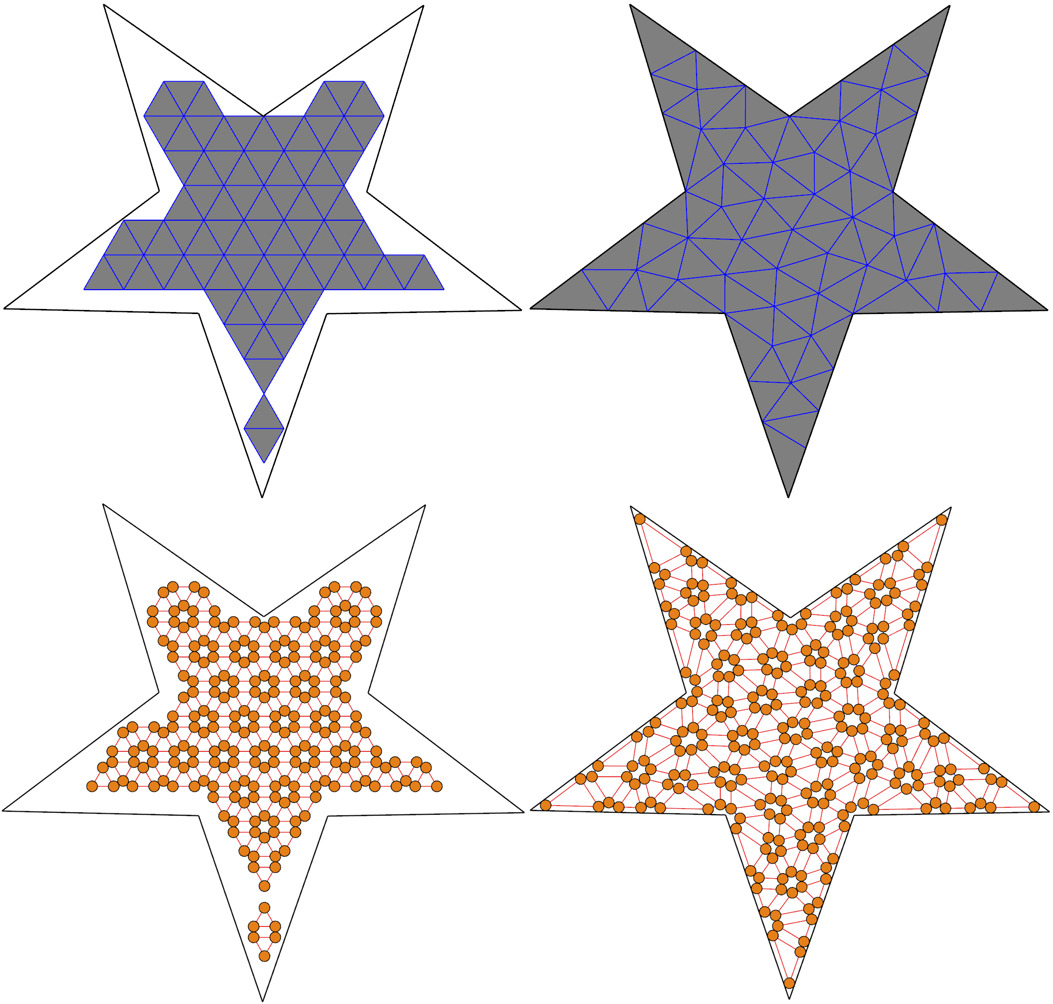
Instead of aiming at generally complex environments, a row of prior works [11, 12, 13] assume that robots can only move on a discrete graph, i.e. robots reside in a discrete set of vertices and move along a discrete set of paths connecting the vertices. For special graphs, such as trees [11, 13] and regular grids [14, 15], determining feasibility and even finding near optimal solutions are polynomial-time solvable. In his recent work, [15] [15] proposed to use curved grids to tile complex environments, but no practical algorithm has been proposed to construct such grids for general geometries. When the shape of an environment has inherent irregularity as illustrated in Figure 1, regular geometric patterns can generate a low-level of coverage or miss curved-boundary regions.
Main Results: We propose a MPP planner that generalizes the idea of graph-based algorithms [1, 16, 15, 12] to complex environments with curved boundaries. Our method uses a special graph topology, on which robots can both move along edges and spin in loops. When the graph satisfy certain geometric properties, it has been shown in [17, 13] that MPP instances are always feasible under certain geometric conditions. We further propose a space-time search algorithm to find parallel motions and greedily improve the makespan. As our key contribution, we show that our graph can be topologically identified with a planar triangle mesh, where the geometric properties of the graph are mapped to differentiable geometric constraints of the triangles. As a result, we can adapt the greedy triangle mesh optimization framework proposed in [18, 19] to optimize a graph that can be embedded into arbitrarily complex environments. During the mesh optimization, a constrained numerical optimization is used to ensure all the geometric constraints are satisfied, i.e., MPP instances are feasible on the graph.
We have evaluated our method on a set of complex environments including 2D floorplans of houses, malls, and maps. Our algorithm is efficient, allowing a graph containing thousands of robots to be generated within an hour on average using a desktop machine. Our generated graph embedding not only aligns well with the curved input boundary but also has high free-space coverage ratio of and robot density ratio of on average. In addition, compared to sequential scheduling, our space-time search algorithm empirically reduces the makespan by a factor of .
II Related Work
In this section, we review related works on MPP, mesh optimization, and graph embedding.
MPP problems in a general setting is intractable [5, 6] and practical methods target at solving restricted problem subclass. If the number of robots is small, then brute-force search is tractable. Early works [8, 20] use RRT or PRM as sub-problem solvers and are thus probabilistically complete. When robots are restricted to move on a graph, their motions can be enumerated using conflict-based search [10] or integer programming [16]. These algorithms are deterministically complete and optimal. For larger robot swarms, state-of-the-art results restrict robots to a graph of special topology such as trees [11] and loops [13], where feasible solutions can be found in polynomial time, and regular grids [15], where near optimal solutions can be found up to a constant factor. Our method resembles [13] in that we allow robots to move and spin. To adapt our method to arbitrarily complex geometries, we cannot guarantee optimality, but we greedily improve optimality via space-time search.
Mesh Optimization algorithm was originally proposed in [19]. The algorithm defines a set of possible remeshing operators that change both the geometry and topology of a mesh and exhaustively applies these operators to monotonically improve a given quality metric. Mesh optimization finds applications in geometric processing [18, 21], and physics-based modeling [22, 23]. These applications use similar algorithm frameworks but differ in the set of operators and the quality metric. Although the framework proposed in [19] is greedy and only achieves local optimality, it is capable of exploring a large portion of solution space. In robotic research, there are similar ideas of cell decomposition [24, 25] and resolution-complete motion planning. Meshes are also used in distributed multi-robot coordination [26, 27] that considers moving a group of robots while maintaining given topological patterns.
Graph Embedding applies the discrete graph theory of MPP to continuous environments. It has been used in [14, 1, 15] that consider rectangular, triangular, and hexagonal grids. These works do not allow the graph topology or the geometry to be modified. Optimal graph embedding problems have also been applied to network optimization and embedding [28, 29], where the topology of the graph can be modified but the geometries (vertex positions of the graph) are fixed. Recent work on layout optimization [30, 31] allows simultaneous modification of geometry and topology for urban city designing. Graph embedding is considered more challenging than mesh optimization because it has to preserve a set of topological constraints. We show that the special topological constraints in MPP problems can be preserved during mesh optimization by limiting the set of legal remeshing operators in [19].
III Problem Statement
We consider planar, labeled, disk-shaped MPP in a complex workspace with piecewise linear boundaries. We assume there are robots centered at . All the robots have an identical radius , so the th robot takes up the circular region: . Our MPP problem is defined as a permutation of robot locations, such that the start position of the th robot is and its goal position is . As a result, our robots can only move to finitely many positions, we further restrict the robots’ moving paths to a finite set of edges. In other words, robots are restricted to a graph that can be embedded into . Here is the set of vertices mapped to robots’ positions and we refer to a graph vertex and a robot position interchangeably. is the set of edges connecting vertices in and we refer to a path connecting two positions in and a graph edge interchangeably.
Our method consists of two steps. In our first step (Section IV), we consider a subclass of graph topology that is a special case of [17]. Our graph consists of simple loops with 3 vertices. These 3-loops are connected by extra edges into a single, connected components. Two kinds of moves are available for the robot: A cyclic move allows a group of 3 robots to cyclically permute locations along a 3-loop. A vacant move allows a robot to move along any edge connecting and , as long as is not occupied by any other robot (a vacant vertex). It has been shown in [17] that MPP problems are feasible on such graphs, as long as the number of robots is less than . However, if the number of robots is strictly , then the worst case makespan can be . As the number of robots decreases, more vacant vertices are available that allows multiple robots to move simultaneous. To exploit extra vacant vertices, we present a space-time search algorithm that schedule simultaneous robot motions to improve the makespan.
While our first step only considers the graph topology, our second step (Section V and Section VI) focuses on the geometry of the graph. Specifically, we compute a planar embedded of into such that, for any , and for any . We further ensure that a cyclic move on any 3-loop and a vacant move along any can be performed in a collision-free manner. A planar embedding satisfying the above conditions are considered feasible. In addition to ensuring feasibility, our algorithm maximizes a user-defined metric function that encodes different requirements for a “good” graph.
IV MPP on Loop Graphs
In this section, we assume that robots can move on in a collision-free manner and present the graph’s topological properties, under which any MPP problems can be solved.
IV-A MPP Feasibility
As illustrated in Figure 2 (a), we consider connected graphs consisting of simple loops with 3 vertices that are connected by additional inter-cell edges. We can show that MPP instances restricted to such graphs are always feasible:
Lemma IV.1
If has more than 1 loop, then any MPP problem with is feasible.
We only give a sketch of proof and refer readers to [17] for a complete proof. Any permutation of robot positions can be decomposed into a set of pairwise swaps. To swap the location of two robots, and , we first find a path in connecting and , which is always possible as is connected, denoted as . We can further decompose the swap into a series of sub-swaps:
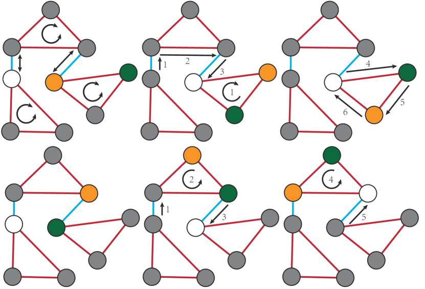
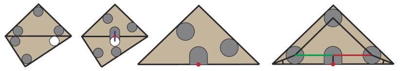
where each pair of positions in a sub-swap are connected directly by some , where is either a loop edge or an inter-cell edge. In either case, the sub-swap can be performed with the help of a nearby vacant vertex as illustrated in Figure 2. Finally, such vacant vertex must exist because our number of robots is strictly less than the number of vertices and the vacant position can be moved anywhere via vacant moves.
IV-B Parallel Robot Moves
![[Uncaptioned image]](https://cdn.awesomepapers.org/papers/1ac95a38-d211-4e7a-bc4c-1eb299786696/x2.png)
In the worst case, the makespan of above mentioned MPP solutions is . This is because we have only one vacant vertex, which is needed to perform every sub-swap. When more vacant vertices are available, we can parallelize the sub-swaps and improve the makespan. We present a space-time search algorithm to find parallel sub-swaps, which is similar to [15] in principle but adapted to graphs of more general topology. As illustrated in the inset, we first use the CLINK algorithm [32] to cluster the loops into a binary tree. This algorithm starts by treating each loop as a separate cluster, and then iteratively merge two smallest clusters (with the smallest number of vertices) until only one cluster is left. We then iteratively merge small leaf nodes until all leaf nodes have more than loops ( in the inset), where is a user specified parameter determining the congestion-level. In the worst case, this method requires vertices to be left vacant. Next, we introduce a vacant vertex for each leaf node. As a result, cyclic moves and vacant moves can be performed parallelly within a leaf node and two pairs of connected leaf nodes can perform two robot position swaps in parallel. Finally, we adopt the divide-and-conquer algorithm proposed in [15]. For every internal binary tree node, we consider their two children, which are two connected sub-graph. We swap robots between the two sub-graphs until and belongs to the same sub-graph for all . This procedure is performed recursively from the root node to all the leaves, where the swaps within different sub-trees are performed in parallel.
IV-C Scheduling Robot Swaps between Sub-Graphs
The major challenging in the above algorithm lies in the scheduling of parallel robot position swaps between sub-graphs, for which we use a space-time data structure. We denote as the th leaf node and we assume there are leaf nodes in one of the sub-graph and in the other (). The inter-sub-graph position swaps are decomposed into several rounds, where each round consists of several parallel position swaps between two connected leaf nodes. We denote as as the state of at the beginning of th round. We further connect and using a space-time edge if two conditions hold: 1) and are connected by some inter-loop edge ; 2) and belongs to the same sub-graph, i.e., or . Our space-time data structure is defined as the space-time graph , where is the maximal allowed number of rounds. Note that the space-time graph is directed with each directing from to . The inter-sub-graph position swaps can be accomplished by multi-rounds of swaps between leaf nodes, which in turn corresponds to selecting a set of space-time edges . Our algorithm greedily select a set of space-time edges leading to an inter-sub-graph position swap in the earliest round. After each selection, we remove the conflicting space-time edges before selecting the next set of edges, until all the robots belong to the correct sub-graph. When no position swaps can be found for the given , we introduce a new round and increase by one. This procedure is guaranteed to terminate.
Our method is outlined in Algorithm 1, which is composed of two main steps. First, we consider all pairs of connected leave nodes belonging to different sub-graphs. We find the two shortest paths connecting from , to some leaf node containing a robot that belongs to a different sub-graph. Specifically, we run Dijkstra’s algorithm with all-one edge weights from both and . We terminate the Dijkstra’s algorithm at any satisfying the following condition:
| (1) |
where we define as the number of robots within that belongs to a different sub-graph from at the beginning of the th round. Intuitively, Equation 1 ensures that swapping one more robot away from during the th round will not cause conflict with the number of to-be-swapped robots required by other swapping operations in the future rounds. Finally, note that we consider nodes pairs in a time-ascending order. The first pair of leaf nodes, for which such paths can be found, are selected, which corresponds to the position swap in the earliest round.
Our second step would remove three types of conflicting edges: 1) If an edge is selected, then all the edges are removed because they conflict with the edges along the two paths; 2) all the edges are removed because they conflict with the inter-sub-graph swap between , ; 3) Let’s define as the number of robots belonging to the same sub-graph as at the beginning of th round ( equals to the number of vertices in ), then all the edges:
should be removed. This is because selecting edge implies that a robot must be swapped with another robot at th round. We must have belongs to the same sub-graph as at the beginning of th round, because otherwise the shortest path would stop at instead of moving on to . However, implies that, if was swapped out of during th round, there will not be enough to-be-swapped agents (that belongs to the same sub-graph as ) during some future rounds.
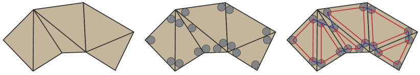
V Graph Embedding and Mesh Discretization
In this section, we move on to consider the geometric properties of that allows robots to move in a collision-free manner within a of arbitraily complex geometry. Our key innovation is a mapping from a mesh discretizing to a graph embedded in . As illustrated in Figure 3 (a), a mesh discretizing , denoted as , is another graph that is also a simplicial-complex, cell-decomposition of and we denote all the variables defined on the mesh using a bar over variables. Given a mesh , we can convert it into a graph using Algorithm 2, which is denoted as a mapping . Algorithm 2 consists of 4 general steps. First, we place robots on inner corner points of each cell, i.e. points inside a cell that are distance- away from two consecutive edges of the cell. Next, we assume that 3 robots inside the same cell form a loop, along which cyclic moves can be performed, and we add 3 loop edges to . We then add inter-cell edges to between the two pairs of corner points sharing an edge in , along which vacant move can be performed. Note that some cells may be too small and robots placed on inner corners are not collision-free. Even when corner points are collision-free, robots inside the same cell can still collide when performing cyclic moves. Therefore, we add a fourth and final step to remove from all the corner points (and incident edges) in invalid cells. We define a cell as invalid if the 3 corner points or cyclic moves are not collision-free. In the following, we show that the collision-free conditions of can be converted to three differentiable geometric constraints on .
V-A Condition 1: Planner Embedding
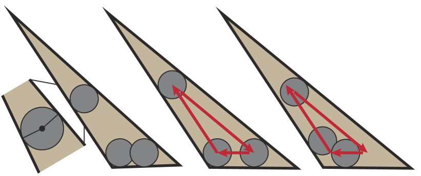
Since is a simplicial complex, each cell is a triangle and we denote the 3 vertices of this triangle as: . The distance- corner points can be computed using the following formula, as illustrated in Figure 4 (a):
| (2) |
We only show formula for and the formulas for are symmetric. We will mark the cell as invalid and remove the 3 vertices from if there are overlappings between .
V-B Condition 2: Collision-Free Cyclic Moves
Even when the 3 corner points are not overlapping, robots can still collide when they perform cyclic moves along the 3 loop edges with constant speed, as illustrated in Figure 4 (b). To derive a condition for collision-free cyclic moves, we assume that the 3 robots trace out a trajectory where . At time , the 3 robots are at positions:
and we have collision-free cyclic moves if:
| (3) |
Here we use cyclic subscripts to denote 3 symmetric conditions. The left-hand side of Equation 3 is quadratic when squared and determining the smallest value of a quadratic equation in has closed-form solution, which can be used for determining whether a cell is invalid in Algorithm 2.
In addition to determining the validity of a cell, our mesh optimization algorithm (Section VI) requires an operator that can modify an invalid cell’s geometric shape to achieve validity using numerical optimization. To this end, we derive a condition equivalent to Equation 3 but does not contain continuous time variable , because the variable can take infinitely many values from leading to a difficult semi-infinite programming problem [33]. Taking one of the equations in Equation 3 for example (the other 2 cases are symmetric), its left-hand-side is a polynomial of a single time variable . To eliminate , the Fekete, Markov-Lukaćz theorem [34] can be applied to show that, if Equation 3 holds, then we have:
where are four unknown variables to be fitted. The PSD-cone constraint is equivalent to two quadratic constraints: and . By equating coefficients in the quadratic constraints, we can express in terms of to get the following equivalent form:
| (4) | ||||
where is an additional decision variable that cannot be eliminated. But unlike , we only need to satisfy Equation LABEL:eq:equi_cond2 for a single . We summarize this result below:
V-C Condition 3: Collision-Free Vacant Moves
We show that, as long as condition 2 is satisfied, condition 3 must also be satisfied, so always satisfy condition 3. Condition 3 requires that a robot can move to a vacant position along any . We analyze two cases: being a loop edge or being an inter-cell edge.
Loop edge: If one of the 3 corner points in a cell is vacant and another robot is moving along a loop edge to , we show that this move is always collision-free. We prove by contradiction as illustrated in Figure 5. If this move is not collision-free, then the third corner point must be in the way between and . However, in this case, cyclic moves in the cell is not collision-free, which contradicts condition 2.
Inter-cell edge: If two neighboring triangles satisfy condition 2 and share an edge , then cyclic moves inside each triangle are collision-free. As illustrated in Figure 6, if robot is to be moved to a vacant position along an inter-cell edge, then we can rotate (along with the two other robots) clockwise and counterclockwise until the line-segment is orthogonal to and the convex hull of and does not contain other agents so the vacant move is collision-free. We prove in Appendix IX that such convex hull always exists between any pair of valid triangles. Finally, we rotate reversely to undo extra changes.
VI Mesh Optimization
In this section, we present a variant of mesh optimization algorithm [19, 35] to search for that maximizes a user given metric . Afterwards, a corresponding can be extracted using Algorithm 2 to solve for MPP problems.
VI-A Metric Function
Our metric consists of 4 terms that can either be a function of the mesh or the graph . These four terms measure the robot packing density as well as the area covered by the robots in . Our first term, is defined as: , which is the number of vertices contained in . This term reflects the number of robots that can hold, but MPP problems might not be feasible for all these robots because might not be connected. is a heuristic that guides our algorithm to find more valid cells at an early stage and then try to connect them. Our second term, , is the number of robots in the largest connected component of :
which is the maximal number of robots for which MPP problems are feasible. Note that are discrete, non-differentiable terms that are related to both the topology and geometry of . To increase , we need to update the shape of triangles in and also update their connectivity so that they are valid. Our third term is the agent packing density averaged over the valid cells:
is a heuristic guidance term that biases our algorithm towards denser robot packing, when only a subset of the workspace is covered by the robot. Our last metric term is the 2D AMIPS energy [36] using the smallest regular triangle satisfying condition 2 as the target shape. is differentiable, purely geometric, and related to only.
VI-B Greedy Maximization of Metric
The greedy algorithm is summarized in Algorithm 3, which exhaustively tries one of the re-meshing operators: edge-flip, edge-split, edge-collapse, vertex-smoothing, local-optimization, and global-optimization. Our re-meshing operators, except for global-optimization, are all local and only affect a small neighborhood of cells. The first 4 re-meshing operators are inherited from [19, 35], as illustrated in Figure 7. Edge-flip is guided by and is mostly applied to obtuse triangles and turns them into acute triangles. Edge-split and edge-collapse are used to remove tiny edges and split long edges in , respectively. Finally, vertex-smoothing locally optimizes with respect to the one-ring neighborhood of a single vertex. The four operators combined can turn a low-quality mesh into one with nice element shapes.
Our algorithm uses two passes. In the first pass, we allow the algorithm to explore a larger search space by allowing both edge-collapse and edge-split. To ensure the convergence of the first pass, we avoid the cases where consecutive edge-flip and edge-split operators happen for a same edge repeatedly. Allowing edge-split will create more triangles and potentially lead to denser packing of robots. In practice, we split a when its length is larger than of the optimal length . Here the optimal length is the edge length of the smallest regular triangles satisfying condition 2, which equals to: . In the second pass, we are more conservative and disallow edge-split. This pass can be considered as post-processing, merging too small triangles and simplifying the robot layout. Within each pass, we check every possible operator and only accept operators when the weighted metric monotonically increases and we set . We also reject operators that violate our assumption on being a cell decomposition, i.e. introducing non-manifold connection and flipped cells. The non-manifoldness of can happen only in edge-collapse and can be avoided by the link condition check [37]. A flipped cell has a negative area which can be checked by the following constraint:
| (5) |
VI-C Local- and Global-Optimization Operators
Aside from the four remeshing operators inherited from [19, 35], we introduce one local- and one global-optimization operators. These operators use the primal-dual interior point method to optimize the geometric shape of the cells, taking condition 2 as hard constraints. At the same time, we maximize by minimizing the area of valid cells, leading to a denser robot packing. Specifically, for a cell in with vertices , we solve the following problem in the local-optimization operator:
| (6) | ||||
where we require that the entire mesh to be a cell decomposition, so we add Equation 5 for all cells. We also require that those originally valid cells stay valid, so we add Equation LABEL:eq:equi_cond2 for all valid cells. This optimization can be solved efficiently because it is local. Since we only treat the 3 vertices of a single cell in as decision variables, most of the terms in the objective function and constraints are outside the 1-ring neighborhood of and not influenced by the decision variables, which can be omitted. Note that Equation LABEL:eq:equi_cond2 is expressed in terms of the corner points , instead of mesh vertices . When the optimizer requires partial derivatives of Equation LABEL:eq:equi_cond2 against , we use the chain rule on the relationship Equation 2.
The global-optimization operator is very similar to the local-optimization operator, which also takes the form of Equation 6, but we set all the variables as decision variables. The global-optimization is more expensive than all other operators, but we found that this last operator can significantly improve robot packing density and it is more efficient than applying the local-optimization operator to each of the cell.
VII Results and Analysis
We implement our algorithm and conduct experiments on a single desktop machine with Intel i7-9700 CPU. The input to our algorithm is a vector image in the svg format representing . Our main Algorithm 3 starts from an initial guess of , which can be generated using Triangle [38]. Our mesh optimization algorithm can nicely turn a triangle mesh (left of the inset), with an arbitrary initialization that has only few triangles satisfying the graph embedding constraints, into a regular triangle mesh (right of the inset) with most of its triangles being valid graph nodes for MPP problems.
![[Uncaptioned image]](https://cdn.awesomepapers.org/papers/1ac95a38-d211-4e7a-bc4c-1eb299786696/tri_tri.png)
We evaluate our algorithm on a set of complex workspaces and we summarize the statistics of , , robot density , free space coverage (the ratio between the area of all valid cells and the area of ), and computational time of the mesh optimization in Figure 8 and Table I.
| 1 | 2 | 3 | 4 | 5 | 6 | 7 | 8 | 9 | 10 | |
| 1489 | 1061 | 782 | 1021 | 756 | 569 | 1515 | 877 | 981 | 1104 | |
| 1489 | 1061 | 782 | 1021 | 756 | 569 | 1515 | 877 | 981 | 1104 | |
| 0.31 | 0.29 | 0.30 | 0.30 | 0.29 | 0.28 | 0.30 | 0.31 | 0.32 | 0.33 | |
| Coverage | 0.995 | 0.979 | 0.983 | 0.984 | 1.000 | 0.994 | 0.985 | 0.993 | 0.998 | 0.990 |
| time | 14133 | 2598 | 4439 | 5866 | 2793 | 3241 | 6155 | 2539 | 7836 | 9066 |
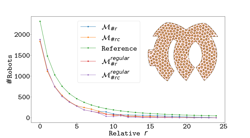
We also compare our method with the regular-pattern baseline, illustrated in Figure 1 and Figure 9. Using our arrangement of robots in Section V, we can use regular triangles with the optimal area to cover and then remove triangles that are outside . As shown in Figure 9, the regular pattern does lead to higher and when the size of a robot is small. But, as the robot size gets larger, our method can produce a graph embedding with a higher number of robots (Figure 1 and Figure 9). Moreover, regular pattern method introduces undesirable zig-zag boundary coverage (see Figure 1 for a visual comparison on a simple workspace).
We also profile the influence of different robot radius. In Figure 9, we change the radius , and compare the curve with the ideal curve by plotting the change of and against . Our method closely matches the ideal reference curve and the performance is comparable to regular-pattern baseline with different .
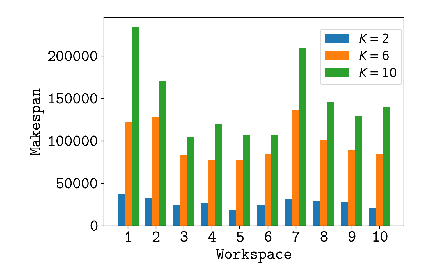
On the optimized and corresponding , we use our parallel MPP scheduler Algorithm 1 to solve randomized MPP problems for each of the environments listed in Figure 8 and Table I. We profile the rate of acceleration using more and more vacant vertices (determined by the parameter ). We summarize the average makespan for each environment for three different s in Figure 10. We observe greater makespan reductions as goes smaller that will consider more agents as vacant.
VIII Conclusion and Limitations
We present a method to solve graph-restricted MPP problems in complex environments. Our method uses a special graph topology to ensure MPP feasibility. Using a divide-and-conquer algorithm with space-time scheduling, we can parallelize the robot motions and greedily improve the makespan. The special graph topology can be further identified with triangular meshes, which in turn is optimized via mesh optimization and embedded into arbitrarily complex environments. In the future, we plan to extend our method to continuous robot motions under general dynamic constraints. \AtNextBibliography
References
- [1] R. Chinta, S. D. Han and J. Yu “Coordinating the Motion of Labeled Discs with Optimality Guarantees under Extreme Density” In The 13th International Workshop on the Algorithmic Foundations of Robotics, 2018
- [2] J. M. Palacios-Gasós et al. “Optimal path planning and coverage control for multi-robot persistent coverage in environments with obstacles” In 2017 IEEE International Conference on Robotics and Automation (ICRA), 2017, pp. 1321–1327 DOI: 10.1109/ICRA.2017.7989156
- [3] K. M. Hasan, Abdullah-Al-Nahid and K. J. Reza “Path planning algorithm development for autonomous vacuum cleaner robots” In 2014 International Conference on Informatics, Electronics Vision (ICIEV), 2014, pp. 1–6 DOI: 10.1109/ICIEV.2014.6850799
- [4] J. L. Baxter, E. K. Burke, J. M. Garibaldi and M. Norman “Multi-Robot Search and Rescue: A Potential Field Based Approach” In Autonomous Robots and Agents Berlin, Heidelberg: Springer Berlin Heidelberg, 2007, pp. 9–16
- [5] John E Hopcroft, Jacob Theodore Schwartz and Micha Sharir “On the Complexity of Motion Planning for Multiple Independent Objects; PSPACE-Hardness of the” Warehouseman’s Problem”” In The international journal of robotics research 3.4 Sage Publications Sage CA: Thousand Oaks, CA, 1984, pp. 76–88
- [6] Paul Spirakis and Chee K Yap “Strong NP-hardness of moving many discs” In Information Processing Letters 19.1 Elsevier, 1984, pp. 55–59
- [7] Glenn Wagner, Minsu Kang and Howie Choset “Probabilistic path planning for multiple robots with subdimensional expansion” In 2012 IEEE International Conference on Robotics and Automation, 2012, pp. 2886–2892 IEEE
- [8] Gildardo Sánchez and Jean-Claude Latombe “On Delaying Collision Checking in PRM Planning: Application to Multi-Robot Coordination” In The International Journal of Robotics Research 21.1, 2002, pp. 5–26
- [9] Duong Le and Erion Plaku “Cooperative Multi-Robot Sampling-Based Motion Planning with Dynamics” In ICAPS, 2017
- [10] Guni Sharon, Roni Stern, Ariel Felner and Nathan R Sturtevant “Conflict-based search for optimal multi-agent pathfinding” In Artificial Intelligence 219 Elsevier, 2015, pp. 40–66
- [11] Vincenzo Auletta, Angelo Monti, Mimmo Parente and Pino Persiano “A linear-time algorithm for the feasibility of pebble motion on trees” In Algorithmica 23.3 Springer, 1999, pp. 223–245
- [12] R. Luna and K. E. Bekris “Push and Swap: Fast Cooperative Path-Finding with Completeness Guarantees” In International Joint Conferences in Artificial Intelligence (IJCAI-11), 2011, pp. 294–300
- [13] Jingjin Yu and Daniela Rus “Pebble motion on graphs with rotations: Efficient feasibility tests and planning algorithms” In Algorithmic foundations of robotics XI Springer, 2015, pp. 729–746
- [14] Shuai D. Han, Edgar J. Rodriguez and Jingjin Yu “SEAR: A Polynomial- Time Multi-Robot Path Planning Algorithm with Expected Constant-Factor Optimality Guarantee.” In 2018 IEEE/RSJ International Conference on Intelligent Robots and Systems, IROS 2018, Madrid, Spain, October 1-5, 2018 IEEE, 2018
- [15] J. Yu “Average Case Constant Factor Time and Distance Optimal Multi-Robot Path Planning in Well-Connected Environments” In Autonomous Robots, 2019
- [16] J. Yu and S. M. LaValle “Optimal Multi-Robot Path Planning on Graphs: Complete Algorithms and Effective Heuristics” In IEEE Transactions on Robotics 32.5, 2016, pp. 1163–1177
- [17] Liang He, Zherong Pan, Biao Jia and Dinesh Manocha “Efficient Multi-Agent Motion Planning in Continuous Workspaces Using Medial-Axis-Based Swap Graphs” In arXiv:2002.11892 arXiv:2002.11892, 2020
- [18] Hugues Hoppe “New quadric metric for simplifying meshes with appearance attributes” In Proceedings Visualization’99 (Cat. No. 99CB37067), 1999, pp. 59–510 IEEE
- [19] Hugues Hoppe et al. “Mesh optimization” In Proceedings of the 20th annual conference on Computer graphics and interactive techniques, 1993, pp. 19–26
- [20] Jur Berg, Jack Snoeyink, Ming Lin and Dinesh Manocha “Centralized path planning for multiple robots: Optimal decoupling into sequential plans” In Robotics: Sciences and Systems, 2009 DOI: 10.15607/RSS.2009.V.018
- [21] Pierre Alliez, Giuliana Ucelli, Craig Gotsman and Marco Attene “Recent advances in remeshing of surfaces” In Shape analysis and structuring Springer, 2008, pp. 53–82
- [22] Bryan E. Feldman, James F. O’Brien and Bryan M. Klingner “Animating Gases with Hybrid Meshes” In Proceedings of ACM SIGGRAPH 2005, 2005 URL: http://graphics.cs.berkeley.edu/papers/Feldman-AGH-2005-08/
- [23] Julien Villard and Houman Borouchaki “Adaptive meshing for cloth animation” In Engineering with Computers 20.4 Springer, 2005, pp. 333–341
- [24] Frank Lingelbach “Path planning using probabilistic cell decomposition”, 2005
- [25] Jean-Claude Latombe “Exact cell decomposition” In Robot Motion Planning Springer, 1991, pp. 200–247
- [26] A. Li, L. Wang, P. Pierpaoli and M. Egerstedt “Formally Correct Composition of Coordinated Behaviors Using Control Barrier Certificates” In 2018 IEEE/RSJ International Conference on Intelligent Robots and Systems (IROS), 2018, pp. 3723–3729 DOI: 10.1109/IROS.2018.8594302
- [27] Geunho Lee, Nak Young Chong and Henrik Christensen “Adaptive triangular mesh generation of self-configuring robot swarms” In 2009 IEEE International Conference on Robotics and Automation, 2009, pp. 2737–2742 IEEE
- [28] Petra Mutzel and René Weiskircher “Bend minimization in orthogonal drawings using integer programming” In International Computing and Combinatorics Conference, 2002, pp. 484–493 Springer
- [29] Andreas Fischer et al. “Virtual network embedding: A survey” In IEEE Communications Surveys & Tutorials 15.4 IEEE, 2013, pp. 1888–1906
- [30] Chi-Han Peng, Yong-Liang Yang and Peter Wonka “Computing layouts with deformable templates” In ACM Transactions on Graphics (TOG) 33.4 ACM New York, NY, USA, 2014, pp. 1–11
- [31] Chi-Han Peng, Helmut Pottmann and Peter Wonka “Designing Patterns Using Triangle-Quad Hybrid Meshes” In ACM Trans. Graph. 37.4 New York, NY, USA: Association for Computing Machinery, 2018 DOI: 10.1145/3197517.3201306
- [32] Daniel Defays “An efficient algorithm for a complete link method” In The Computer Journal 20.4 Oxford University Press, 1977, pp. 364–366
- [33] Ankur Sinha, Pekka Malo and Kalyanmoy Deb “A review on bilevel optimization: from classical to evolutionary approaches and applications” In IEEE Transactions on Evolutionary Computation 22.2 IEEE, 2017, pp. 276–295
- [34] Monique Laurent “Sums of squares, moment matrices and optimization over polynomials” In Emerging applications of algebraic geometry Springer, 2009, pp. 157–270
- [35] Yixin Hu et al. “Tetrahedral Meshing in the Wild” In ACM Trans. Graph. 37.4 New York, NY, USA: Association for Computing Machinery, 2018 DOI: 10.1145/3197517.3201353
- [36] Xiao-Ming Fu, Yang Liu and Baining Guo “Computing Locally Injective Mappings by Advanced MIPS” In ACM Trans. Graph. 34.4 New York, NY, USA: Association for Computing Machinery, 2015
- [37] Tamal K. Dey, Herbert Edelsbrunner, Sumanta Guha and Dmitry V. Nekhayev “Topology Preserving Edge Contraction” In Publ. Inst. Math. (Beograd) (N.S 66, 1998, pp. 23–45
- [38] Jonathan Richard Shewchuk “Triangle: Engineering a 2D quality mesh generator and Delaunay triangulator” In Applied Computational Geometry Towards Geometric Engineering Berlin, Heidelberg: Springer Berlin Heidelberg, 1996, pp. 203–222
- [39] K Hägglöf, Per Olov Lindberg and Lars Svensson “Computing global minima to polynomial optimization problems using Gröbner bases” In Journal of global optimization 7.2 Springer, 1995, pp. 115–125
- [40] Jinhu Li and Jeffrey S Racine “Maxima: An open source computer algebra system” JSTOR, 2008
IX Appendix: Proof of Vacant Move
Lemma IX.1
Assuming condition 2 of Section V, for a pair of positions in different triangles sharing an edge , and can be rotated such that the convex hull of and does not contain other agents.
Proof:
As illustrated in Figure 11 (ab), we have to align and by rotating clockwise and counterclockwise. We choose to always rotate until the edge between and passes through the center of the shared edge: in Figure 11 (c). Therefore, we only need to consider one triangle and show that the half capsule lies inside the triangle (Figure 11 (c)), for which an equivalent condition is and in Figure 11 (d) for all possible choices of .
We first derive closed-form expressions for . Note that at least one of the two angles are acute and, without loss of generality, we assume that is acute. We further denote and . Condition 2 implies the following two conditions:
| (7) | ||||
| (8) |
Since is an acute angle, it is easy to show that attains its minimal value when . Therefore, we can eliminate and derive a lower bound of from Equation 7 (This is lower bound because Equation 8 is omitted). After trigonometric simplification, we can express the lower bound of as the following functions of :
To show that is always positive, we define and show that is always larger than zero on the following semi-algebraic set:
Note that is a polynomial function and verifying the positivity of a polynomial function on a semi-algebraic set can be performed analytically using Gröbner basis [39]. We use the computational algebraic software Maxima [40] to verify that the global minimum of on is zero. Therefore, we conclude that for any valid triangles. Similarly, we can derive the lower bound of resulting in a similar formula:
If we define and compute the global minimum of on , the result is negative. Therefore, we need to consider two cases separately. First, if , then we have the following semi-algebraic set:
The global minimum of on is zero. Therefore, we conclude that holds for any valid triangles with . If , then the third angle is acute and we can show that the left-hand side of Equation 8 attains its minimum when . As a result, Equation 8 gives us another lower bound for . Applying trigonometric simplification and we have:
If we define , we can show that the global minimum of on is zero. As a result, for any valid triangles with . ∎