NewReferences
Multi-rubric Models for Ordinal Spatial Data with Application to Online Ratings Data
Abstract
Interest in online rating data has increased in recent years in which ordinal ratings of products or local businesses are provided by users of a website, such as Yelp! or Amazon. One source of heterogeneity in ratings is that users apply different standards when supplying their ratings; even if two users benefit from a product the same amount, they may translate their benefit into ratings in different ways. In this article we propose an ordinal data model, which we refer to as a multi-rubric model, which treats the criteria used to convert a latent utility into a rating as user-specific random effects, with the distribution of these random effects being modeled nonparametrically. We demonstrate that this approach is capable of accounting for this type of variability in addition to usual sources of heterogeneity due to item quality, user biases, interactions between items and users, and the spatial structure of the users and items. We apply the model developed here to publicly available data from the website Yelp! and demonstrate that it produces interpretable clusterings of users according to their rating behavior, in addition to providing better predictions of ratings and better summaries of overall item quality.
Key words and phrases: Bayesian hierarchical model; data augmentation; nonparametric Bayes; ordinal data; recommender systems; spatial prediction.
1 Introduction
In recent years, the complexity of data used to make decisions has increased dramatically. A prime example of this is the use of online reviews to decide whether to purchase a product or visit a local business; we refer to the objects being reviewed as items. Consider data provided by Yelp! (see, http://www.yelp.com/), which allows users to rate items, such as restaurants, convenience stores, and so forth, on a discrete scale from one to five “stars.” Additional features of the businesses are also known, such as the spatial location and type of business. Datasets of this type are typically very large and exhibit complex dependencies.
As an example of this complexity, users of Yelp! effectively determine their own standards when rating a local business. We refer to the particular standards a user applies as a rubric. We might imagine a latent variable representing the utility, or benefit, user obtained from item . For a given level of utility, however, different users may still give different ratings due to having different standards for the ratings; for example, one user may rate a restaurant 5 stars as long as it provides a non-offensive experience, a second user might require an exceptional experience to rate the same restaurant 5 stars, and a third user may rate all items with star in order to “troll” the website. Each of these users are applying different rubrics in translating their utility to a rating for the restaurant. In addition we also expect user-specific selection bias in the sense that some users may rate every restaurant they attend, while other users may only rate restaurants that they feel strongly about.
This article makes several contributions. First, we develop a semiparametric Bayesian model which accounts for the existence of multiple rubrics for ratings data that are observed over multiple locations. To do this, we use a spatial cumulative probit model (e.g., see Higgs and Hoeting,, 2010; Berret and Calder,, 2012; Schliep and Hoeting,, 2015) in which the break-points are modeled as user-specific random effects. This requires a flexible model for the distribution of the random effects, which we model as a discrete mixture. A by-product of our approach is that we obtain a clustering of users according to the rubrics they are using.
Second, we use the multi-rubric model to address novel inferential questions. For example, ratings provided to a user might be adjusted to match that user’s rubric, or to provide a distribution for the rating that a user would provide conditional on having a particular rubric. Utilizing this user-specific standardization of ratings may provide users with better intuition for the overall quality of an item.
This adjustment of restaurant quality for the rubrics is similar to, but distinct from, the task of predicting a user’s ratings. Good predictive performance is required for filtering, which refers to the task of processing the rating history of a user and producing a list of recommendations (for a review, see Bobadilla et al.,, 2013). As a third contribution, we show that allowing for multiple rubrics improves predictions.
The model proposed here also has interesting statistical features. A useful feature of our model is that it allows for more accurate comparisons across items. For example, if a user rates all items with star, then the model discounts this user’s ratings. This behavior is desirable for two reasons. First, if a user genuinely rates all items with star, then their rating is unhelpful. Second, it down-weights the ratings of users who are exhibiting selection bias and only rating items which they feel strongly about, which is desirable as comparisons across items will be more indicative of true quality if they are based on individuals who are not exhibiting large degrees of selection bias.
Additionally, the rubrics themselves may be of intrinsic interest. We demonstrate that the rubrics learned by our model are highly interpretable. For example, when analyzing the Yelp! dataset in Section 4, we obtain Figure 7 which displays the ratings observed for users assigned to a discrete collection of rubrics and reveals several distinct rating patterns displayed by users.
Other features of our model are also of potentially independent interest. The multi-rubric model can be interpreted as a novel semiparametric random-effects model for ordinal data, even for problems in which the intuition behind the multi-rubric model in terms of latent utility does not hold. Other study designs in which the multi-rubric analogy may be useful include longitudinal survey studies, or more general ordinal repeated-measures designs. Additionally, the cumulative probit model we use to model latent user preferences includes a spatial process to account for spatial dependencies across local businesses. Recovering an underlying spatial process allows for recommending entire regions to visit, rather than singular items. The development of low-rank spatial methodology for large-scale dependent ordinal data is of interest within the spatial literature, as the current spatial literature for ordinal data do not typically address large datasets on a similar order of the Yelp! dataset (e.g., see De Oliveira,, 2004, 2000; Chen and Dey,, 2000; Cargnoni et al.,, 1997; Knorr-Held,, 1995; Carlin and Polson,, 1992; Higgs and Hoeting,, 2010; Berret and Calder,, 2012; Velozo et al.,, 2014, among others). We model the underlying spatial process using a low-rank approximation (Cressie and Johannesson,, 2008) to a desired Gaussian process (Banerjee et al.,, 2008; Bradley et al.,, 2015).
Starting from Koren and Sill, (2011), several works in the recommender systems literature have considered ordinal matrix factorization (OMF) procedures which are similar in many respects to our model (see also Paquet et al., 2012 and Houlsby et al., 2014). Our work differs non-trivially from these works in that the multi-rubric model treats the break-points as user-specific random effects, with a nonparametric prior used for the random effects distribution . For the Yelp! dataset, this extra flexibility leads to improved predictive performance. Additionally, our focus in this work extends to inferential goals beyond prediction; for example, depending on the distribution of the rubrics of users who rate a given item, the estimate of overall quality for that item can be shrunk to a variety of different centers, producing novel multiple-shrinkage effects. Several works in the Bayesian nonparametric literature have also considered flexible models for random effects in multivariate ordinal models (Kottas et al.,, 2005; DeYoreo and Kottas,, 2014; Bao and Hanson,, 2015), but do not treat the break-points themselves as random effects.
The paper is organized as follows. In Section 2, we develop the multi-rubric model, with an eye towards the Yelp! dataset, and provide implementation details. In Section 3, we illustrate the methodology on synthetic data designed to mirror features of the Yelp! dataset, and demonstrate that we can accurately recover the number and structure of the rubrics when the model holds, as well as effectively estimate the underlying latent utility field. In Section 4, we illustrate the methodology on the Yelp! dataset. We conclude with a discussion in Section 5. In supplementary material, we present simulation experiments which demonstrate identifiability of key components of the model.
2 The Multi-rubric model
2.1 Preliminary notation
We consider ordinal response variables taking values in . In the context of online ratings data, represents the rating that user provides for item . In the context of survey data, on the other hand, might represent the response subject gives to question . We do not assume that is observed for all pairs, but instead we observe , where is the total number of subjects and is the total number of items. For fixed we let be the set of users that rate item , and similarly for fixed we let be the set of items that user rates.
2.2 Review of Cumulative Probit Models
Cumulative probit models (Albert and Chib,, 1993, 1997) provide a convenient framework for modeling ordinal rating data. Consider the univariate setting, with ordinal observations taking values in . We assume that is a rounded version of a latent variable such that if . Here, are unknown break-points. When has the Gaussian distribution this leads to the ordinal probit model, where .
We assume , as the variance of is confounded with the break-points . Any global intercept term is also confounded with the ’s; there are two resolutions to this issue. The first is to fix one of the ’s, e.g., . The second is to exclude an intercept term from . While the former approach is often taken (Albert and Chib,, 1997; Higgs and Hoeting,, 2010), it is more convenient in the multi-rubric setting to use the latter approach to avoid placing asymmetric restrictions on the break-points.
The ordinal probit model is convenient for Bayesian inference in part because it admits a simple data augmentation algorithm which iterates between sampling for and, assuming a flat prior for , sampling where has row and . Here, denotes the Gaussian distribution truncated to the interval . Additionally, an update for is needed. Efficient updates for can be implemented by using a Metropolis-within-Gibbs step to update as a block (for details, see Albert and Chib,, 1997, as well as Cowles,, 1996 for alternative MCMC schemes).
2.3 Description of the proposed model
2.3.1 The multi-rubric model
We develop an extension of the cumulative probit model to generic repeated-measures ordinal data . Following Albert and Chib, (1997) we introduce latent utilities , but specify a generic ANOVA model
| (1) |
where and are main effects and is an interaction effect. The multi-rubric model modifies the cumulative probit model by replacing the break-point parameter with -specific random effects with for some unknown . As before, we let if .
For concreteness, we take to be a finite mixture for some large , with and , where is a point-mass distribution at . We note that it is also straight-forward to use a nonparametric prior for such as a Dirichlet process (Escobar and West,, 1995; Ferguson,, 1973). We refer to the random effects as rubrics. Note that for each subject there exists a latent class such that .
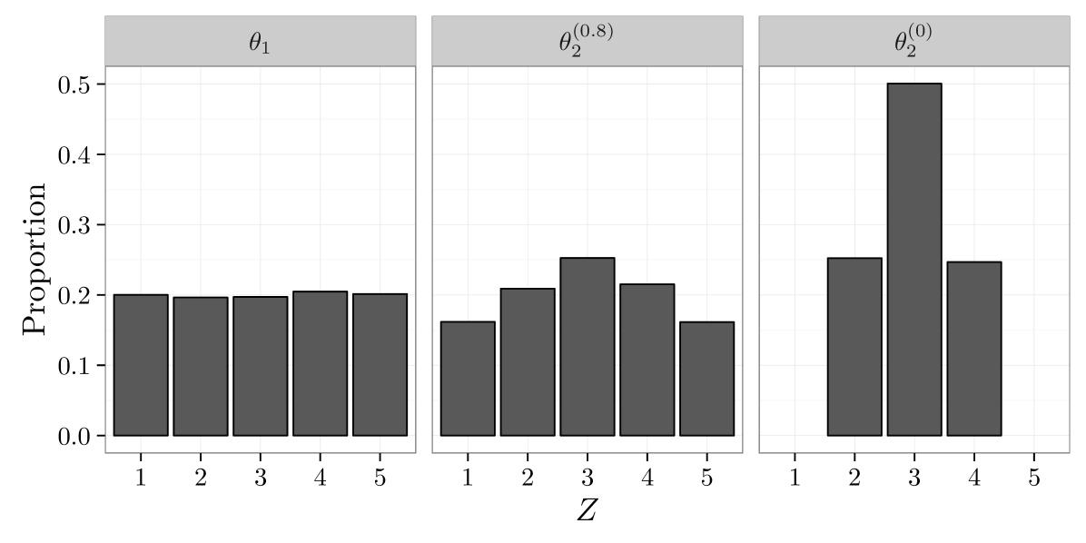
Figure 1 displays the essential idea for the model. Viewing as a latent utility, the rubric that the user is associated to leads to different values of the observed rating . In this example, the second rubric is associated to users who rate many items with a , while the first rubric is associated to users who do not rate many items with a .

Treating the break-points as random effects has several benefits. First, it offers additional flexibility over approaches for ordinal data which incorporate a random intercept (Gill and Casella,, 2009). Due to the fact that the ’s are confounded with both the location and scale of , treating the break-points as random effects is at least as flexible as treating the location and scale of the distribution of the ’s as random effects. We require this additional flexibility, as merely treating the location and scale of the ’s as random effects does not allow for the variety of rating behaviors exhibited by users. By treating the break-points as random effects, we are able to capture any distribution of ratings in a given rubric (see, e.g., Figure 7). In addition to flexibility, specifying as a discrete mixture induces a clustering of users into latent classes. To each user we associate a latent variable such that if . As will be demonstrated in Section 4, the latent classes of users discovered in this way are highly interpretable.
2.3.2 Model for the Yelp! data
Our model for the Yelp! data takes where
This is model (1) with , , and removed. This model can be motivated as a combination of the fixed-rank kriging approach of Cressie and Johannesson, (2008) with the probabilistic matrix factorization approach of Salakhutdinov and Mnih, (2007). The terms , , and are used to account for heterogeneity in the items. The term accounts for known covariates associated to each item. The term is used to capture spatial structure, and is modeled with a basis function expansion where denotes the longitude-latitude coordinates associated to the item and is a vector of basis functions. We note that it is straight-forward to replace our low-rank approach for with more elaborate approaches such as the full-scale approach of Sang and Huang, (2012). The term is an item-specific random effect which is used to capture item heterogeneity which cannot be accounted for by the covariates or the low-rank spatial structure.
The vectors and intuitively correspond to unmeasured user-specific and item-specific latent features. The term is large/positive when and point in the same direction (i.e., the user’s preferences align with the item’s characteristics), and is large/negative when and point in opposite directions. This allows the model to account not only for user-specific biases () and item-specific biases , but also interaction effects.
The multi-rubric model can be summarized by the following hierarchical model. For each model, we implicitly assume the statements hold conditionally on all variables in the models below, and that conditional independence holds within each model unless otherwise stated.
- Response model:
-
with probability and .
- Random effect model:
-
, , , and .
- Spatial process model:
-
where .
- Parameter model:
-
and where and .
To complete the model we must specify values for the hyperparameters , and , as well as the number of rubrics and the number of latent factors . In our illustrations we place half-Gaussian priors for the scale parameters, with , and . We let and set . Here, denotes a standard Gaussian distribution truncated to the positive reals. For a discussion of prior specification for variance parameters, see Gelman et al., (2006) and Simpson et al., (2017).
In our illustrations we use . For the Yelp! dataset, the choice of rubrics is conservative, and by setting for some fixed , we encourage to be nearly-sparse (Ishwaran and Zarepour,, 2002; Linero,, 2016). This strategy effectively lets the data determine how many rubrics are needed, as the prior encourages if rubric is not needed. The prior for is chosen to have density so that has the distribution of the order statistics of independent variables.
2.4 Evaluating item quality
A commonly used measure of item quality is the average rating of a user from the population where . This quantity is given by
Using properties of the Gaussian distribution, and recalling that , it can be shown that
| (2) |
where . In Section 4, we demonstrate the particular users who rated item exert a strong influence on the ’s, particularly for restaurants with few ratings.
Rather than focusing on an omnibus measure of overall quality, we can also adjust the overall quality of an item to be rubric-specific. This amounts to calculating which represents the average rating of item if all used rubric . Similar to (2), this quantity can be computed as
| (3) |
In Section 4, we use both (2) and (3) to understand the statistical features of the multi-rubric model.
2.5 Implementation Details
We use the reduced rank model where has row given by . We choose so that is an optimal low-rank approximation to where is associated to a target positive semi-definite covariogram. This is accomplished by taking composed of the first columns of where is the spectral decomposition of . The Eckart-Young-Mirsky theorem states that this approximation is optimal with respect to both the operator norm and Frobenius norm (see, e.g., Rasmussen and Williams,, 2005, Chapter 8). A similar strategy is used by Bradley et al., (2016, 2015), who use an optimal low-rank approximation of a target covariance structure where the basis is held fixed but is allowed to vary over all positive-definite matrices. In our illustrations, we use the squared-exponential covariance, i.e., (Cressie,, 2015).
To complete the specification of the model, we must specify the bandwidth , the number of latent factors , and the number of basis functions . We regard as a tuning parameter, which can be selected by assessing prediction performance on a held-out subset of the data. In principle, a prior can be placed on , however this results in a large computational burden; we instead evaluate several fixed values of chosen according to some rules-of-thumb and select the value with the best performance. For the Yelp! dataset, we selected , which corresponds undersmoothing the spatial field relative to Scott’s rule (see, e.g., Härdle and Müller,, 2000) by roughly a factor of two, and remark that substantively similar results are obtained with other bandwidths. Finally, can be selected so that the proportion of the variance in accounted for by the low-rank approximation exceeds some preset threshold; for the Yelp! dataset, we chose to account for 99% of the variance in .
When specifying the number of rubrics , we have found that the model is most reliable when is chosen large and for some ; under these conditions, the prior for is approximately a Dirichlet process with concentration and base measure (see, e.g., Teh et al.,, 2006). We recommend choosing to be conservatively large and allowing the model to remove unneeded rubrics through the sparsity-inducing prior on . We have found that taking large is necessary for good performance even in simulations in which the true number of rubrics is small and known.
We use Markov chain Monte Carlo to approximately sample from the posterior distribution of the parameters. A description of the sampler is given in the appendix.
2.6 A note on selection bias
Let if , and otherwise. In not modeling the distribution of , we are implicitly modeling the distribution of the ’s conditional on . When selection bias is present, this may be quite different than the marginal distribution of ’s. Experiments due to Marlin and Zemel, (2009) provide evidence that selection bias may be present in practice.
A useful feature of the approach presented here is that it naturally down-weights users who are exhibiting selection bias. For example, if user only rates items they feel negatively about, they will be assigned to a rubric for which is very large; this has the effect of ignoring their ratings, as there will be effectively no information in the data about their latent utility. As a result, when estimating overall item quality, the model naturally filters out users who are exhibiting extreme selection bias, which may be desirable.
In the context of prediction, the predictive distribution for should be understood as being conditional on the event ; that is, the prediction is made with the additional information that user chose to rate item . This is the case for nearly all collaborative filtering methods, as correcting for the selection bias necessitates collecting ’s for which would occurred naturally; for example, as done by Marlin and Zemel, (2009), we might assess selection bias by conducting a pilot study which forces users to rate items they would not have normally rated. With the understanding that all methods are predicting ratings conditional on , the results in Section 4 show that the multi-rubric model leads to increased predictive performance.
Selection bias should also be taken into account when interpreting the latent rubrics produced by our model. Our model naturally provides a clustering of users into latent classes, which we presented as representing differing standards in user ratings; however, we expect that the model is also detecting differences in selection bias across users. We emphasize that our goal is to identify and account for heterogeneity in rating patterns, and we avoid speculating on whether heterogeneity is caused by different rating standards or selection bias. For example, a user who rates items with only one-star or five-stars might be either (i) using a rubric which results in extreme behavior, with most of the break-points very close together; or (ii) actively choosing to rate items which they feel strongly about.
3 Simulation Study
The goal of this simulation is to illustrate that we can accurately learn the existence of multiple rubrics in settings where one would expect it would be difficult to detect them. We consider a situation where the data is generated according to two rubrics that are similar to each other. This allows us to assess the robustness of our model to various “degrees” of the multi-rubric assumption. The performance of our multi-rubric model is assessed relative to the single-rubric model, which is the standard assumption made in the ordinal data literature.
We calibrate components of the simulation model towards the Yelp! dataset to produce realistic simulated data. Specifically, we set and equal to the posterior means obtained from fitting the model to the Yelp! dataset in Section 4. We set , corresponding to a much stronger spatial effect than what was observed in the data, and for simplicity we removed the latent-factor aspect of the model by fixing . A two-rubric model is used with . We also use the same spatial basis functions and observed values of as in the Yelp! analysis in Section 4.
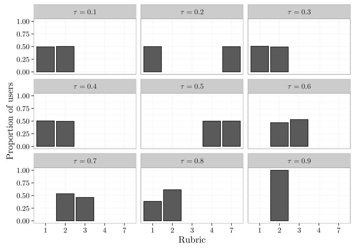
We now describe how the two rubrics and where chosen. First, was selected so that was evenly distributed among the five responses. Associated to is a probability vector . To specify , we use the same approach with a difference choice of . Let . Then is associated to in the same manner as is associated to . Here, indexes the similarity of and , and it can be shown that the total variation distance between the empirical distribution of and is . Thus, values of near correspond imply that the rubrics are similar, while values of near imply that they are dissimilar. Figure 2 presents the distribution of the ’s with when , and .
We fit a -rubric and single-rubric model for . Figure 3 displays the proportion of individuals assigned to each rubric for a given value of . If the model is accurately recovering the underlying rubric structure, we expect to see a half of the observations assigned to one rubric, and half to another; due to permutation invariance, which of the 10 rubrics is associated to and vary by simulation. Up to , the model is capable of accurately recovering the existence of two rubrics. We also see that, even at , the model accurately recovers the empirical distribution of the ’s associated to each rubric.
Next, we assess the benefit of using the multi-rubric model to predict missing values. For each value of , we fit a single-rubric and multi-rubric model. Using the same train-test split as in the our real data illustration, we compute the log likelihood on the held-out data which is further discussed in detail in Section 4 . Figure 4 shows the difference in held-out log likelihood for the single-rubric and multi-rubric model as a function of . Up-to , there is a meaningful increase in the held-out log-likelihood obtained from using the multi-rubric model. The case where is also particularly interesting, as this implies that the data were generated from the single rubric model. Here the predictive performance of our model at missing values appears to be robust to the case when the multiple rubric assumption is incorrect.
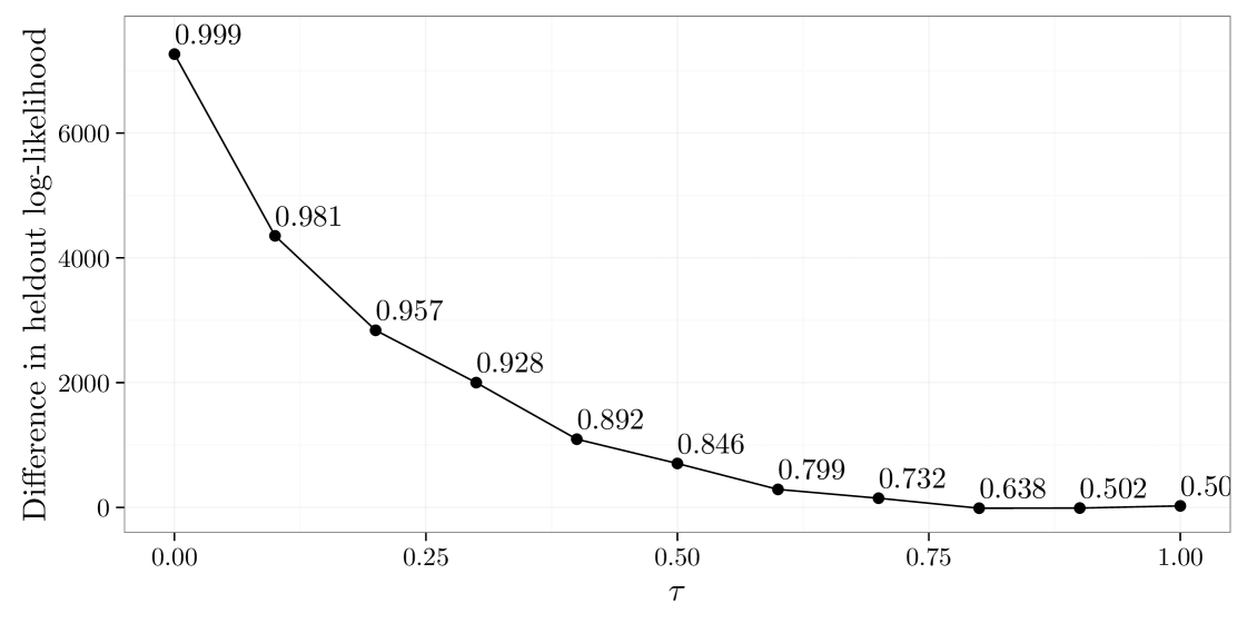
Displayed above each point in Figure 4 is the proportion of observations which are assigned to the correct rubric, where each observation is assigned to their most likely rubric. When the rubrics are far apart the model is capable of accurately assigning observations to rubrics. As the rubrics get closer together, the task of assigning observations to rubrics becomes much more difficult.
This simulation study suggests that the model specified here is able to disentangle the two-rubric structure, even when the rubrics are only subtly different. This leads to clear improvements in predictive performance for small and moderate values for . Additionally, when the multi-rubric assumption is negligible, or even incorrect, our model performs as well as the single-rubric model.
4 Analysis of Yelp data
We now apply the multi-rubric model to the Yelp! dataset, which is publicly available at https://www.yelp.com/dataset_challenge. We begin by preprocessing the data to include reviews only between January , 2013 and December 2016, and restrict attention to restaurants in Phoenix and its surrounding areas. We further narrow the data to include only users who rated at least 10 restaurants; this filtering is done in an attempt to minimize selection bias, as we believe that “frequent raters” should be less influenced by selection bias.
We first evaluate the performance of the single-rubric and multi-rubric models for various values of the latent factor dimension . We set and induce sparsity in by setting . We divide the indices into a training set and testing set of equal sizes by randomly allocating half of the indices to the training set. We evaluate predictions using a held-out log-likelihood criteria
| (4) | ||||
where , denotes the posterior predictive distribution of , and indexes the approximate draws from the posterior obtained by MCMC. Results for the values , and 5, over 10 splits into training and test data, are given in Figure 6. We also compare our methodology to ordinal matrix factorization (Paquet et al.,, 2012) with learned breakpoints and spatial smoothing, and the mixture multinomial model (Marlin and Zemel,, 2009) with mixture components. The multi-rubric model leads to an increase in the held-out data log-likelihood (4) of roughly over ordinal matrix factorization and over the mixture multinomial model. Additionally, we note that the holdout log-likelihood was very stable over replications. The single-rubric model is essentially equivalent to ordinal matrix factorization.
The dimension of the latent factors and has little effect on the quality of the model. We attribute this to the fact that and are typically small, making it difficult for the model to recover the latent factors. On other datasets where this is not the case, such as the Netflix challenge dataset, latent-factor models represent the state of the art and are likely essential for the multi-rubric model. In the supplementary material we show in simulation experiments that the ’s, ’s, and are identified.
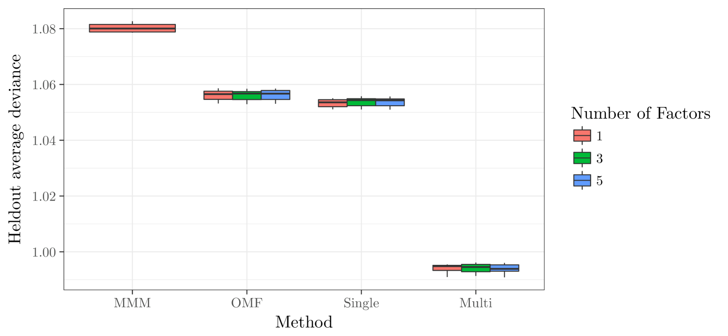
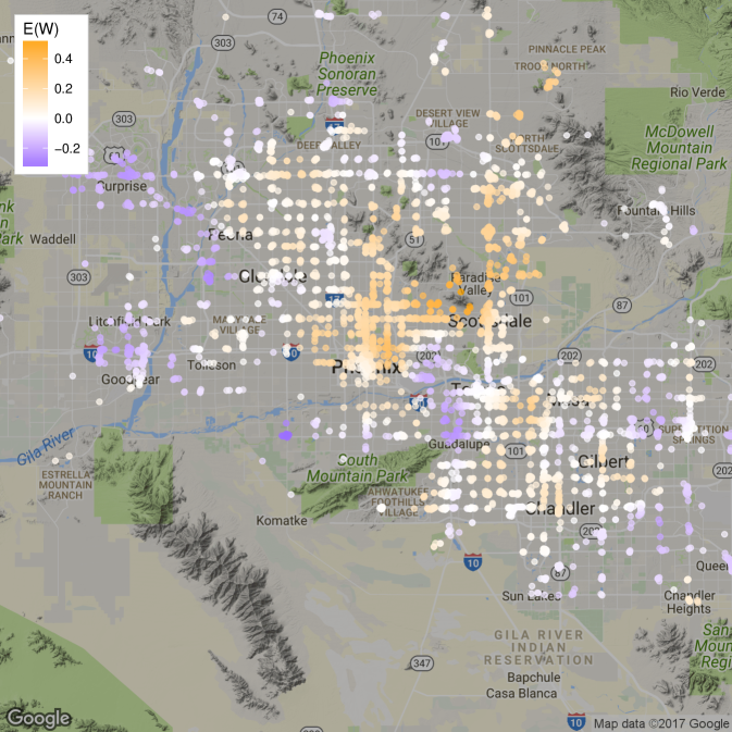
Figure 5 displays the learned spatial field where is the posterior mean of . The results suggest that the downtown Phoenix business district and the area surrounding the affluent Paradise Valley possesses a higher concentration of highly-rated restaurants than the rest of the Phoenix area. More sparsely populated areas such as such as Litchfield Park, or areas with lower income such as Guadalupe, seem to have fewer highly-rated restaurants.
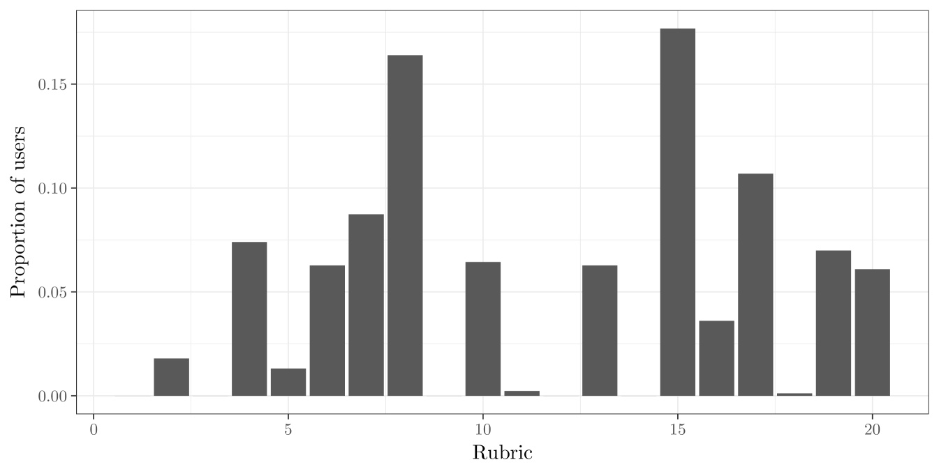
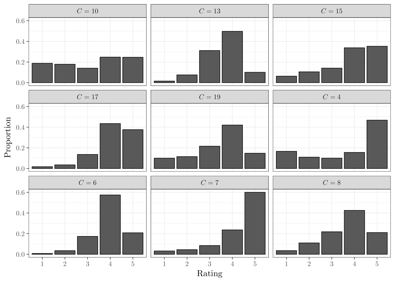
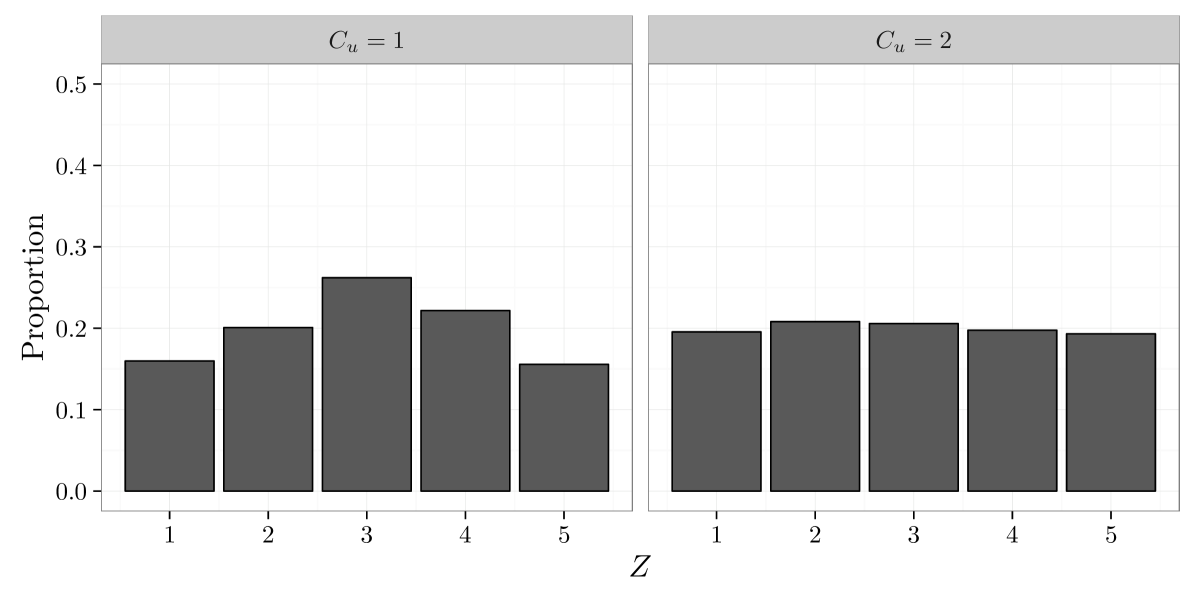
We now examine the individual rubrics. First, we obtain a clustering of users into their rubrics by minimizing Binder’s loss function (Binder,, 1978) , where is the Kronecker delta, is an assignment of users to rubrics, and is the posterior probability of . See Fritsch and Ickstadt, (2009) for additional approaches to clustering objects using samples of the ’s.
The multi-rubric model produces interesting effects on the overall estimate of restaurant quality. Consider the rubric corresponding to in Figure 7. Users assigned to this rubric give the majority of restaurants a rating of five stars. As a result, a rating of 5 stars for the rubric is less valuable to a restaurant than a rating of 5 stars from a user with the rubric. Similarly, a rating of stars from the rubric is more damaging to the estimate of a restaurant’s quality than a rating of stars from the rubric.
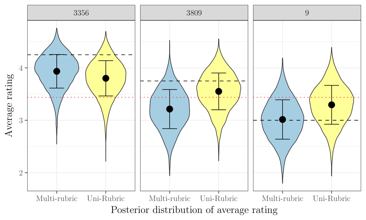
For restaurants with a large number of reviews, the effect mentioned above is negligible, as the restaurants typically have a good mix of users from different rubrics. The effect on restaurants with a small number of reviews, however, can be much more pronounced. To illustrate this effect, Figure 8 displays the posterior distribution of the quantity defined in (2) for the restaurants with . Each of these businesses has reviews total, with empirically averaged ratings of 4.25, 3.75, and 3 stars. For and , the users are predominantly from the rubric with ; as a consequence, the fact that these restaurants do not have an average rating closer to five stars is quite damaging to the estimate of the restaurant quality. In the case of , the effect is strong enough that what was ostensibly an above-average restaurant is actually estimated to be below average by the multi-rubric model. Conversely, item has ratings of , and stars, but one of the -star ratings comes from a user assigned to the rubric which gave a -star rating to only 8% of businesses. As a result, the -star ratings are weighted more heavily than they would otherwise be, causing the distribution of to be shifted slightly upwards.
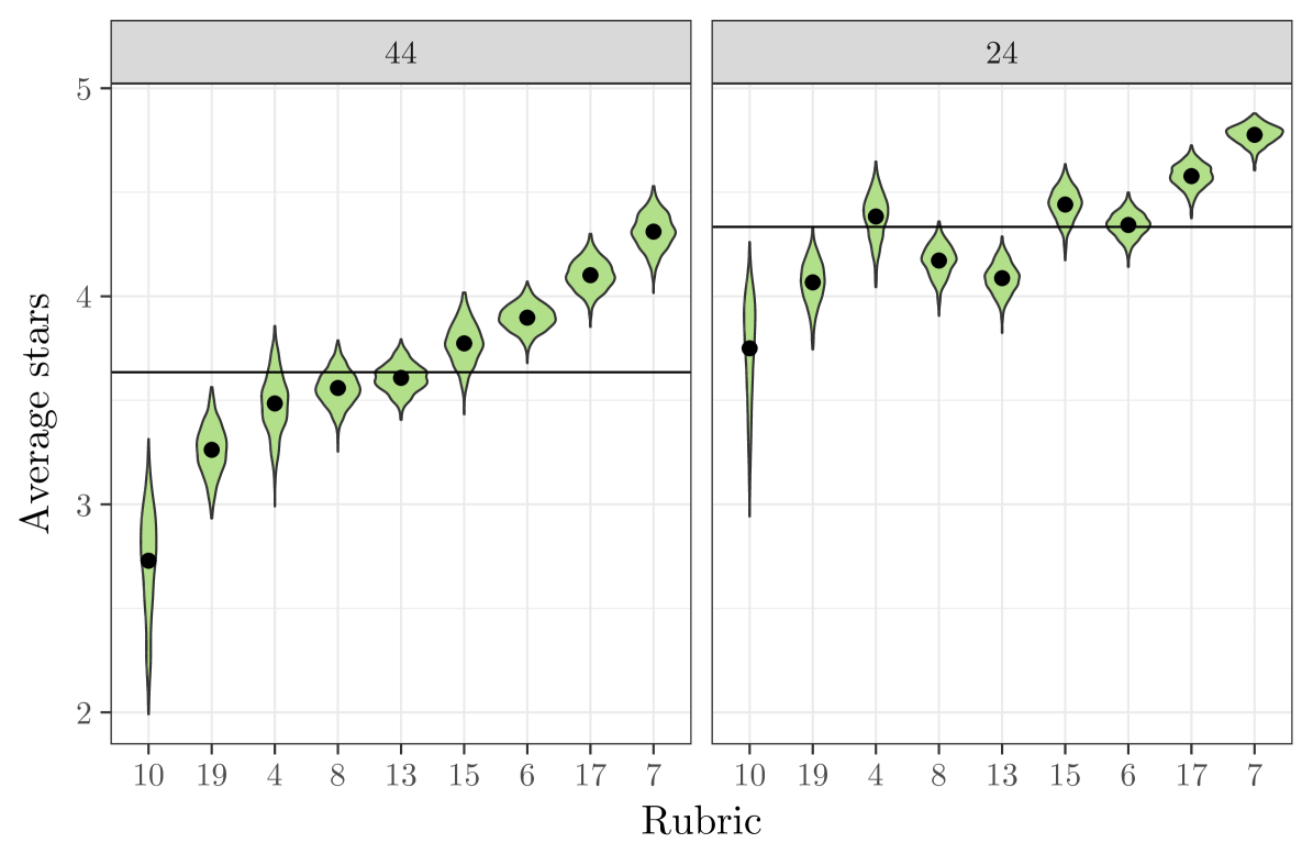
Lastly, we consider rescaling the average ratings according to a specific rubric. This may of interest, for example, if one is interested in standardizing the ratings to match a rubric which evenly disperses ratings evenly across the possible stars. To do this, we examine the rubric-adjusted average ratings given by (3). Figure 9 displays the posterior density of for and , for the most common rubrics. These two restaurants have over 100 reviews, and so the overall quality can be estimated accurately. We see some expected features; for example, the quality of each restaurant has been adjusted downwards for users of the rubric, and upwards for the rubric. The multi-rubric model allows for more nuanced behavior of the adjusted ratings than simple upward/downward shifts. For example, for the mediocre item , we see that little adjustment is made for the rubric, while for the high-quality item a substantial downward adjustment is made. This occurs because the model interprets the users with as requiring a relatively large amount of utility to rate an item 5 stars, so that a downward adjustment is made for the high-quality item; on the other hand, users with tend to rate things near a , so little adjustment needs to be made for the mediocre item.
5 Discussion
In this paper we introduced the multi-rubric model for the analysis of rating data and applied it to public data from the website Yelp!. We found that the multi-rubric model yields improved predictions and induces sophisticated shrinkage effects on the estimated quality of the items. We also showed how the model developed can be used to partition the users into interpretable latent classes.
There are several areas exciting areas for future work. First, while Markov chain Monte Carlo works well for the Yelp! dataset (it took 90 minutes to fit the model of Section 4), it would be desirable to develop a more scalable procedure, such as stochastic variational inference (Hoffman et al.,, 2013). Second, the model described here features limited modeling of the users. Information regarding which items the users have rated has been shown in other settings to improve predictive performance; temporal heterogeneity may also be present in users.
The latent class model described here can also be extended to allow for more flexible models for the ’s and ’s. For example, a referee pointed out the possibility of inferring about how controversial an item is across latent classes, which could be accomplished naturally by using a mixture model for the ’s.
A fruitful area for future research is the development of methodology for when MAR fails. One possibility for future work is to extend the model to also model the missing data indicators . This is complicated by the fact that, while is not completely observed, is. As a result, the data becomes much larger when modeling the ’s.
Acknowledgements
The authors thank Eric Chicken for helpful discussions. This work was partially supported by the Office of the Secretary of Defense under research program #SOT-FSU-FATs-06 and NSF grants NSF-SES #1132031 and NSF-DMS #1712870.
Appendix A Markov chain Monte Carlo algorithm
Before describing the algorithm, we define several quantities. First, define
Let Then we can write
where has rows composed of ’s associated to users who rated item , has rows composed of ’s associated to items which were rated by user , and and are design matrices associated to the covariates and basis functions respectively. Holding the other parameters fixed, each term above on the left-hand-side is sufficient for its associated parameter on the right-hand-side.
A data augmentation strategy similar to the one proposed by Albert and Chib, (1997) is employed. The updates for the parameters , and use a back-fitting strategy based on the ’s above. The Markov chain operates on the state space . We perform the following updates for each iteration of the sampling algorithm, where each step is understood to be done for each relevant and .
-
1.
Draw where is proportional to
-
2.
Draw , for .
-
3.
Draw where and .
-
4.
Draw where and .
-
5.
Draw where and .
-
6.
Draw where and .
-
7.
Draw where and .
-
8.
Draw where .
-
9.
Make an update to which leaves invariant.
-
10.
Make an update to which leaves invariant.
-
11.
Make an update to which leaves invariant.
-
12.
Make an update to which leaves invariant.
In our illustrations, we use slice sampling (Neal,, 2003) to do updates 9–11. The chain is initialized by simulation from the prior with . The only non-trivial step is constructing an update for the ’s. We use a modification of the approach outlined in Albert and Chib, (1997), which uses a Laplace approximation to construct a proposal for the full-conditional of the parameters and for . To alleviate computational burden, the proposal is updated every iteration.
References
- Albert and Chib, (1997) Albert, J. and Chib, S. (1997). Bayesian methods for cumulative, sequential and two-step ordinal data regression models. Technical report, Department of Mathematics and Statistics, Bowling Green State University, Bowling Green, OH.
- Albert and Chib, (1993) Albert, J. H. and Chib, S. (1993). Bayesian analysis of binary and polychotomous response data. Journal of the American Statistical Association, 88:669–679.
- Banerjee et al., (2008) Banerjee, S., Gelfand, A. E., Finley, A. O., and Sang, H. (2008). Gaussian predictive process models for large spatial data sets. Journal of the Royal Statistical Society, Series B, 70:825–848.
- Bao and Hanson, (2015) Bao, J. and Hanson, T. E. (2015). Bayesian nonparametric multivariate ordinal regression. Canadian Journal of Statistics, 43(3):337–357.
- Berret and Calder, (2012) Berret, C. and Calder, C. A. (2012). Data augmentation strategies for the Bayesian spatial probit regression model. Computational Statistics & Data Analysis, 56:478–490.
- Binder, (1978) Binder, D. A. (1978). Bayesian cluster analysis. Biometrika, 65(1):31–38.
- Bobadilla et al., (2013) Bobadilla, J., Ortega, F., Hernando, A., and Gutiérrez, A. (2013). Recommender systems survey. Knowledge-Based Systems, 46:109–132.
- Bradley et al., (2015) Bradley, J. R., Holan, S. H., and Wikle, C. K. (2015). Multivariate spatio-temporal models for high-dimensional areal data with application to longitudinal employer-household dynamics. Annals of Applied Statistics, 9:1761–1791.
- Bradley et al., (2016) Bradley, J. R., Wikle, C. K., and Holan, S. H. (2016). Bayesian spatial change of support for count-valued survey data with application to the american community survey. Journal of the American Statistical Association, 111:472–487.
- Cargnoni et al., (1997) Cargnoni, C., Müller, P., and West, M. (1997). Bayesian forecasting of multinomial time series through conditionally Gaussian dynamic models. Journal of the American Statistical Association, 92:640–647.
- Carlin and Polson, (1992) Carlin, B. P. and Polson, N. G. (1992). Monte Carlo Bayesian methods for discrete regression models and categorical time series. In Bernardo, J. M., Berger, J. O., Dawid, A. P., and Smith, A., editors, Bayesian Statistics 4. Oxford, UK: Oxford Univ. Press.
- Chen and Dey, (2000) Chen, M. H. and Dey, D. K. (2000). A unified Bayesian approach for analysing correlated ordinal response data. Brazilian Journal of Probability and Statistics, 14:87–111.
- Cowles, (1996) Cowles, M. K. (1996). Accelerating Monte Carlo Markov chain convergence for cumulative-link generalized linear models. Statistics and Computing, 6(2):101–111.
- Cressie, (2015) Cressie, N. (2015). Statistics for Spatial Data. John Wiley & Sons, New York, NY.
- Cressie and Johannesson, (2008) Cressie, N. and Johannesson, G. (2008). Fixed rank kriging for very large spatial data sets. Journal of the Royal Statistical Society, Series B, 70:209–226.
- De Oliveira, (2000) De Oliveira, V. (2000). Bayesian prediction of clipped Gaussian random fields. Computational Statistics & Data Analysis, 34(3):299–314.
- De Oliveira, (2004) De Oliveira, V. (2004). A simple model for spatial rainfall fields. Stochastic Environmental Research and Risk Assessment, 18(2):131–140.
- DeYoreo and Kottas, (2014) DeYoreo, M. and Kottas, A. (2014). Bayesian nonparametric modeling for multivariate ordinal regression. arXiv preprint arXiv:1408.1027.
- Escobar and West, (1995) Escobar, M. D. and West, M. (1995). Bayesian density estimation and inference using mixtures. Journal of the American Statistical Association, 90:577–588.
- Ferguson, (1973) Ferguson, T. S. (1973). A Bayesian analysis of some nonparametric problems. The Annals of Statistics, 1:209–230.
- Fritsch and Ickstadt, (2009) Fritsch, A. and Ickstadt, K. (2009). Improved criteria for clustering based on the posterior similarity matrix. Bayesian Analysis, 4(2):367–391.
- Gelman et al., (2006) Gelman, A. et al. (2006). Prior distributions for variance parameters in hierarchical models. Bayesian Analysis, 1(3):515–534.
- Gill and Casella, (2009) Gill, J. and Casella, G. (2009). Nonparametric priors for ordinal Bayesian social science models: Specification and estimation. Journal of the American Statistical Association, 104(486):453–454.
- Härdle and Müller, (2000) Härdle, W. and Müller, M. (2000). Multivariate and semiparametric kernel regression. In Schimek, M., editor, Smoothing and Regression: Approaches, Computation, and Application. New York: John Wiley & Sons, Inc.
- Higgs and Hoeting, (2010) Higgs, M. D. and Hoeting, J. A. (2010). A clipped latent variable model for spatially correlated ordered categorical data. Computational Statistics & Data Analysis, 54:1999–2011.
- Hoffman et al., (2013) Hoffman, M. D., Blei, D. M., Wang, C., and Paisley, J. W. (2013). Stochastic variational inference. Journal of Machine Learning Research, 14(1):1303–1347.
- Houlsby et al., (2014) Houlsby, N., Hernández-Lobato, J. M., and Ghahramani, Z. (2014). Cold-start active learning with robust ordinal matrix factorization. In International Conference on Machine Learning, pages 766–774.
- Ishwaran and Zarepour, (2002) Ishwaran, H. and Zarepour, M. (2002). Dirichlet prior sieves in finite normal mixtures. Statistica Sinica, 12:941–963.
- Knorr-Held, (1995) Knorr-Held, L. (1995). Dynamic cumulative probit models for ordinal panel-data; a Bayesian analysis by Gibbs sampling. Technical report, Ludwig-Maximilians-Universitat.
- Koren and Sill, (2011) Koren, Y. and Sill, J. (2011). OrdRec: an ordinal model for predicting personalized item rating distributions. In Proceedings of the fifth ACM conference on Recommender systems, pages 117–124. ACM.
- Kottas et al., (2005) Kottas, A., Müller, P., and Quintana, F. (2005). Nonparametric Bayesian modeling for multivariate ordinal data. Journal of Computational and Graphical Statistics, 14(3):610–625.
- Linero, (2016) Linero, A. R. (2016). Bayesian regression trees for high dimensional prediction and variable selection. Journal of the American Statistical Association. To appear.
- Marlin and Zemel, (2009) Marlin, B. M. and Zemel, R. S. (2009). Collaborative prediction and ranking with non-random missing data. In Proceedings of the third ACM conference on Recommender systems, pages 5–12. ACM.
- Neal, (2003) Neal, R. M. (2003). Slice sampling. The Annals of Statistics, 31:705–767.
- Paquet et al., (2012) Paquet, U., Thomson, B., and Winther, O. (2012). A hierarchical model for ordinal matrix factorization. Statistics and Computing, 22(4):945–957.
- Rasmussen and Williams, (2005) Rasmussen, C. E. and Williams, C. K. I. (2005). Gaussian Processes for Machine Learning (Adaptive Computation and Machine Learning). The MIT Press, Cambridge, MA.
- Salakhutdinov and Mnih, (2007) Salakhutdinov, R. and Mnih, A. (2007). Probabilistic matrix factorization. In Advances in Neural Information Processing Systems, pages 1257–1264.
- Sang and Huang, (2012) Sang, H. and Huang, J. Z. (2012). A full scale approximation of covariance functions for large spatial data sets. Journal of the Royal Statistical Society: Series B (Statistical Methodology), 74(1):111–132.
- Schliep and Hoeting, (2015) Schliep, E. M. and Hoeting, J. A. (2015). Data augmentation and parameter expansion for independent or spatially correlated ordinal data. Computational Statistics & Data Analysis, 90:1–14.
- Simpson et al., (2017) Simpson, D., Rue, H., Riebler, A., Martins, T. G., Sørbye, S. H., et al. (2017). Penalising model component complexity: A principled, practical approach to constructing priors. Statistical Science, 32(1):1–28.
- Teh et al., (2006) Teh, Y. W., Jordan, M. I., Beal, M. J., and Blei, D. M. (2006). Hierarchical Dirichlet processes. Journal of the American Statistical Association, 101(476):1566–1581.
- Velozo et al., (2014) Velozo, P. L., Alves, M. B., and Schmidt, A. M. (2014). Modelling categorized levels of precipitation. Brazilian Journal of Probability and Statistics, 28:190–208.
Supplementary Material Antonio R. Linero, Jonathan R. Bradley, Apruva S. Desai
Appendix S.1 Identifiability
We conduct a brief simulation experiment to illustrate that model proposed in Section 2.3 is capable of (i) identifying the correct number of latent factors and (ii) capable of accruing evidence about the individual ’s and ’s. We simulate from the data model, response model, random effect model, spatial process model, and parameter model described in Section 2.3 with the dimension of the latent factor set to . For simplicity, we omit the item-specific covariates given by . For the random effects model we set , and . We set and , with the basis functions given by Gaussian radial basis functions with knots at placed uniformly at random throughout the spatial domain. For the parameter model, we used rubrics with and selected in the manner described in the simulation of Section 3. We set and , and select user/item pairs for inclusion by sampling uniformly at random, with a total of 3981 ratings.
After simulating this data, we fit the multi-rubric model using the correct using the default prior described in Section 2.3 with the correct choice of basis functions , with and .
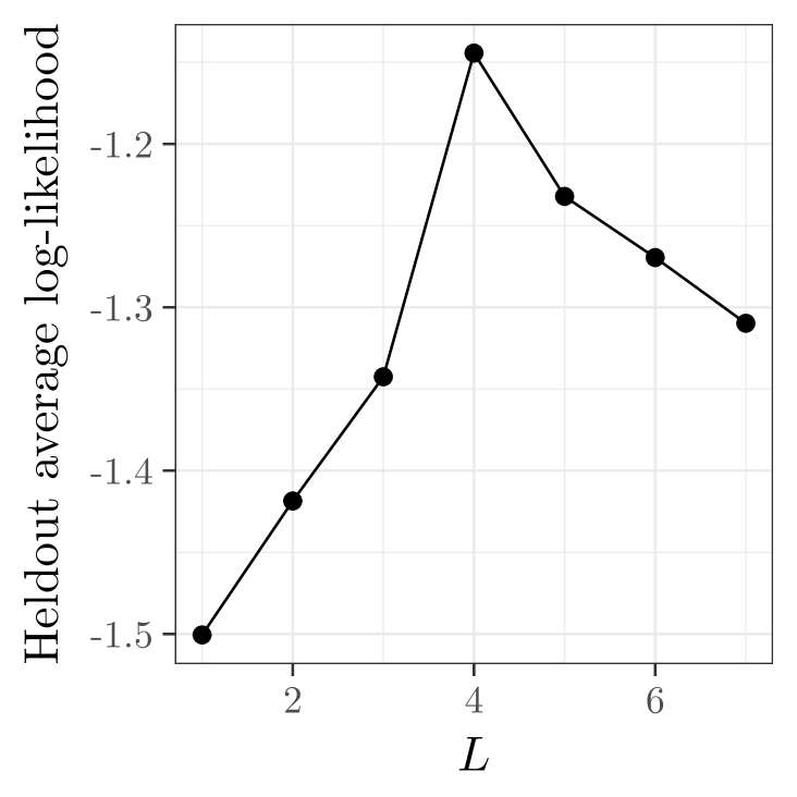
We first assess whether the model is capable of recovering the true number of latent factors. We fit the model for and evaluated each value of by held-out log-likelihood criteria (4) after splitting the data randomly into training and testing sets. Results are given in Figure 10. We see that the model with the highest held-out log-likelihood corresponds to , the correct number of latent factors.
Next, we assess whether the model is capable of learning the individual ’s and ’s. First, we note that for any orthonormal matrix with we have
Moreover, and are equal in distribution (as are and ), so the prior does not provide any additional identification. Consequently, we can only expect to identify and up-to an arbitrary rotation. While it is possible to impose constraints on the and — say, by fixing to know values — this is undesirable because it breaks the symmetry of the prior. In view of this, it is standard in the recommender systems literature to not invoke any constraints on the prior \citepNewsalakhutdinov2007probabilistic.
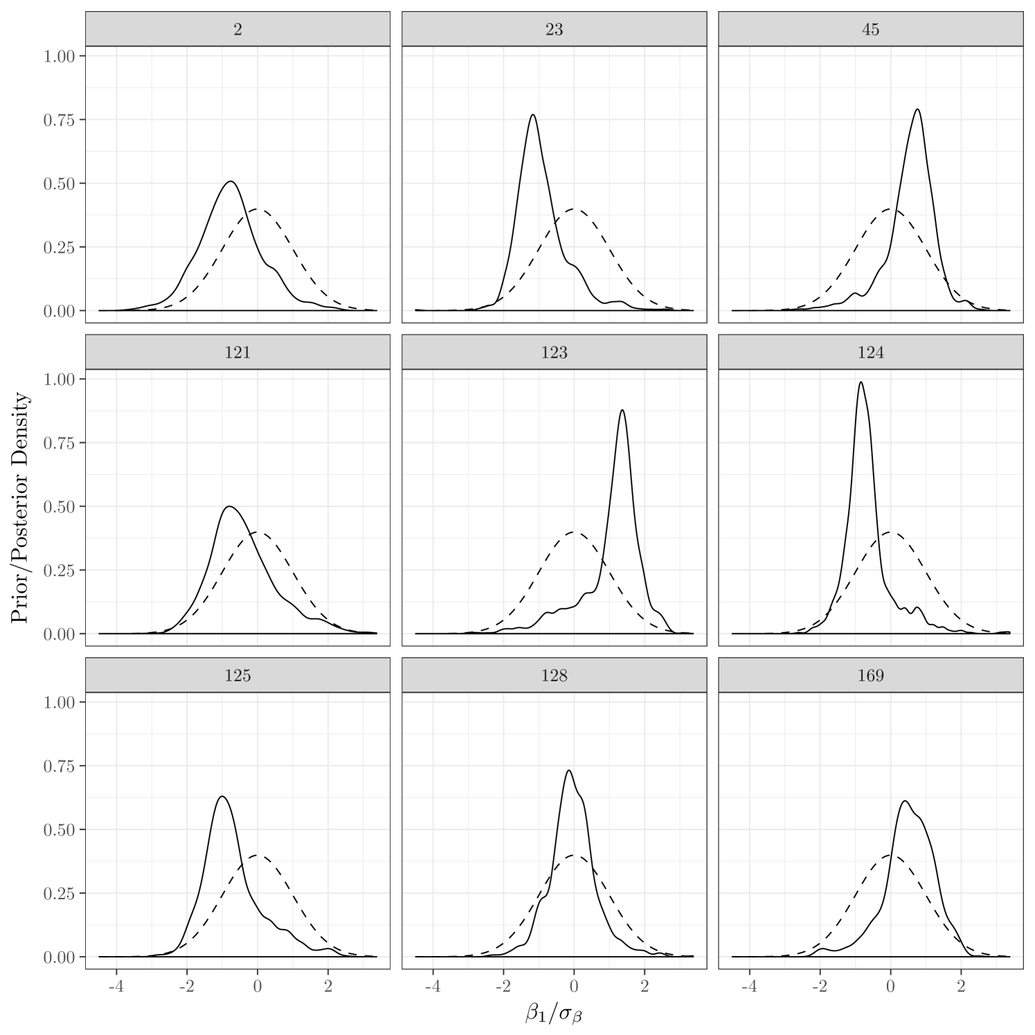
With these points in mind, Figure 11 displays the prior distribution of along with the posterior distribution of ’s for 9 randomly selected items. We see that, while the overall distribution of the ’s is in agreement with the prior when considered as a group, for the individual ’s the prior and posterior differ considerably. This indicates that the model is capable of detecting differences in the ’s across items.
apalike \bibliographyNewmybib.bib