Multi-sine-Gordon Models
Abstract
This work deals with the presence of defect structures in generalized sine-Gordon models. The models are described by periodic potentials, with substructure having one, two, three or more distinct topological sectors, with multiplicity one, two, three or more, respectively. The investigation takes advantage of the deformation procedure introduced in previous work, which is used to introduce the new models, and to study all the defect structures they may comprise.
pacs:
11.27.+d, 11.25.-wI Introduction
In this work we study defect structures in relativistic models described by a single real scalar field, which are of current interest in high energy physics b1 ; b2 and in condensed matter b3 ; b4 . We focus on static solutions in space-time dimensions, with the motivation to present families of models, and the defect structures they may comprise. The models are described by a single real scalar field, engendering discrete symmetry, so we search for defect structures of global nature, known as kinks and lumps.
In high energy physics, kinks and lumps are of interest in several different contexts b1 ; b2 , including supergravity, branes with a single extra dimension and cosmology of branes sugra ; brane ; cbrane ; etc . In condensed matter, they may contribute to pattern formation b3 , and to the description of interfaces among distinct configurations in magnetic systems b4 . They may also appear in other applications, for instance, in the study of nonlinear excitations in Bose-Einstein condensates bec , and in the construction of magnetic apparatus at the nanometric scale a .
We use the deformation procedure introduced in Ref. dd , and we deform the starting model, which is the model engendering spontaneous symmetry breaking, to get to new families of sine-Gordon models. We focus on sine-Gordon models because they are of interest in a diversity of contexts; see, e.g., Refs. sg1 ; sg2 . The procedure is implemented via the deformation function and the parameters it comprises, which leads us to the double and triple sine-Gordon models with analytical solutions, etc. Since the potential of the starting model, the model, can be described by a superpotential which is known explicitly, explicit expressions for the superpotential for deformed models can also be derived, and this leads to important informations on the corresponding BPS states bps , as well as on the energy and stability of the solutions bs of the families of models.
Most of the families of periodic potentials which will be introduced in this work engender periodic substructure, and can be identified by , an integer which describes the multiplicity of the substructure of each potential. In this sense, we will describe a diversity of multi-sine-Gordon models, and the defect structures they may comprise. In particular, the double, triple and other multi-frequency sine-Gordon models are of interest to issues concerning integrability msg , and they can also be used to generate braneworld scenarios with a single extra dimension brane ; cbrane ; etc , with substructures that could appear in the form of multi-brane scenarios. The scalar field used to describe the periodic models could also interact with another scalar field, to give rise to defect inside defect did , and to allow for the presence of brane with internal structure bis . In this sense, the present work provides a variety of multi-sine-Gordon models, and study the presence of topological structure at the classical level, offering results which are of current interest to high energy physics, and to other areas of nonlinear science.
We organize the work as follows: In the next Sect. II we describe the main steps of the deformation procedure. In Sect. III we single out the deformation function which will be used throughout the work, and there we study specific sine-Gordon models. In Sect. IV we introduce the superpotentials corresponding to the multi sine-Gordon models studied in the previous Sect. III, and we calculate the energies corresponding to several specific solutions the models comprise. Finally, in Sect. V we present comments and conclusions.
II The procedure
We start the investigation with a quick review of the deformation procedure dd . We consider two real scalar fields and and the corresponding models, described by the Lagrange densities,
| (1a) | |||
| (1b) | |||
Here, and are given potentials, which specify each one of the two models. We introduce a function named deformation function, from which we link the model (1a) with the deformed model (1b) by relating the two potentials and in the very specific form
| (2) |
where means that in the potential , we change by . In this case, if the starting model has finite energy static solution which obeys the equation of motion
| (3) |
then the deformed model may also have finite energy static solution given by
| (4) |
which obeys
| (5) |
We note that if the deformation function has critical points, the deformation procedure works smoothly if and only if the potential has zeros of multiplicity at least two at those critical points. The critical points of are the branching points of which is consequently a multivalued function.
The deformation procedure has been used by several authors in a diversity of scenarios, and it appears to work correctly in many distinct situations ddsal ; dd+ .
We go further into the problem using the standard model
| (6) |
This is the model, with spontaneous symmetry breaking. Here we are using natural units, and we have rescaled the field, and the space and time coordinates to make them dimensionless. This model has as topological defects the BPS states , and we choose the center of the solutions at the origin , for simplicity. The energy density is given by , which gives the energy . We also note that the potential has minima at and obeys: , and , where , etc. Next, if we choose the deformation function in the form , we get to the potential
| (7) |
In this case the deformation function depends only on , and the corresponding deformed model describes the sine-Gordon model, with no extra parameter involved in the procedure. This model has solutions described by
| (8) |
where identifies the particular topological sector of the sine-Gordon model, which has an infinity of sectors. We then see that we go from the model, which contains a single topological sector, to the sine-Gordon model, which contains an infinity of topological sectors, by the use of the deformation , which is a periodic function, which needs the presence of the integer to identify the particular periodic sector, which is naturally used to identify the particular topological sector of the deformed model, as we have just shown.
III New families of models
Here we follow the methodology of Ref. ddsal , searching for new functions , from which we can build families of periodic models. We take the starting model described by the potential (6) and the kink-like solution , and we choose the deformation function
| (9) |
This function depends on the choice of , on which is real constant, and on , which can be integer or semi-integer: for integer, the deformed potential can be written in the form
| (10) |
where . If we choose semi-integer, we get
| (11) |
As we show below, using integer values for the parameter lead the number of vacua of the new model to be fixed at will.
The choice (9) is a generalization of the deformation function used in ddsal . There, the deformation function was taken as , and this allowed to generate families of polynomial potentials. In the present work, below we will take as a periodic function of the scalar field, and this will generate new families of models, with periodic potentials, as generalized sine-Gordon potentials. All the potentials are new periodic potentials, and we solve them finding the defect structures they may comprise directly, using the deformation procedure. In this sense, the present work contribute to offer new models, to study the defect structures they may comprise, and to strengthen the power of the deformation procedure introduced in dd .
In general, the above models identify families of potentials which present static solutions given by
| (12) |
where represents the inverse of . Also, , with . However, to investigate specific models, let us start with (10) and . Here the potentials are, for odd,
| (13) |
and for even,
| (14) |
where .
Here we see that the choice leads us to polynomial potentials, as already investigated in Ref. ddsal . In the present work, however, we want to study periodic potentials, of the sine-Gordon type. For this reason, we consider as a periodic function of the scalar field. If we take , from (10) and (11), we have the potentials
| (17) |
and
| (18) |
which are sine-Gordon potentials with multiplicity , with the parameter now controlling the amplitude and periodicity of the potential. In order to obtain new sine-Gordon potentials with higher multiplicity, in the next subsections we take the function , where will be chosen appropriately.
III.1 New sine family of models
Let us now consider the function , where is integer and is one of the zeros of the potentials (13), and (14), except , and . In this case, we have with , for even, and , for odd.
The polynomial form of , with its zeros (and multiplicities), for , are known ddsal . Thus, performing the deformation in Eqs. (13) and (14), we have:
-
•
for odd:
(19) -
•
for even:
(20)
where . The potential can be written in terms of the Chebyshev polynomials of second kind:
| (21a) | |||
| (21b) |
The explicit forms of , for and are given by
| (22) | |||||
| (23) | |||||
which illustrate the new family of models.
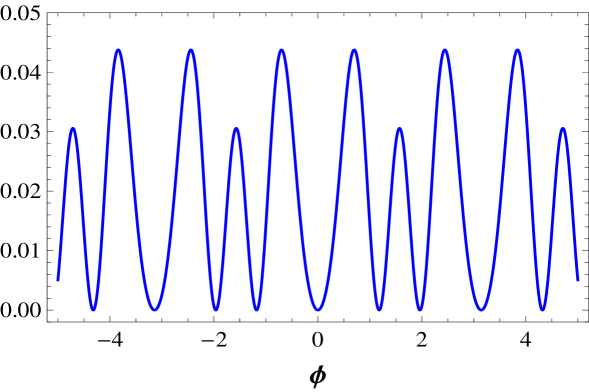
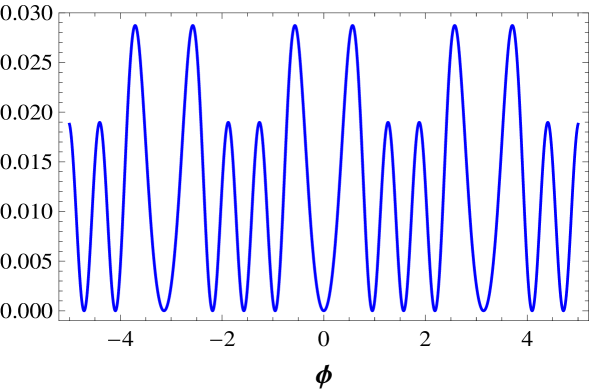
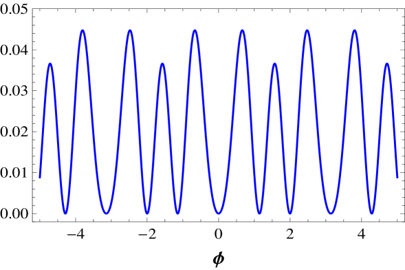
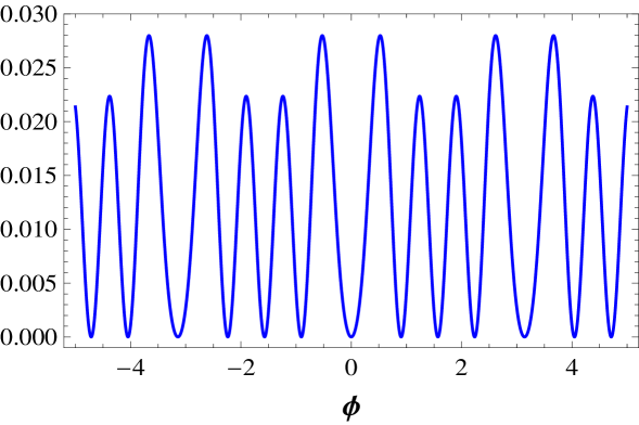
We note that we have a diversity of sine-Gordon models, which includes variations of the sine-Gordon model, and the double sine-Gordon, triple sine-Gordon, and so on. We illustrate these models depicting in Fig. 1 the potentials and , and in Fig. 2, the potentials and .
III.1.1 Static solutions
An important advantage of the use of the deformation procedure is that it gives the defect structures explicitly. From (12) and , in the case above, we have the static solutions of the given by
| (26) |
where , and is integer in the range: .
III.1.2 Maxima and minima
The maxima and minima of the potentials appear when we take the derivative of these potentials with respect to the field to be zero. If the potential is non negative, then the minima are also zeros of it. These informations help us a lot, and in the case of the above potentials, , we can write, for odd, the minima
| (27) |
and
| (28) |
where . The maxima are
| (29) |
and , which obeys
| (30) |
The maxima (29) have the height, , and the height of the others maxima comes from Eq. (30), which can be solved numerically. In the table below we show some examples, for several values of and . We recall that the maxima are periodic, so in the table we show some positive ones, closer to zero, which represent families of maxima.
| - | - | - | |||||||
| - | - | - | |||||||
| - | - | - | - | - | |||||
| - | - | - | - | - | |||||
| - | - | - | - | - | - | - | |||
| - | - | - | - | - | - | - | |||
| - | - | - | - | - | - | - | - | ||
| - | - | - | - | - | - | - | - |
III.2 New cosine family of models
Here, we consider the function , where is integer and is one of the zeros of the potentials (15), and (16), except and . In the case of the family, we have , with , for even, and , for odd.
The polynomial form of , with its zeros (and multiplicities), for , are known ddsal . Thus, we apply the deformation in Eqs. (15) and (16) to get:
-
•
for odd:
(31) -
•
for even:
(32)
where . The potentials are given by Chebyshev polynomials, of the first kind:
| (33a) | |||
| (33b) |
The explicit form of , for and with are given by
which illustrate this new family of models. Here we note that, we have a diversity of sine-Gordon models, which includes variations of the sine-Gordon model, and the double sine-Gordon, triple sine-Gordon, and so on.
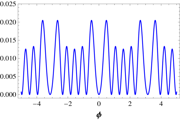
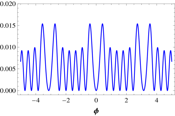
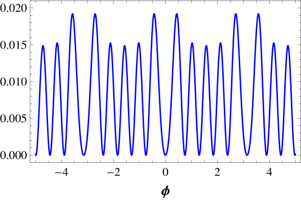
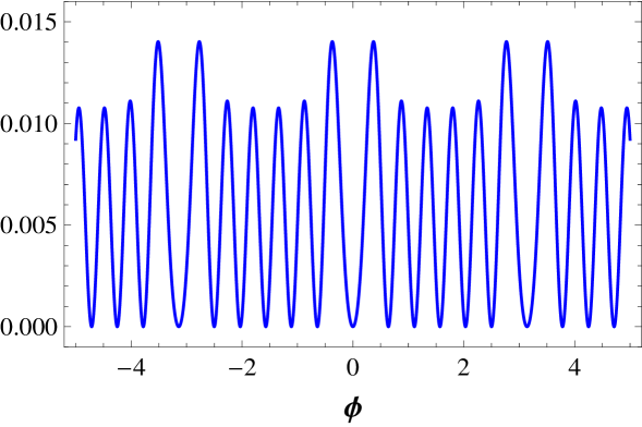
We illustrate some potentials in Fig. 3, where we plot and and in Fig. 4, where we plot and .
III.2.1 Static solutions
We use (12) and to get the static solutions of the family of models. Here we have
| (36) |
where , and is integer such that .
III.2.2 Maxima and minima
Again, like in the case of the family, the above potentials are non negative. Therefore, the minima are calculated taking , and from the derivative of the potential, excluding the minima, we obtain the maxima. For odd, the minima are
| (37) |
and
| (38) |
where . And, the maxima came from the equation
| (39) |
where , which can be solved numerically, as we did before, for the previous family of models.
III.3 Kink Multiplicity
The potential of the sine-Gordon model has an infinity of topological sectors, and supports essencially the same kind of kink. Thus, if denotes the kink multiplicity, as already informed, then for the sine-Gordon model the kink multiplicity is . In the double sine-Gordon model we have two distinct topological sectors, so the kink multiplicity is , for the double sine-Gordon model. For the triple sine-Gordon model model we have three distinct topological sectors, so the kink multiplicity is , and so on. For the periodic models introduced above, we have been able to write the kink multiplicity in terms of the parameter , and in the table below, we summarize the kink multiplicity corresponding to each member of the and family of potentials for integer.
| Family | odd | even |
|---|---|---|
We note that the kink multiplicity depends directly on , so it increases when also increases.
IV Superpotentials and energies
It is sometimes possible to derive explicit expressions for superpotentials. If is a function of the scalar field, it is the superpotential if the potential is written in the form
| (40) |
where the prime stands for the derivative with respect to the field. Now, from the deformation procedure we can write that if is the superpotential of the starting model, then the superpotential of the deformed model has to obey
| (41) |
In the case of the model which we are using to implement the deformation procedure, we have
| (42) |
and this can be used to get to the superpotentials of the deformed models.
The expressions of the superpotentials are of great use, since they can be used to get the energies of the corresponding defect structures, since we know that the energy of a topological defect with the potential described by the superpotential is given by
| (43) |
where , for being the static kinklike solution.
Alternatively, the superpotential can be directly obtained from the integration of Eq. (40),
| (44) |
but the integral does not in general lead to an explicit formula for . However, this is not the case here, and the explicit form of the superpotentials corresponding to the family, for and are given by
| (45) |
| (46) |
| (47) |
| (48) |
| (49) |
| (50) |
For the family, the explicit form of the superpotentials for are given by
| (51) | |||||
| (52) | |||||
The above expressions allow us to get the energy corresponding to each distinct topological sector. To illustrate this issue, let us calculate some energies. We start with the family of models. The potential has multiplicity , so it has only one kind of kink, with energy . The potential has multiplicity , and the kink has energy . The potential which is plotted in Fig. 1 has multiplicity , so it has two distinct kinks, which we name large and small kinks, the large one representing the kink in the sector where the maxima of the potential has higher height; here the kink energies are given by and . The potential is plotted in Fig. 1, and it also has multiplicity ; here the corresponding energies are and . Another potential is , which is plotted in Fig. 3. It has multiplicity , and the corresponding kink energies are , , and , for the large, medium, and small kink, respectively.
Let us now deal with the family of models. The potential has multiplicity . The kink energy is . The potential also has multiplicity , and the kink energy is . The potential is shown in Fig. 3, and it has multiplicity . Here the two kink energy are and , for large and small kink, respectively. The potential is plotted in Fig. 3, and it also has multiplicity . The kink energies are and . Another potential is , which is depicted in Fig. 4. It has multiplicity , and the corresponding kink energies are , , and , for large, medium, and small kink, respectively.
V Final comments
In this work we studied a diversity of models described by periodic potentials. The investigation makes use of the deformation procedure, which allows to get to new families of periodic potentials, and to explore all the topological sectors and the corresponding defect structures they may comprise. The periodic potentials present a multiplicity of distinct topological sectors, which we used to define the multi-sine-Gordon models.
It is worth emphasizing that we have obtained the superpotentials explicitly, which is important to investigate the kink energies. Also, the kink solutions for all the models are known explicitly. In this sense, we believe it is of current interest to investigate how the study of Ref. sg2 works for the above families of models, and how the results of Ref. msg can be used to the new models introduced in this paper.
The present work opens new lines of investigations. An interesting issue concerns the problem of using the above multi-sine-Gordon models to introduce new braneworld scenarios, in which the brane can engender multistructure. This investigation can be done under the lines of brane ; etc ; bis . These and other related issues are under consideration, and we hope to report on them in the near future.
Acknowledgements.
The authors would like to thank CAPES, CNPq, and the Nanobiotec/CAPES program, for partial financial support.References
- (1) A. Vilenkim and E.P.S. Shellard, Cosmic strings and other topological defects (Cambridge, Cambridge/UK, 1994).
- (2) N. Manton and P. Sutcliffe, Topological solitons (Cambridge, Cambridge/UK, 2004).
- (3) D. Walgraef, Spatio-temporal pattern formation (Springer-Berlag, New York, 1997).
- (4) G. Bertotti, Hysteresis in magnetism (Academic, San Diego/CA, 1998).
- (5) M. Cvetic and H.H. Soleng, Phys. Rep. 282, 159 (1997).
- (6) L. Randall and R. Sundrum, Phys. Rev. Lett. 83, 3370 (1999); Phys. Rev. Lett. 83, 4690 (1999); W.D. Goldberger and M.B. Wise, Phys. Rev. Lett. 83, 4922 (1999); O. DeWolfe, D.Z. Freedman, S.S. Gubser, and A. Karch, Phys. Rev. D 62, 046008 (2000); C. Csáki, J. Erlich, T.J. Hollowood, and Y. Shirman, Nucl. Phys. B 581, 309 (2000).
- (7) G. Dvali, G. Gabadadze, and M. Porrati, Phys. Lett. B 485, 208 (2000); G. Dvali and G. Gabadadze, Phys. Rev. D 63, 065007 (2001); C. Deffayet, Phys. Rev. D 66, 103504 (2002); P. Brax and C. van de Bruck, Class. Quant. Grav. 20, R201 (2003); P. Brax, C. van de Bruck, and A.-C. Davis, Rep. Prog. Phys. 67, 2183 (2004).
- (8) D.Z. Freedman, C. Nunez, M. Schnabl, and K. Skenderis, Phys. Rev. D 69, 104027 (2004); A. Celi et al., Phys. Rev. D 71, 045009 (2005); D. Bazeia, C.B. Gomes, L. Losano, and R. Menezes, Phys. Lett. B 633, 415 (2006); V.I. Afonso, D. Bazeia, and L. Losano, Phys. Lett. B 634, 526 (2006); K. Skenderis and P.K. Townsend, Phys. Rev. Lett. 96, 191301 (2006).
- (9) J. Belmonte-Beitia, V.M. P erez-Garca, V. Vekslerchik, and V.V. Konotop, Phys. Rev. Lett. 100, 164102 (2008); A.T. Avelar, D. Bazeia, and W.B. Cardoso, Phys. Rev. E 79, 025602(R) (2009).
- (10) A. Vanhaverbeke, A. Bischof, and R. Allenspach, Phys. Rev. Lett. 101, 107202 (2008).
- (11) D. Bazeia, L. Losano, and J.M.C. Malbouisson, Phys. Rev. D 66, 101701(R) (2002).
- (12) G. Mussardo, V. Riva, G. Sotkov, Nucl. Phys. B 699, 545 (2004); M. Thies, K. Urlichs, Phys. Rev. D 71, 105008 (2005); H. Blass, H.L. Carrion, JHEP 0701, 027 (2007); D. Bazeia, L. Losano, J. M. C. Malbouisson, R. Menezes, Physica D 237, 937 (2008); L. A. Ferreira, B. Piette, W. J. Zakrzewski, Phys. Rev. E 77, 036613 (2008).
- (13) G. Mussardo, Nucl. Phys. B 779, 101 (2007).
- (14) M.K. Prasad, C.M. Sommerfield, Phys. Rev. Lett. 35, 760 (1975); E.B. Bogomol nyi, Sov. J. Nucl. Phys. 24, 449 (1976).
- (15) D. Bazeia and M.M. Santos, Phys. Lett. A 217, 28 (1996).
- (16) G. Delfino and G. Mussardo, Nucl.Phys. B 516, 675 (1998); G. Z. Tóth, J. Phys. A 37, 9631 (2004); G. Takacs and F. Wagner, Nucl. Phys. B 741, 353 (2006); L. A. Ferreira, W. J. Zakrzewski, The concept of quasi-integrability: a concrete example. arXiv:1011.2176.
- (17) J.R. Morris, Phys. Rev. D 51, 697 (1995). J.D. Edelstein, M.L. Trobo, F.A. Brito, and D. Bazeia, Phys. Rev. D 57, 7561 (1998); D. Bazeia and F. A. Brito, Phys. Rev. D 62,101701(R) (2000); S. M. Carroll, S. Hellerman, and M. Trodden, Phys. Rev. D 61, 065001 (2000).
- (18) A. Campos, Phys. Rev. Lett. 88, 141602 (2002); D. Bazeia, C. Furtado, and A.R. Gomes, JCAP 0402, 002 (2004); D. Bazeia and A.R. Gomes, JHEP 0405, 012 (2004); A. Melfo, N. Pantoja, and J. D. Tempo, Phys. Rev. D 73, 044033 (2006); D. Bazeia, F.A. Brito, L. Losano, JHEP 0611, 064 (2006); V. Dzhunushaliev, Grav. Cosmol. 13, 302 (2007); A. de Souza Dutra, A.C. Amaro de Faria Jr., and M. Hott, Phys. Rev. D 78, 043526 (2008); Yu-Xiao Liu, Li-Da Zhang, Li-Jie Zhang, and Yi-Shi Duan, Phys. Rev. D 78, 065025 (2008); C. A. S. Almeida, M. M. Ferreira Jr., A. R. Gomes, and R. Casana, Phys. Rev. D 79, 125022 (2009); Yu-Xiao Liu, Zhen-Hua Zhao, Shao-Wen Wei, and Yi-Shi Duan, JCAP 02, 003 (2009); Yu-Xiao Liu, Hai-Tao Li, Zhen-Hua Zhao, Jing-Xin Li, and Ji-Rong Ren, JHEP 0910, 091 (2009).
- (19) D. Bazeia, M.A. Gonzalez Leon, L. Losano, J. Mateos Guilarte, Phys. Rev. D 73, 105008 (2006).
- (20) D. Bazeia and L. Losano, Phys. Rev. D 73, 025016 (2006); V.I. Afonso, D. Bazeia, M.A. Gonzalez Leon, L. Losano, J. Mateos Guilarte, Phys. Lett. B 662, 75 (2008); Nucl. Phys. B 810, 427 (2009); A. de Souza Dutra, Physica D 238, 798 (2009); D. Bazeia, L. Losano, R. Menezes, and M.A.M. Sousa, EPL 87, 21001 (2009); W. T. Cruz, M. O. Tahim, and C.A.S. Almeida, EPL 88, 41001 (2009); A.E.R. Chumbes and M.B. Hott, Phys. Rev. D 81, 045008 (2010); D. Bazeia, M.A. Gonzalez Leon, L. Losano, and J. Mateos Guilarte, EPL 93, 21001 (2011).