00 \jnum00 \jyear2013 \jmonthJanuary
Multi-source Pseudo-label Learning of Semantic Segmentation
for the Scene Recognition of Agricultural Mobile Robots
Abstract
This paper describes a novel method of training a semantic segmentation model for scene recognition of agricultural mobile robots exploiting multiple publicly available datasets that are different from the target greenhouse environments. Semantic segmentation models require abundant labels given by tedious manual annotation for training. Although unsupervised domain adaptation (UDA) is studied as a workaround for such a problem, existing UDA methods assume a source dataset similar to the target dataset, which is not available for greenhouse scenes. In this paper, we propose a method to train a semantic segmentation model for greenhouse images leveraging multiple publicly available datasets not dedicated to greenhouses. We exploit segmentation models pre-trained on each source dataset to generate pseudo-labels for the target images based on agreement of all the pre-trained models on each pixel. The proposed method allows for effectively transferring the knowledge from multiple sources rather than relying on a single dataset and realizes precise training of semantic segmentation model. We also introduce existing state-of-the-art methods to suppress the effect of noise in the pseudo-labels to further improve the performance. We demonstrate that our proposed method outperforms existing UDA methods and a supervised SVM-based method.
keywords:
Semantic segmentation, deep Learning, scene recognition, unsupervised domain adaptation (UDA)1 Introduction
Semantic segmentation based on Deep Neural Network (DNN) is widely used in the scene recognition system of self-driving vehicles and autonomous mobile robots. In our research project, we are aiming at developing an agricultural robot that can recognize regions covered by traversable plants and go through them [1, 2]. For such an application, semantic segmentation is suitable since it provides pixel-wise semantic information. Usually, DNNs are trained using a large amount of data with hand-annotated labels to ensure high accuracy and generalization. However, hand-annotation is time consuming and physically demanding. In the case of introducing a mobile robot in new environments, it is not realistic to prepare such a fully labeled dataset for every environment even though a model should be trained specifically for the environment.
To address this problem, one might consider applying a model trained with existing publicly available image datasets with ground truth labels. The performance of pre-trained models, however, often deteriorates on different data domains due to the difference in data distributions between the training dataset and the target scenes, known as “domain shifts” [3]. Domain adaptation (DA) is a task to adapt a model trained on one data domain to another domain with minimal degradation of performance. Unsupervised domain adaptation (UDA) is a type of DA where labeled source datasets and unlabeled target datasets are available. UDA can mitigate the burden of hand-annotation by leveraging information in the source domain and transferring it to the target.
A major task of UDA is adaptation from labeled synthetic images automatically acquired in a simulator to unlabeled real images. The adaptation task from GTA 5 [4] or SYNTHIA [5] to Cityscapes [6] is one of the most widely used benchmarks and many studies have verified their effectiveness on these tasks. However, it is often difficult to prepare appropriate source datasets with full segmentation labels for target environments in the wild. In the case of greenhouses, there is no real image dataset of greenhouses with segmentation labels, and rich simulation environments applicable to our task.
Instead, we consider utilizing publicly available rich image datasets of the real world not specifically designed for greenhouses.
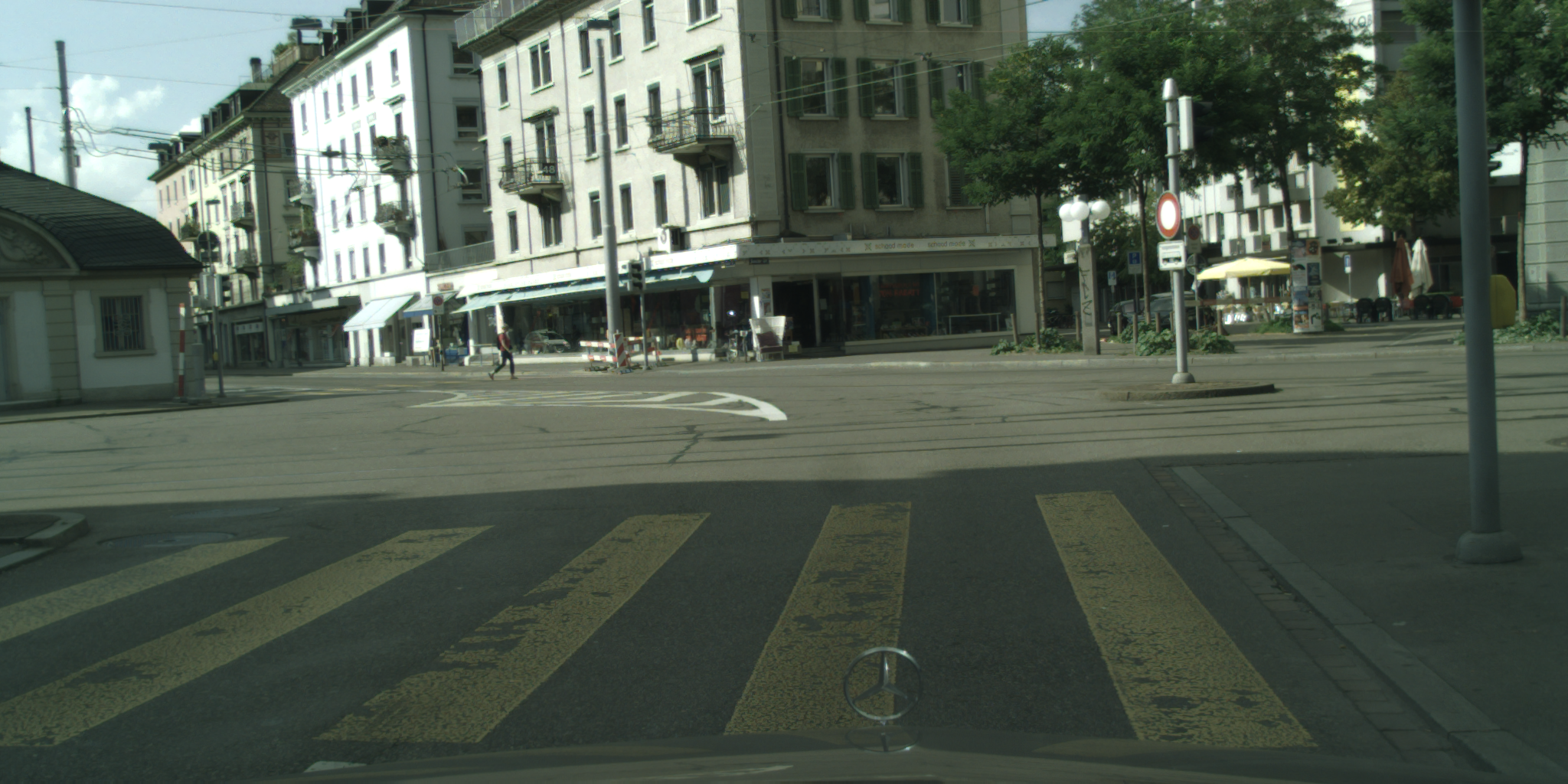
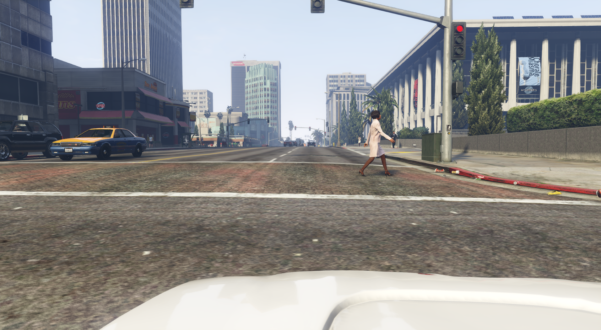
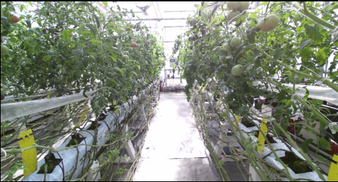
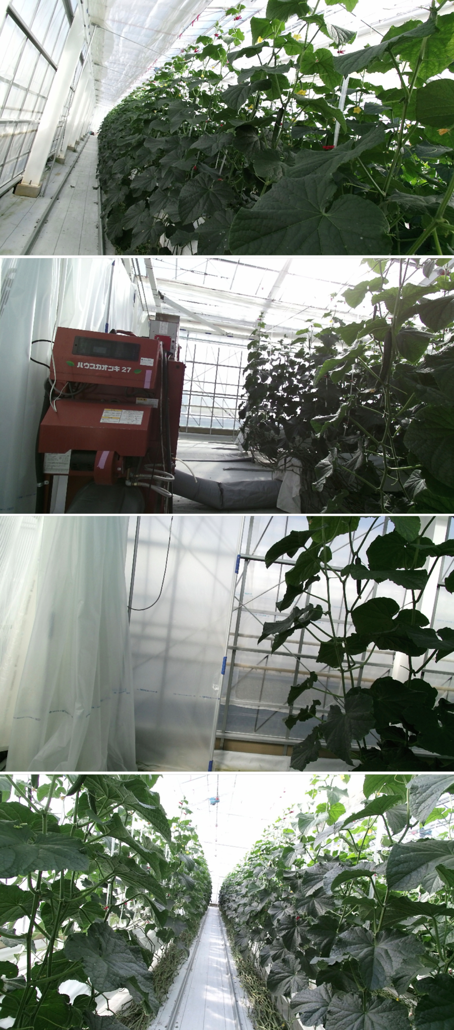
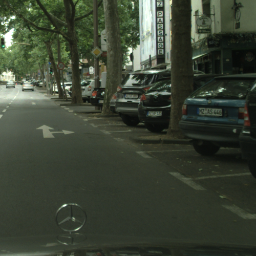
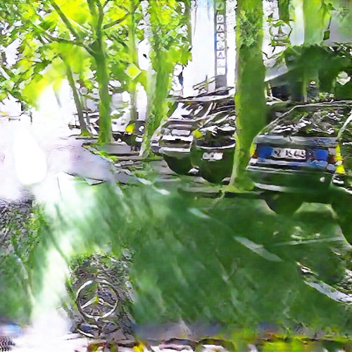
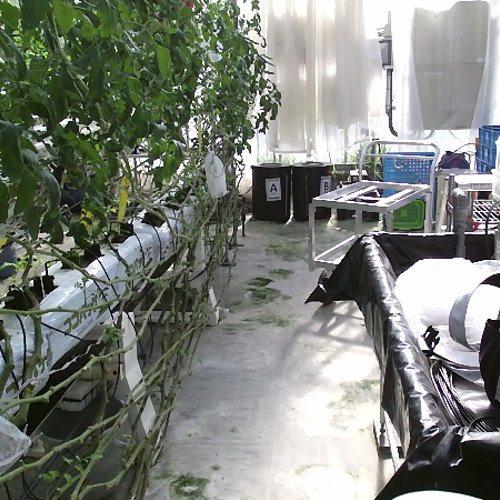
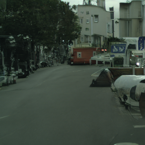
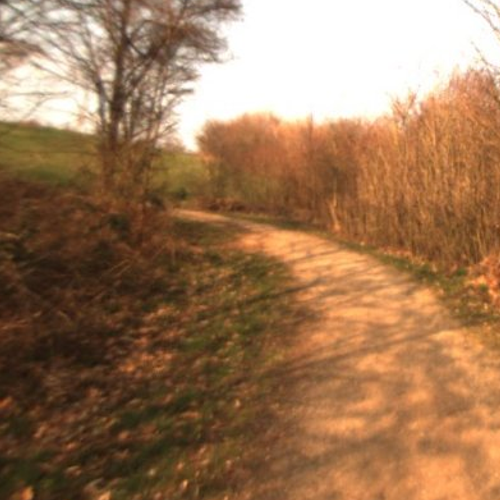
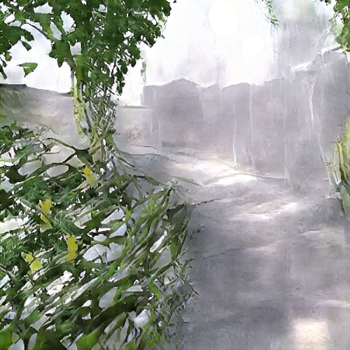
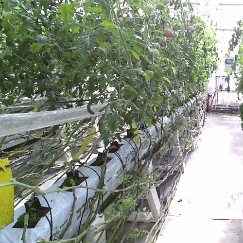
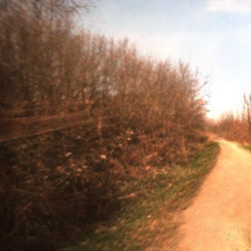
Fig. 1 shows real and synthetic urban scenes as well as a greenhouse scene for comparing the difference of appearance. The difference between real and synthetic urban scenes (Figs. 1 and 1) mainly stems from the discrepancy of their characteristics of appearance such as textures. However, they share a similar distribution of the objects in the images, e.g., the majority of areas are occupied by buildings and roads. On the other hand, the images of real urban scenes and the greenhouses (Figs. 1 and 1) are both real, but there are instead structural differences such as the distribution and scales of the objects in the images, etc. These structural differences of the datasets makes the existing UDA methods less effective. In fact, as later shown in Sec. 4.3, state-of-the-art UDA methods result in poor performance.
While the outputs of the source models contain a lot of noise, we also observed that all the models provide accurate classification on large areas of the images (more details are in Sec. 3.3). Based on the observation, we propose to exploit multiple datasets as source datasets for pseudo-label generation, rather than relying on a single dataset dissimilar to the target dataset. Our key contribution is the method to generate pseudo-labels using models trained with multiple publicly available datasets to effectively transfer knowledge to structurally different target images without ground truth labels. Pseudo-labels for the target images are generated by merging outputs from multiple models, each of which is pre-trained with a labeled source dataset. In particular, a pseudo-label is assigned on a pixel only when all the source models predict the pixel as the same object class. This method effectively filters out misclassified labels and leads to a better performance of the trained models. To further suppress the effect of noise in the pseudo-labels, we also introduce a loss weighting based on the uncertainty of estimation and pseudo-label denoising inspired by Zheng et al. [7] and Zhang et al. [8], respectively.
We demonstrate the effectiveness of the method in the experiments of adaptation from three source datasets of urban or outdoor scenes, to multiple greenhouse datasets as the target.
2 Related work
2.1 Semantic segmentation
2.1.1 DNN architecture
Semantic segmentation is a task to predict an object class on each pixel of an image. It is one of the most important tasks in the field of computer vision and its application includes scene recognition for the navigation of self-driving cars and autonomous mobile robots. After Long et al. [9] proposed the idea of converting classification networks into a fully convolutional network to produce a probability map for the input of arbitrary size, most of the semantic segmentation models have been developed based on it [10, 11]. Many recent high accuracy models use ResNet proposed by He et al. [12] as a backbone network to build very deep networks [13, 14]. While it is proven to be effective to stack many layers to get a high accuracy, the performance comes at the high computational cost. To tackle this problem, computationally efficient models have also been studied, targeting the applications such as robotics and autonomous driving cars where real time recognition is required for the operation [15, 16, 17, 18].
2.1.2 Semantic segmentation for navigation in agriculture
Image segmentation techniques have been studied for navigation tasks in agricultural fields. Lulio et al. [19] proposed an image segmentation method for robot navigation in orchards with a combination of color-based region segmentation and an artificial neural network. Sharifi et al. [20], Aghi et al. [21], and Lin et al. [22] proposed DNN-based segmentation methods for the purpose of robot navigation.
In contrast to “shallow” methods, the DNN-based methods have several advantages. First, the generalization performance of DNNs is better than that of the image processing methods and machine learning methods with hand-crafted features. Second, the trained DNNs provide discriminative “deep” features that can be used in other tasks [23]. In fact, we used the features learned in the proposed method to estimate the traversability of the objects and showed that the features are capable of discriminating between traversable and non-traversable plants [2].
Moreover, unlike other DNN-based methods, our proposed methods do not require any image datasets with manually provided labels dedicated for the target environment, i.e., greenhouses.
2.2 Domain adaptation for semantic segmentation
2.2.1 Unsupervised domain adaptation
Semantic segmentation based on deep learning usually requires a large amount of training data labeled on each pixel and manual labeling is especially time-consuming. One promising approach is to use a large amount of image-label pairs automatically synthesized by computer graphics. Since the appearance of the synthetic images is different from real-world images, the model trained on the synthetic data does not perform well in the real world. Therefore, we need UDA to re-train the model in a different domain i.e., the real environment. There are two major approaches to UDA methods [24, 25]. One is called “domain alignment” where a model is trained so that the distribution discrepancy of domains is minimized. The alignment is done in different levels such as the input space [26, 27], feature space [28, 29], and output label space [30, 31]. Those methods aim to learn domain-invariant features of both domains. Recently, such training is often realized by adversarial training [32, 29].
The other approach of UDA is pseudo-label-based methods. This type of method uses outputs from a model pre-trained with a source dataset as true labels. By directly training the model on the target images with the pseudo-labels, it can fully learn domain-specific information. However, the pseudo-labels for the target images inevitably contain misclassification and it may affect the training as noise. To deal with the noise, different approaches have been proposed, such as thresholding based on the confidence of the prediction [33, 34], the adaptive weighting of loss values based on the uncertainty of the prediction [7], and prototype-based pseudo-label denoising [8].
2.2.2 Multi-source domain adaptation
Apart from the aforementioned single-source adaptation methods, there are several studies of multi-source domain adaptation (MDA). Mansour et al. stated that the target distribution can be represented as a weighted mixture of multiple source distributions. Following this analysis, Xu et al. [35] implemented an MDA training with deep networks. For a detailed survey of MDA, readers are referred to Zhao et al. [36]. Zhao et al. [37] extended Cycada [26] to MDA for semantic segmentation. A work of Nigam et al. [38] utilizes multiple models trained with different source datasets as feature extractors, and adapt the segmentation layers to a target dataset of overhead images from a drone. Although their method is similar to ours in a way that multiple pre-trained networks are exploited, their task is supervised domain adaptation where they prepare their own labeled dataset, while our method utilizes publicly available datasets that are not specifically built for greenhouse scenes.
2.2.3 Benchmarks
As a benchmark of semantic segmentation, a task considered de-facto standard is adaptation from synthetic datasets such as the GTA5 dataset [4] and the SYNTHIA dataset [5] to a real dataset, most often Cityscapes dataset [6]. In this task, scenes are limited to urban scenes in both the source datasets and the target datasets. Besides, the set of object classes is identical in all the datasets. In this paper, we further investigate the methodology of transferring knowledge in cases where the structure of the environments is different, and the source and the target datasets do not share their label space.
3 Proposed method
3.1 Overview
The purpose of this work is to train a semantic segmentation model that achieves low error on greenhouses images without hand-annotated labels. To this end, we consider using multiple publicly available labeled image datasets as source datasets to transfer knowledge to the target images. Specifically, we use datasets of urban scenes and outdoor scenes, namely, CamVid dataset [39], Cityscapes dataset [6], and Freiburg Forest dataset [40], as source datasets. Each source dataset has a different set of object classes. The target datasets are greenhouse images with the following classes: plant, artificial object, and ground. The target datasets do not have any label data for supervision.
Formally, we assume source datasets and an unlabeled dataset . A source dataset consists of an image set and a set of corresponding segmentation label maps , where denotes the number of images in . The source datasets can have a different number of object classes. The target dataset consists of only an image set , where denotes the number of images in .
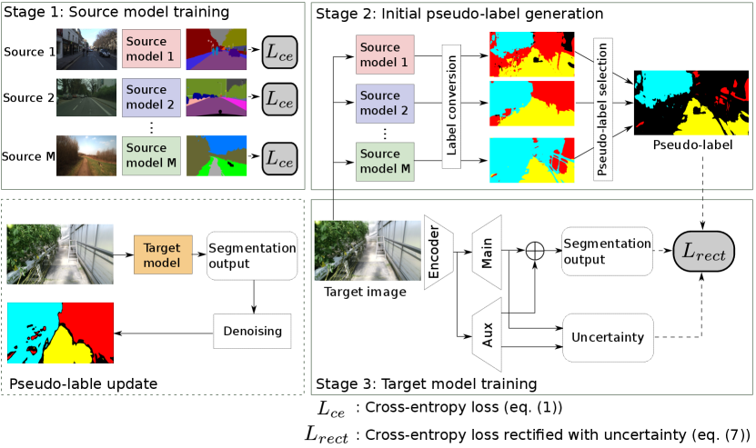
Fig. 2 shows the overview of the proposed method. It consists of three stages. The first stage is the training of source models. For each source dataset, a segmentation model is trained in a supervised manner. In the second stage, the target images are fed into the source models and pseudo-labels are generated by merging the outputs from the source models. An output from each source model is first converted to the target labels using a label conversion function, which is heuristically defined. The pseudo-labels are then generated by selecting the labels that the models unanimously predict as the same label. Finally in the third stage, the target model is trained with the pairs of the target images and corresponding pseudo-labels. The classification loss is adaptively weighted by the uncertainty of the prediction as proposed in [7]. During the training, the pseudo-labels are updated using the outputs from the currently trained model for further leveraging the knowledge learned from the initial pseudo-labels. In the pseudo-label update, a denoising method inspired by [8] is used.
In our method, we employ ESPNetv2 [16], a light-weight semantic segmentation model, as base network architecture for its suitability to real-time scene recognition of mobile robots. The proposed method, however, is not dependent on a specific network architecture.
3.2 Model pre-training
We first train a segmentation model on each source in a fully supervised manner. In this step, each model is trained with the original classes in the corresponding source dataset. A standard cross entropy loss is used as a loss function:
| (1) |
where denotes the probability of class at the location for an image predicted by the segmentation model with weights , and denotes a one-hot label at pixel . A source model for dataset is initialized as follows:
| (2) |
Usually, in loss calculation, greater weight is set for the loss of rarer classes in order to deal with class imbalance. For our task, however, we empirically found that a model provides more accurate pseudo-labels when the model is trained with a weight proportional to the frequency of the label, which is contrary to the usual practice. We suppose the reason is as follows. The usual loss weighting is mainly for capturing relatively small objects such as road signs and poles. In our target environment, i.e., greenhouses, such a fine-grained perception is not necessary because the space of the environment is fixed and thus the variation of the scale of the objects is limited. Moreover, the object classes in the target datasets are coarse. Therefore, the usual practice of training may lead to a model that is overly focused on small objects which is unnecessary for the pseudo-label generation.
3.3 Pseudo-label generation using multiple pre-trained models
3.3.1 Underlying idea
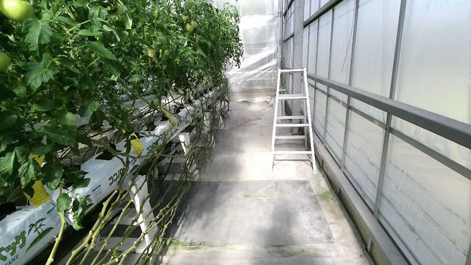
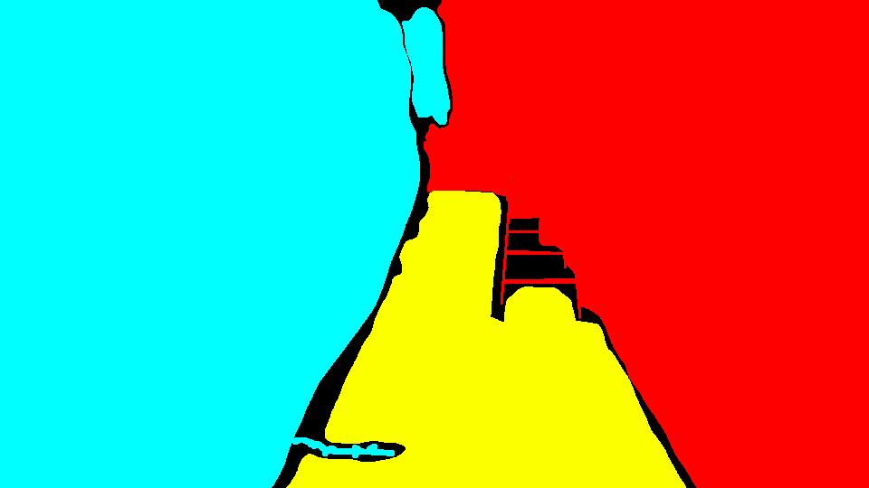
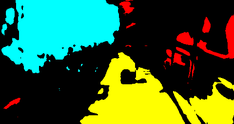
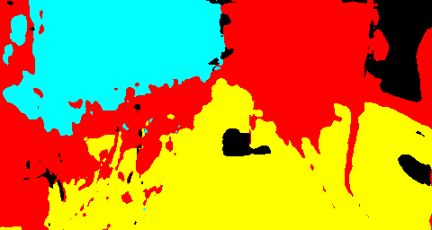
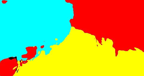
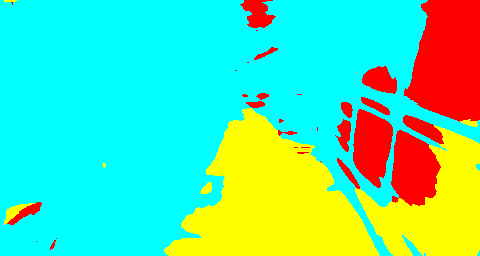
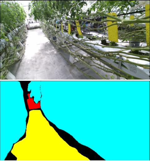
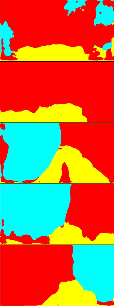
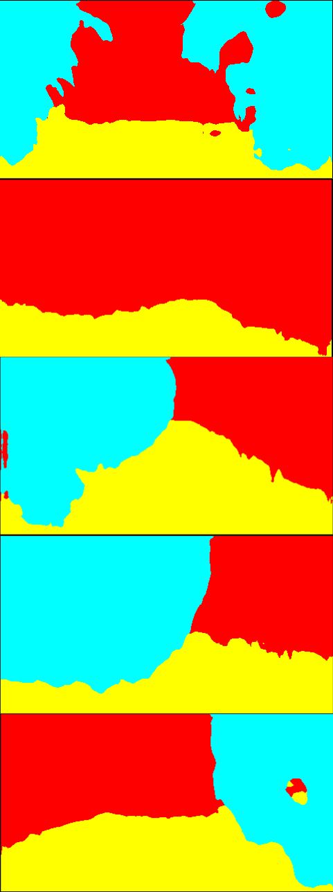
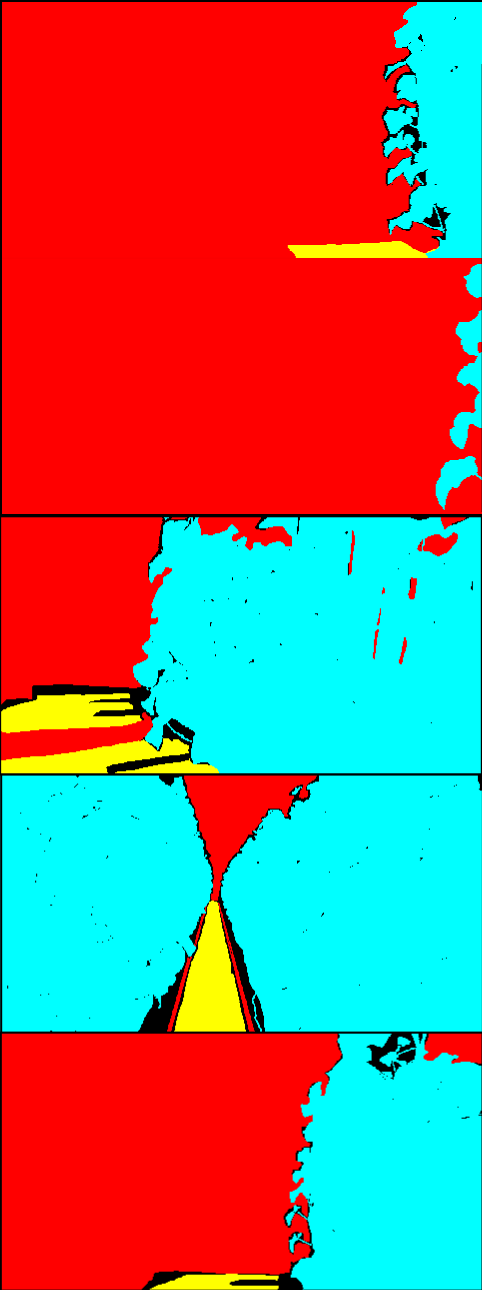
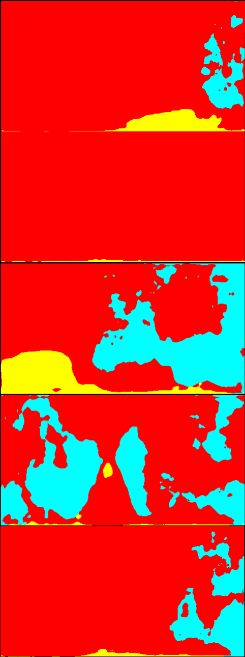
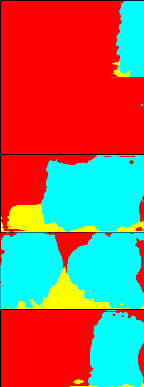
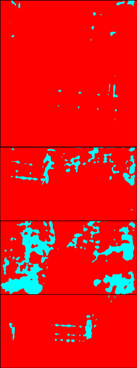
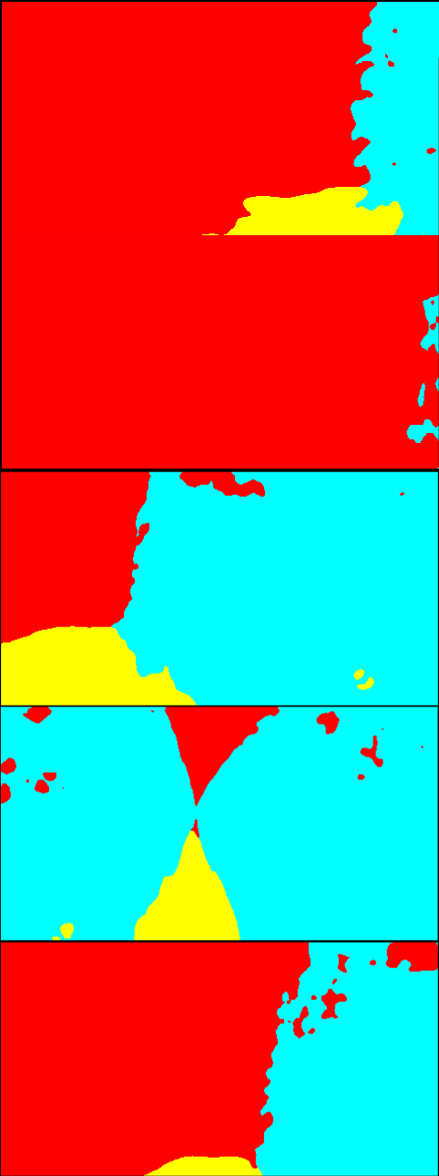
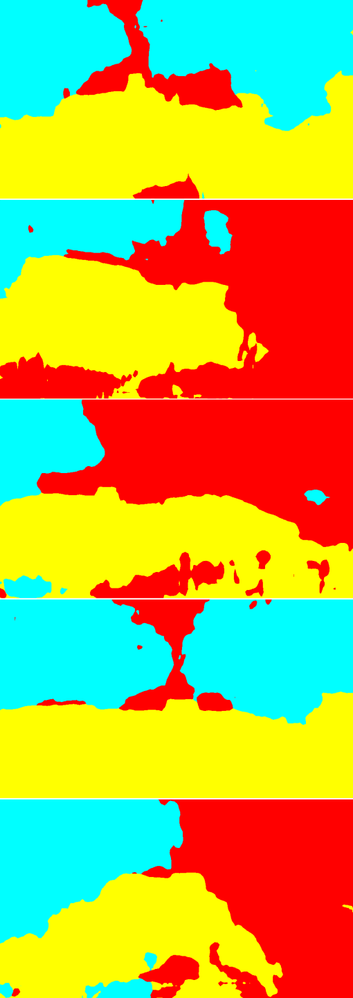
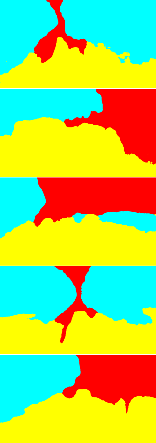
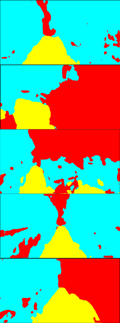
Our intuition behind this method of multi-source pseudo-label generation is that while the prediction from each source model contains a lot of misclassifications, the models correctly predict many of the pixels in common. Fig. 3 shows outputs for a target image from different source models trained with the CamVid dataset [39], Cityscapes dataset [6] and the Freiburg Forest dataset [40] as well as the target image, hand-labeled ground truth, and the pseudo-label generated from the three outputs. As can be seen in Fig. 3, many of the true regions of “plant” class and “ground” class are correctly classified in all the models. This implies that getting a consensus of the models is effective for generating precise pseudo-labels as shown in Fig. 3. Another thing worth noting is that each model has its own characteristics of prediction. For example, the prediction of the model trained with Freiburg Forest dataset on the ground regions better captures the shape of true ground regions than the other two models. However, the prediction on the plants and artificial objects is not accurate. On the other hand, in the model trained with Cityscapes, the prediction on the ground region includes a lot of false positives, while that on the other objects is more accurate than the Freiburg Forest model. These differences stem from the structural differences of the source datasets. The proposed method avoids biased training to the structural features of a specific source dataset dissimilar to the target by getting agreements of multiple source models.

3.3.2 Pseudo-label generation method
In this step, pseudo-labels for the target images are generated using outputs from the models pre-trained with the source datasets. First, the target images are fed in all the pre-trained models to yield predicted labels in the label space of each source domain. The predicted label from the model of source for the th target image is given as follows:
| (3) |
The predicted labels are then mapped to the target label space using a label conversion function , where and denote a set of labels in source and target , respectively:
| (4) |
Here, we heuristically define the mapping from the source classes to the target classes for each source domain as shown in Table 1. After the label conversion, for each pixel of the target images, a predicted label is assigned to the pixel if the prediction is the same among all the source models. Otherwise, “other” label is assigned and not used for training. Formally, a pseudo-label for the pixel of the th target image is generated as follows:
| (5) |
where is a class category in the target dataset and is a class label “other” that is not used for loss calculation during the training and thus does not affect the training.
3.4 Model training on the target data
We train a segmentation model with the target images and the corresponding pseudo-labels. Although the valid labels in the pseudo-labels generated in Sec. 3.3 are unanimously predicted by the source models and thus highly likely correct, we introduce uncertainty-based loss weighting and prototype-based pseudo-label denoising for further suppressing the effect of noise in the pseudo-labels.
3.4.1 Loss weighting based on the uncertainty of estimation
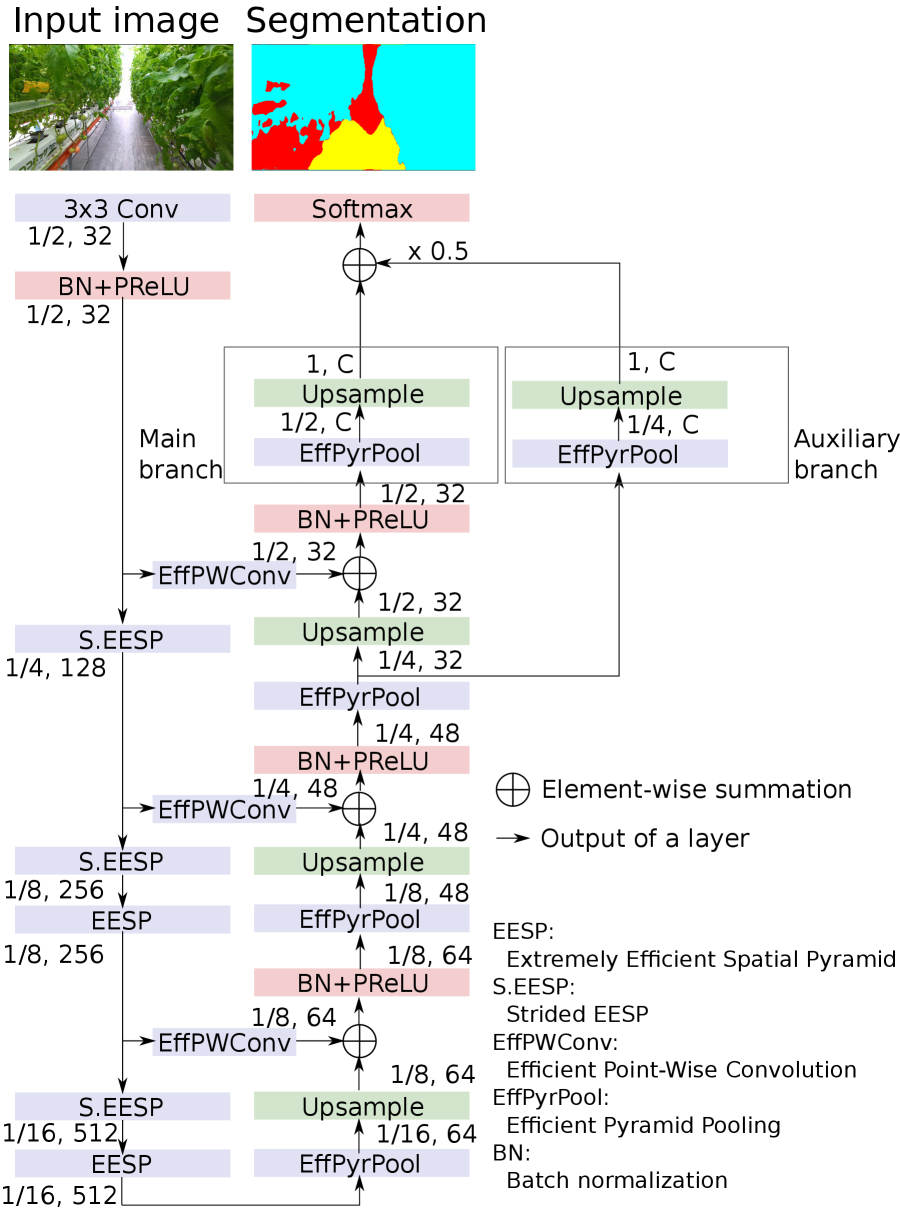
In standard training of semantic segmentation models, the cross entropy loss is widely used. In the training with pseudo-labels, however, equally treating all the pseudo-labels may lead to poor performance due to noise in the pseudo-labels. Zheng et al. [7] proposed an adaptive loss weighting that decays as the uncertainty of the estimation increases so that the losses on the pixels with high uncertainty do not affect the training much. Their method exploits an auxiliary segmentation branch to predict pixel-wise uncertainty of the label prediction. We attach an auxiliary segmentation branch to ESPNetv2 for uncertainty estimation. The entire segmentation network is shown in Fig. 7 in Appendix 6.
Given the output of primary branch and that of the auxiliary branch , the uncertainty of the prediction is defined as Kullback-Leibler Divergence (KLD) of the distributions of class probabilities from the two branches:
| (6) |
Using eq. (6), the loss function is defined as follows:
| (7) |
3.4.2 Prototype-based pseudo-label denoising
In the middle of the training, we update the pseudo-labels with the outputs from the current model to further leverage the knowledge learned from the initial pseudo-labels. We introduce pseudo-label updating with prototype-based denoising inspired by Zhang et al. [8].
At first, the prototypes are calculated. The prototype of class is a mean of the features that belong to the class and is calculated using the current pseudo-labels as follows:
| (8) |
where is an intermediate feature provided by the currently trained model at pixel , and is the indicator function that returns 1 when its argument is true and 0 otherwise.
Pseudo-labels for image are then updated as follows:
| (9) |
where is a normalization factor and is a threshold for pseudo-label selection, which is set to 0.9 in the experiments. is a vector of weight values to modulate the class probabilities, calculated using the distances between the feature and each prototype. For each pixel, the weight is calculated as follows:
| (10) |
where is a temperature parameter that controls the degree of bias of the distribution, which is set to 1 in [8]. The values of indicate the class likelihood of the feature based on the distance from the feature to each prototype, and the probabilities predicted by are rectified by .
3.5 The overall algorithm
The overall algorithm is shown in Algorithm 1. As already mentioned, our training pipeline consists of three stages. A segmentation model for each source dataset is trained in standard supervised learning in the first stage and initial pseudo-labels for the target images are generated using the pre-trained models in the second stage. In the third stage, the target model is trained using the target images and the pseudo-labels. The training is done in several “rounds”, each of which consists of several epochs. Here, the number of epochs per round is set to 5, and the maximum number of rounds is set to 10.
During training, the pseudo-labels are updated using the target model currently being trained. In this work, we update the pseudo-labels once after the third round of training with the initial pseudo-labels because the training with the initial pseudo-labels converges by the third round. We compare the different pseudo-label update strategies in Sec. 4.5.
4 Experiments
| CamVid | Cityscapes | Forest | Greenhouse A, B, C | ||||||||||
|---|---|---|---|---|---|---|---|---|---|---|---|---|---|
| Tree | Vegetation |
|
Plant | ||||||||||
|
|
Obstacle | Artificial object | ||||||||||
|
|
Road | Ground | ||||||||||
|
|
Sky | Other (Not used in the training) |
4.1 Experimental setup
4.1.1 Training conditions
We use PyTorch implementation of ESPNetv2 [16]. For estimating uncertainty, an auxiliary segmentation branch is attached. The architecture is shown in Fig. 7 in Appendix 6. The processing time was about 44 [msec/image], or 23 [fps]. The number of floating point operations (FLOPs) is 0.79 [GFLOPs] while that of the original ESPNetv2 for semantic segmentation is 0.76 [GFLOPs] [16], indicating that attatching the auxiliary branch did not affect the computational efficiency. All training of the proposed method is performed on one NVIDIA Quadro RTX 8000 with 48GB RAM. The numbers of training rounds and epochs per round are set to 10 and 5, respectively. The learning rate is fixed to and the batch size is 48. Adam [41] is used as an optimizer. Weights of the target models are initialized by the supervised training of semantic segmentation on the CamVid dataset [39], except for the last classification layer initialized with random values. We measure segmentation performance with the Intersection over Union (IoU) metric.
4.1.2 Datasets
We use CamVid [39], Cityscapes [6] and Freiburg Forest dataset [40] (hereafter referred to as CV, CS, and FR, respectively) for the training of the source models. CV, CS, and FR have 367, 2975, and 230 labeled training images, respectively. Label conversions from the source datasets to the target datasets () are heuristically defined as shown in Table 1 . A more detailed analysis of the label mapping is in Appendix 7.
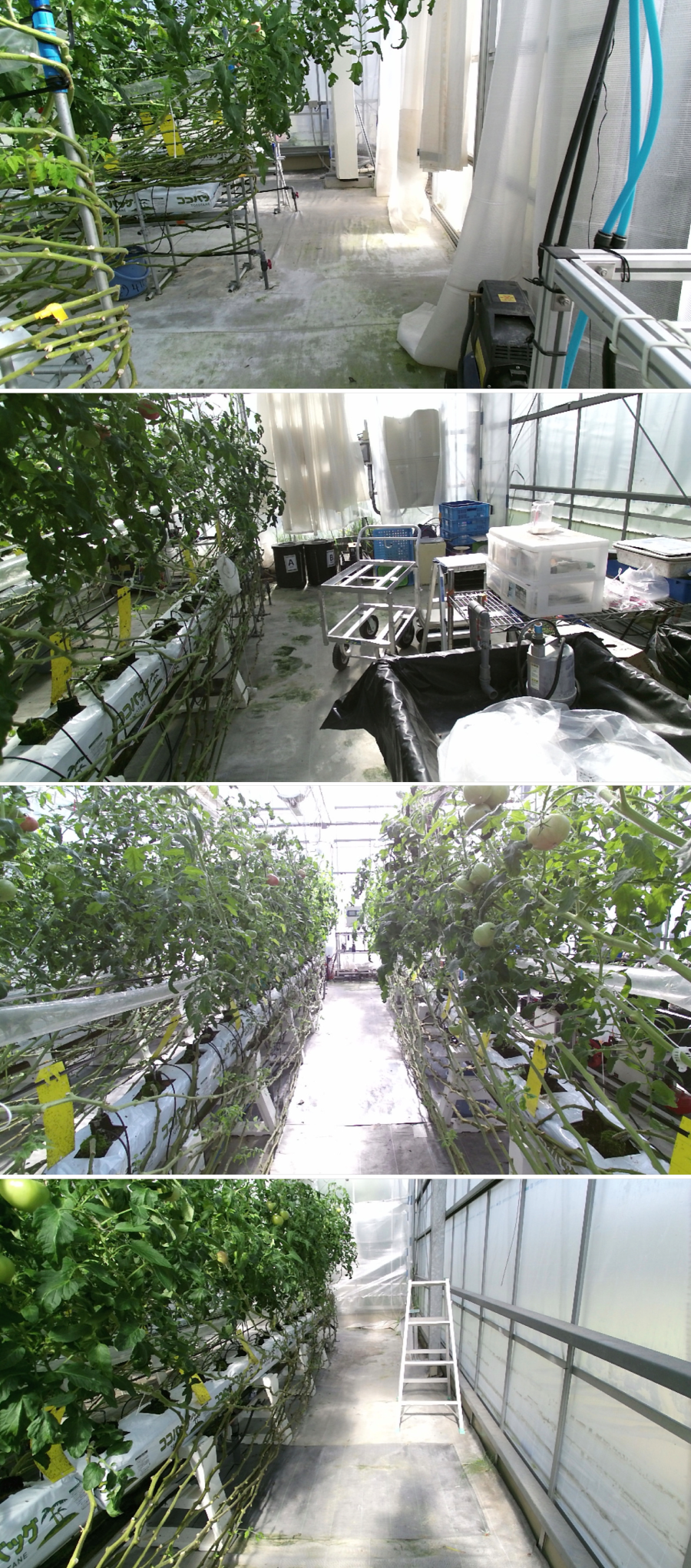
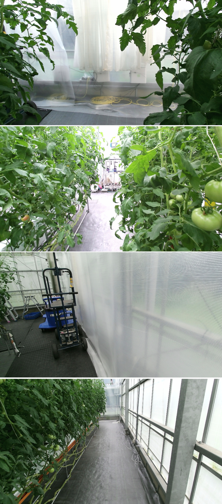
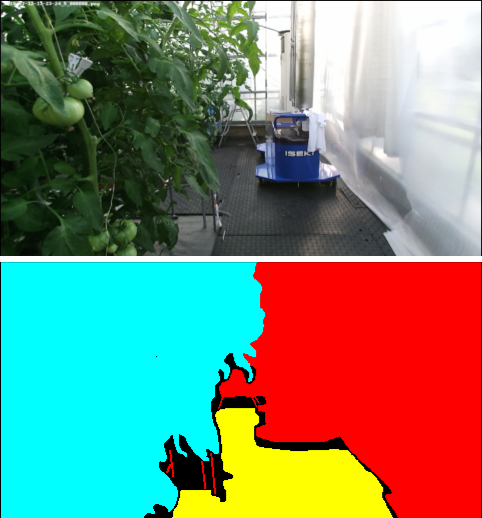
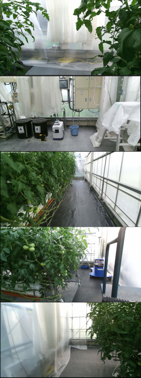
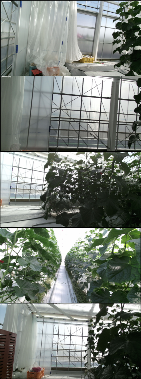
As target greenhouse datasets for adaptation, we acquired images from three greenhouses; Greenhouse A that grows tomatoes, Greenhouse B that is the same greenhouse as Greenhouse A but acquired in different date and time, and Greenhouse C that grows cucumbers. Each target dataset has 6689 unlabeled images. Example images of the target datasets are shown in Fig. 4.

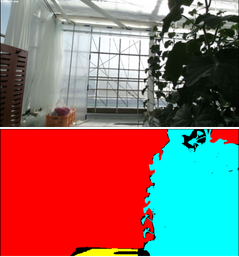
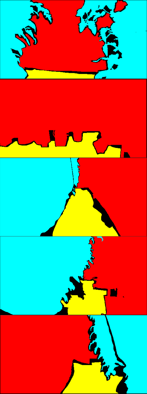
For each target dataset, we prepared test images with manually annotated labels for evaluation. The numbers of the test images are 100 for Greenhouse A, and 50 for B and C. The labels on the test images include the “other” class and the pixels with the class are not considered in the calculation of the metric (See Fig. 5). More detailed annotation policy is described in Appendix 8.
4.2 Comparison to single-source baselines
| Target | Source | Class IoU | mIoU | ||
| Plant | Artificial object | Ground | |||
| Greenhouse A | CV (no adapt) | 64.72 | 56.19 | 46.34 | 55.75 |
| CS (no adapt) | 63.71 | 68.71 | 36.37 | 56.26 | |
| FR (no adapt) | 60.24 | 45.27 | 30.49 | 45.33 | |
| CV | 70.21 | 68.66 | 57.10 | 65.32 | |
| CS | 60.17 | 71.47 | 31.02 | 54.22 | |
| FR | 52.73 | 50.68 | 40.84 | 48.11 | |
| CV+CS | 73.81 | 73.49 | 47.55 | 64.94 | |
| CS+FR | 79.50 | 76.35 | 70.32 | 75.39 | |
| FR+CV | 77.40 | 73.00 | 63.20 | 71.20 | |
| CV+CS+FR | 80.71 | 78.21 | 72.68 | 77.20 | |
| Greenhouse B | CV (no adapt) | 65.57 | 65.30 | 57.65 | 62.84 |
| CS (no adapt) | 83.33 | 80.09 | 49.68 | 71.03 | |
| FR (no adapt) | 48.47 | 54.34 | 19.17 | 40.66 | |
| CV | 71.37 | 77.15 | 62.73 | 70.42 | |
| CS | 83.49 | 77.39 | 44.53 | 68.47 | |
| FR | 47.04 | 58.60 | 42.87 | 49.50 | |
| CV+CS | 87.19 | 87.00 | 60.96 | 78.38 | |
| CS+FR | 82.56 | 89.44 | 70.60 | 80.87 | |
| FR+CV | 75.99 | 85.70 | 60.48 | 74.06 | |
| CV+CS+FR | 83.56 | 89.08 | 73.37 | 82.33 | |
| Greenhouse C | CV (no adapt) | 58.89 | 58.29 | 19.82 | 45.66 |
| CS (no adapt) | 79.09 | 81.10 | 18.11 | 59.43 | |
| FR (no adapt) | 61.65 | 49.24 | 25.56 | 45.48 | |
| CV | 69.96 | 70.30 | 22.52 | 54.26 | |
| CS | 85.51 | 85.30 | 21.86 | 64.23 | |
| FR | 66.00 | 65.52 | 0.6549 | 44.06 | |
| CV+CS | 88.76 | 87.20 | 28.61 | 68.19 | |
| CS+FR | 84.99 | 82.26 | 29.56 | 65.61 | |
| FR+CV | 91.12 | 90.00 | 45.12 | 75.41 | |
| CV+CS+FR | 91.16 | 88.84 | 40.67 | 73.56 | |
We conducted an experiment of adaptation from the source outdoor datasets to each of the target greenhouse datasets. In the single source baselines (CV, CS, and FR), the initial pseudo-labels were generated via the pseudo-label update procedure described in Sec. 3.4.2 in the source label space , followed by the label conversion by to map the labels to the target label space. All the models were trained with the initial pseudo-labels for the first three rounds. After that, the pseudo-labels were updated using the hard pseudo-labels with the prototype-based denoising and used in the rest of the training.
Table 2 shows the result of the training. The results of “no adapt” were provided by directly feeding the target images to the source models followed by the label conversion. Before the adaptation, the IoUs of the source models were low and not applicable to real applications. The performance of single-source training depended on the source dataset. In some cases, the adaptation resulted in improvement from the model without adaptation, while in some others the performance deteriorated after the adaptation. The cause of the degradation is that the training progressed in the wrong direction due to the noisy pseudo-labels. This indicates that the training with a single source may not be reliable enough when the source and target datasets have a large domain shift.
With our multi-source adaptation, on the other hand, the accuracy was significantly improved even though each source model is not reliable on the target data. The results show the ability of our method to transfer useful common knowledge about the appearance of objects from the source datasets to the target. The two-source training resulted in comparative or even better performance than the three-source training (CV+CS+FR). It is worth noting that the combination of different types of environments results in especially high accuracy, i.e., FR+CV and CS+FR. CV (CamVid) and CS (Cityscapes) are datasets of urban scenes, while FR (Freiburg Forest) consists of images of outdoor scenes with rough terrains and vegetation, This implies that we should use datasets with a high variety of environments as sources.
The most suitable combination, however, depends on the target dataset in the two-source setting. For example, CS+FR resulted in the second-best performance on Greenhouse A and B, while it was the worst among the multi-source settings on Greenhouse C. On the other hand, the three-source training consistently performed the best or the second-best on all the target datasets. We, therefore, suggest exploiting the three source datasets for the segmentation task in greenhouse environments.

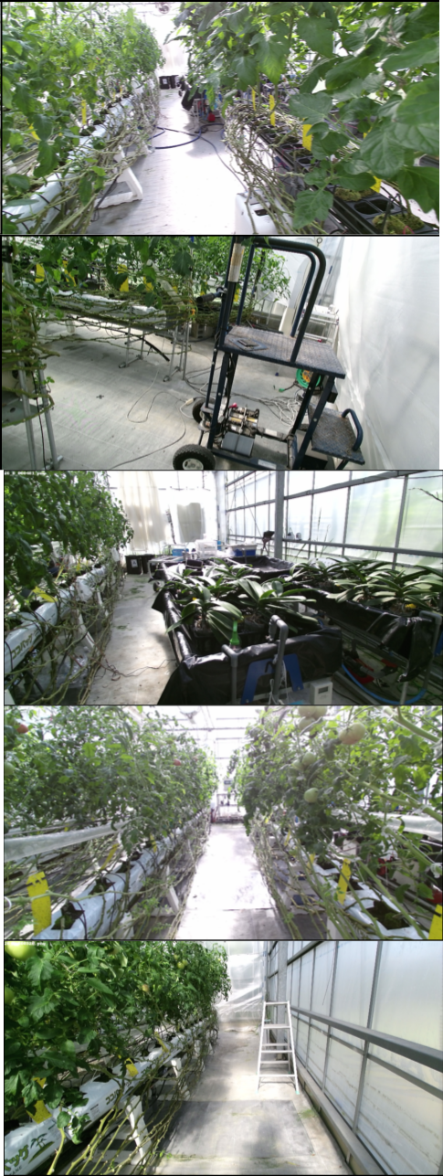

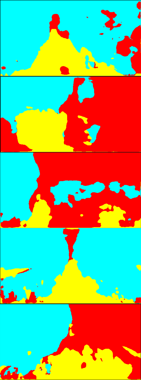
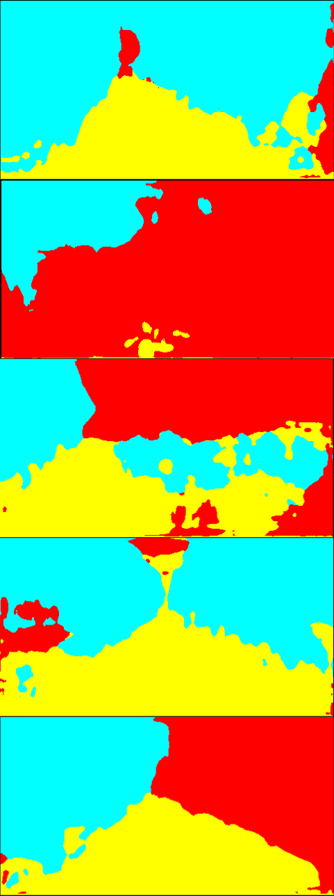
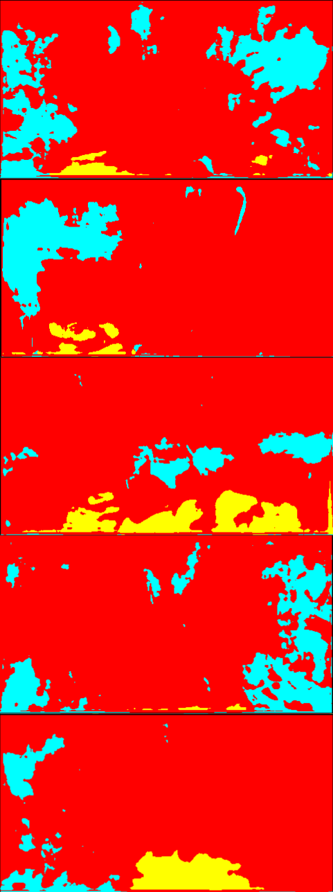

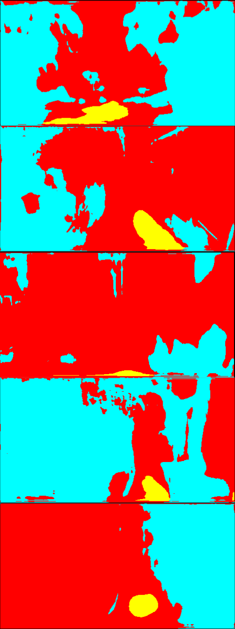
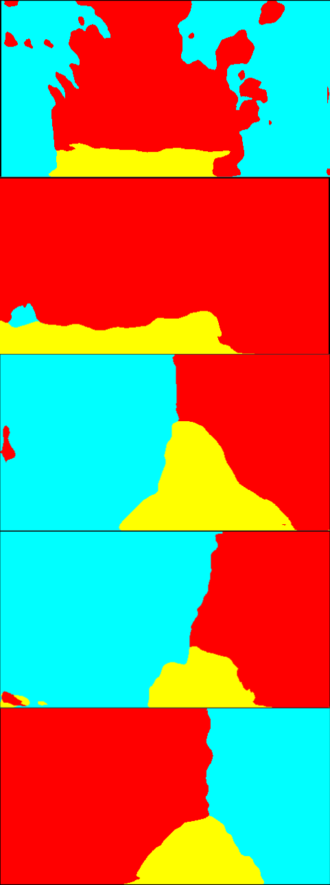
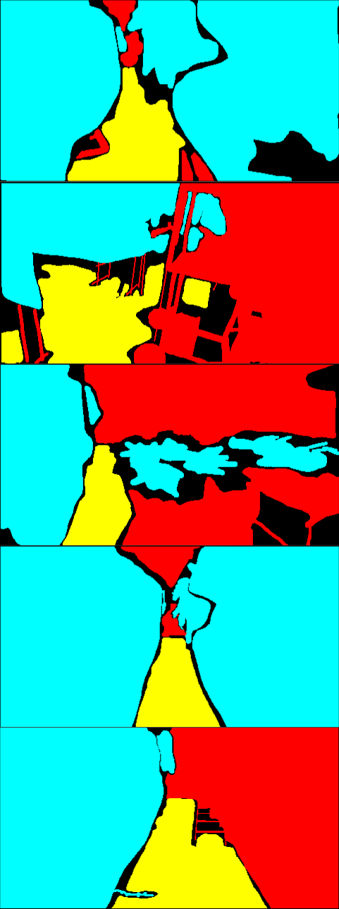
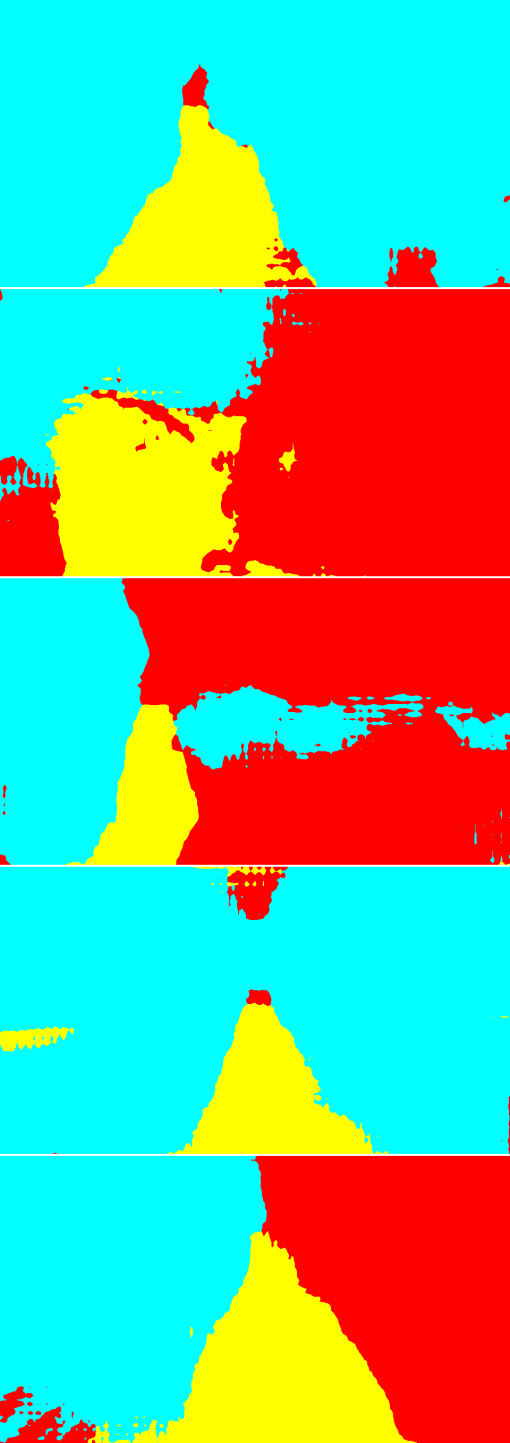
Fig. 6 is the result of the adaptation on Greenhouse A. In Fig. 6, while the results of the single-source training are relatively noisy, the multi-source ones provide smoother outputs. In particular, the plant regions are classified more accurately. Qualitatively, we suppose that this level of accuracy is sufficient for the operation of mobile robots. For Greenhouse B and C, the results are shown in Fig. 8 and 9 in Appendix 9. From Figs. 8 and 9, we can see that accurate segmentation can be achieved in other environments, and thus the knowledge that the proposed method transfers from the source datasets is applicable in a variety of greenhouse environments.
4.3 Comparison to existing methods
4.3.1 Baseline methods
To evaluate the relative performance of our proposed method, we conducted training with existing methods of supervised learning as well as single-source and multi-source UDA for semantic segmentation. Implementation details of the baseline methods are described in Appendix 10.
Supervised learning methods We introduce a supervised support vector machine (SVM) on superpixel features and a supervised DNN as supervised baselines. The SVM method is equivalent to some existing segmentation methods such as Sharifi et al. [20] and Lulio et al. [19], where an image is partitioned into small segments and then classified based on their hand-crafted features. As a DNN model, we use the architecture that is the same as the proposed method. We refer to the SVM method as SP-SVM and the DNN method as SP-DNN. Implementation details of SP-SVM are in Sec. 10.1.
For evaluation of the supervised baselines, we conducted 10-fold cross-validation with the 100 labeled images of Greenhouse A, which are used as the test data in the experiments of the UDA methods. The reported results are averages of IoUs on the test fold of each of the 10 training trials. Note that the training setting and the evaluation condition are different from the UDA training. This is due to the limited amount of manually labeled greenhouse images available. Nevertheless, we report the results of the supervised baselines to demonstrate baseline performances that we can expect from supervised learning.
UDA As existing UDA methods for semantic segmentation, we introduce representative UDA methods in different generations, i.e., confidence regularized self-training (CRST) [34] proposed in 2019, Seg-Uncertainty [7] and ProDA [8] proposed in 2021. They employ self-supervised learning with pseudo-labels, which is a popular approach in current UDA methods for semantic segmentation. Seg-Uncertainty and ProDA also involve GAN-based training based on [30] to further enhance the adaptation. Seg-Uncertainty and ProDA are the original works of the uncertainty-based loss weighting and the pseudo-label denoising in our method, respectively.
We used the source code distributed by the authors with modifications to apply them to our experiments, such as adding the new datasets and converting the source labels to the target label set defined in Table 1. In terms of ProDA, we report the result of stage 1 proposed in [8]. Although the original method employs knowledge distillation after stage 1 to boost the performance, they reported the state-of-the-art performance at the time with only the training of stage 1. We, therefore, suppose the result of stage 1 on our setting is sufficient as a baseline. The rest of the training process follows the algorithm of each method. Implementation details are in Appendix 10.2.
Although there are also multi-source UDA methods such as Multi-source Domain Adaptation for Semantic Segmentation (MADAN) [37], we could not train it due to limitations of computational resources. In Appendix 11.2, we show results of image style transfer between the source dataset and the target greenhouse dataset, which is the first step of MADAN.
4.3.2 Source datasets
In the comparative studies of single-source UDA methods, we report the results on Cityscapes (CS) since it provided best results than CV and FR) in all of the single-source baseline methods. We suppose this may be because CS has a sufficient amount of images (about 3000) for training models with a large capacity such as DeepLab v2, while the other source datasets (CV and FR) have only a few hundreds. On CV and FR, the model may have overfit to the training sets due to the scarcity of the data, and thus resulted in poorer adaptation performances. As there was no significant difference of adaptation performance between the source datasets in the single-source setting shown in Sec. 4.2 (see Table 2), we believe it is reasonable to use CS to demonstrate the performance of the baselines on behalf of the three source datasets.
4.3.3 Results
Table 3 shows the results.
| Method | Class IoU | mIoU | ||
| Plant | Artificial object | Ground | ||
| SP-SVM* | 74.99 | 54.66 | 53.54 | 61.06 |
| SP-DNN* | 86.27 | 78.64 | 88.49 | 81.68 |
| CRST [34] | 78.89 | 76.85 | 65.10 | 73.62 |
| Seg-Uncertainty [7] | 52.17 | 70.68 | 27.29 | 50.04 |
| ProDA [8] | 56.15 | 60.81 | 28.53 | 48.50 |
| CV+CS+FR (Proposed) | 80.71 | 78.21 | 72.68 | 77.20 |
Overall, the proposed method outperformed the baseline methods except for SP-DNN, and thus exhibited the ability to transfer knowledge from the datasets dissimilar to the target dataset. Although the performance of the baseline methods might be improved with extensive hyper-parameter search, the results indicate that relying on a single source is not effective enough even when using state-of-the-art UDA methods in our task where the source and target datasets do not share their structure of the scenes. Qualitative results are shown in Appendix 11. While SP-DNN resulted in the best IoUs, it also showed a clear tendency of overfitting due to the scarcity of training data. Although increasing the training data will resolve the problem, it requires laborious manual annotation. On the other hand, the proposed method enables training with a large amount of unlabeled images and provides a comparative performance.
Among the baseline UDA methods, CRST resulted in better performance than others, although they are reported to be better than CRST [7, 8]. We conjecture that adversarial learning negatively contributed to these results. ProDA and Seg-Uncertainty involve adversarial learning in the training processes to make the spatial structure in the output space as close as possible between the source and the target datasets [30]. Adversarial learning, including GANs [32], is effective when the difference between the source and the target stems mainly from the styles such as texture and color and the datasets share similar structure. For instance, GANs can be used to transfer the image style of source images closer to the target images without significantly changing the image contents, i.e., semantic class of corresponding image regions, so that a segmenter for the target images can be trained on the transferred source images in the target’s style with the ground truth labels. However, when the structure of the scenes is different, adversarial learning does not necessarily convey meaningful information. In fact, as shown in Appendix 11.2, the image contents are not preserved between the original and the translated images after CycleGAN-based image style transfer between CS/FR and Greenhouse A. For example, some ground regions in CS are transferred to green plant-like stuff, and some plant regions are transferred to regions with sky-like appearance (See Fig. 11). In [37], the authors also pointed out that the structural differences of objects between the source and the target datasets led the training to poor performances on those object classes (e.g., the source in target images are much taller than those in target images). Those facts imply adversarial learning is not as effective for adaptation under such structural differences between the source and the target scenes.
4.4 Comparison of strategies to merge multi-source information
| Majority | Unanimity (proposed) |
| 70.03 | 77.20 |
To see the validity of the proposed pseudo-label generation based on unanimity of the source models, we conducted training with a different strategy, namely majority-based pseudo-label generation. In the majority-based strategy, a label is assigned to a pixel when more than two source models of the three predict the pixel as the same object class.
The results are shown in Table 4. The training with the majority-based pseudo-labels resulted in a significant drop in performance compared to the unanimity-based method. We suppose that since the majority-based method more aggressively involves pixels in the pseudo-labels, more noise was included and it affected the training. We can conclude that the pseudo-labels should be chosen carefully through the strict unanimity criteria for better training. Although the pseudo-labels generated in such a way become coarse, the model trained with them provides reasonable predictions as shown in the aforementioned experiments. The validity of training with coarse labels is also reported in [42].
4.5 Effect of updating the pseudo-labels
We evaluate the effect of pseudo-label update strategies. We compare the strategies as follows.
-
•
Initial the initial pseudo-labels are used throughout the training.
-
•
Update once the pseudo-labels are updated after three rounds (i.e., 15 epochs).
-
•
Update every round the pseudo-labels are updated every round after the first three rounds.
The results are shown in Table 5.
| Initial | Update once | Update every round |
| 75.44 | 77.20 | 74.82 |
Update once outperformed the other strategies. We suppose the reason is as follows. The initial pseudo-labels are sparse and many pixels are ignored in training. Although it plays a crucial role to transfer primary knowledge from multiple source datasets, using such labels throughout the training leads to a suboptimal result. Updating the pseudo-labels with Update once strategy enables to exploit the knowledge learned through the training with the initial pseudo-labels and involve more pixels in the training to further improve the performance.
While the label update improved the performance, updating the labels every round resulted in the worst IoU. This is an expected result because the pseudo-labels inevitably include wrong ones due to misclassifications and the errors are accumulated as the pseudo-labels are updated by the model trained with them. This problem is also pointed out in [8]. We, therefore, conclude that the pseudo-labels should be updated once in the early stage of the training.
4.6 Ablation on pseudo-label noise suppression strategies
We conducted an ablation study on the methods for noise suppression. We examined the methods as follows: confidence thresholding, loss weighting, and prototype-based denoising. The confidence thresholding is simply removing outputs with a confidence value below a predefined threshold from the pseudo-labels. Here, the confidence threshold is set to 0.9 in all the settings. The loss weighting and the prototype-based denoising are the methods described in Sec. 3.4.1 and 3.4.2, respectively.
We report the training results on Greenhouse A. The results are shown in Table 6.
| Confidence threshold | Loss weighting [7] | Prototype-based denoising [8] | mIoU |
| 73.95 | |||
| ✓ | 74.66 | ||
| ✓ | ✓ | 75.89 | |
| ✓ | ✓ | 75.53 | |
| ✓ | ✓ | ✓ | 77.20 |
The strategies for suppressing the effect of noise in pseudo-labels effectively improved the training performance. The combination of the loss weighting and the prototype-based pseudo-label denoising on top of the simple confidence thresholding resulted in the best performance. We, therefore, adopted this setting to all the other training we report in this paper.
4.7 Parameter sensitivity analysis
| 0.7 | 0.8 | 0.9 | 0.95 | |
|---|---|---|---|---|
| mIoU | 76.87 | 77.16 | 77.20 | 76.63 |
We analyze the effect of the confidence threshold in the pseudo-label generation. We trained models with different thresholds on Greenhouse A dataset. The results are shown in Table 7. resulted in the best performance. However, the difference among the parameters is less than one point and thus the method did not show significant sensitivity to the parameter choice.
4.8 Discussions
Here, we list the limitations of the proposed method.
-
1.
The limitation of the pseudo-label generation strategy
In the proposed method, pseudo-labels are selected for training only when all the source models unanimously make predictions on the corresponding pixels. Although such a conservative strategy contributed to removing noise as shown in Sec. 4.4, it may also result in lack of valid labels if one of the source datasets do not agree with others. This fact also hinders increasing the number of source datasets since the more the source models are, the harder it becomes to get agreement of all the source models and thus the produced pseudo-labels become too sparse.
-
2.
The limitation of applicable environments
In this paper, we confirmed that the proposed method is applicable to multiple greenhouses with a similar structure. We are now looking to apply our method to unstructured outdoor scenes. We have not confirmed that the same method also works for such scenes. We should, therefore, investigate the applicability of the proposed method to other scenes, e.g., unstructured outdoor scenes and forests.
-
3.
The limitation of capability to learn novel object classes
There may be cases where the target dataset has classes that do not appear in the source datasets, e.g., objects specific to the environment. The proposed method is not capable of learning such novel objects.
5 CONCLUSIONS
In this paper, we tackled a task of unsupervised domain adaptation from multiple outdoor datasets to greenhouse datasets, to train a model for scene recognition of agricultural mobile robots. We considered using multiple publicly available datasets of outdoor images as source datasets since it is difficult to prepare synthetic datasets of greenhouses as done in conventional work. To effectively exploit the knowledge from the source datasets whose appearance and structure is very different from the target environment, we proposed a pseudo-label generation method that takes outputs from each source model and selects only the labels that are unanimously predicted by all the source models. By the combination of our pseudo-label generation method and conventional methods, training of semantic segmentation on the greenhouse datasets is enabled without manual labeling of images. This contributes to reducing the burden of applying a visual scene recognition system of mobile robots in greenhouses. In fact, we have already applied the model trained with the proposed method to the recognition of a mobile robot for autonomous navigation [2].
Disclosure statement
The authors report there are no competing interests to declare.
Funding
This work is supported by Knowledge Hub Aichi Priority Research Project (third term). The work of Shigemichi Matsuzaki is also supported in part by the Leading Graduate School Program, “Innovative program for training brain-science-information-architects by analysis of massive quantities of highly technical information about the brain,” by the Ministry of Education, Culture, Sports, Science and Technology, Japan.
Authors’ biography
Shigemichi Matsuzaki received the associate degree in engineering from National College of Technology, Kumamoto College in 2016, and the bachelor’s and the master’s degrees in engineering from Toyohashi University of Technology, Aichi, Japan in 2018 and 2020, respectively. He is currently pursuing the Ph.D. degree at Toyohashi University of Technology. His research interests include deep learning in robot perception, mobile robots in unstructured environments, and mobile service robots.
Jun Miura received the B.Eng. degree in mechanical engineering, and the M.Eng. and Dr.Eng. degrees in information engineering from The University of Tokyo, Tokyo, Japan, in 1984, 1986, and 1989, respectively. In 1989, he joined the Department of Computer-Controlled Mechanical Systems, Osaka University, Suita, Japan. Since April 2007, he has been a Professor with the Department of Computer Science and Engineering, Toyohashi University of Technology, Toyohashi, Japan. From March 1994 to February 1995, he was a Visiting Scientist with the Computer Science Department, Carnegie Mellon University, Pittsburgh, PA. He has published over 240 articles in international journal and conferences in the areas of intelligent robotics, mobile service robots, robot vision, and artificial intelligence. He received several awards, including the Best Paper Award from the Robotics Society of Japan, in 1997, the Best Paper Award Finalist at ICRA-1995, and the Best Service Robotics Paper Award Finalist at ICRA-2013
Hiroaki Masuzawa received the associate degree in engineering from National College of Technology, Hachinohe College in 2006, received the bachelor’s and the master’s degree in engineering from Toyohashi University, Aichi, Japan in 2008 and 2010, respectively. He is currently a project research associate of Department of Computer Science and Engineering, Toyohashi University of Technology. His research interests include application of artificial intelligence to agricultural robots.
References
- [1] Matsuzaki S, Masuzawa H, Miura J, Oishi S. 3D Semantic Mapping in Greenhouses for Agricultural Mobile Robots with Robust Object Recognition Using Robots’ Trajectory. In: Ieee international conference on systems, man, and cybernetics. 2018. p. 357–362.
- [2] Matsuzaki S, Masuzawa H, Miura J. Image-Based Scene Recognition for Robot Navigation Considering Traversable Plants and Its Manual Annotation-Free Training. IEEE Access. 2022;10:5115–5128.
- [3] Csurka G. Domain Adaptation in Computer Vision Applications. Advances in Computer Vision and Pattern Recognition. Cham: Springer International Publishing. 2017.
- [4] Richter SR, Vineet V, Roth S, Koltun V. Playing for Data: Ground Truth from Computer Games. In: European conference on computer vision. Vol. 9906. 2016. p. 102–118.
- [5] Ros G, Sellart L, Materzynska J, Vazquez D, Lopez AM. The SYNTHIA Dataset: A Large Collection of Synthetic Images for Semantic Segmentation of Urban Scenes. In: Ieee/cvf conference on computer vision and pattern recognition. 2016. p. 3234–3243.
- [6] Cordts M, Omran M, Ramos S, Rehfeld T, Enzweiler M, Benenson R, Franke U, Roth S, Schiele B. The Cityscapes Dataset for Semantic Urban Scene Understanding. In: Ieee/cvf conference on computer vision and pattern recognition. 2016. p. 3213–3223.
- [7] Zheng Z, Yang Y. Rectifying Pseudo Label Learning via Uncertainty Estimation for Domain Adaptive Semantic Segmentation. International Journal of Computer Vision. 2020;129:1106–1120.
- [8] Zhang P, Zhang B, Zhang T, Chen D, Wang Y, Wen F. Prototypical Pseudo Label Denoising and Target Structure Learning for Domain Adaptive Semantic Segmentation. In: Ieee/cvf conference on computer vision and pattern recognition. 2021. p. 12414–12424.
- [9] Long J, Shelhamer E, Darrell T. Fully Convolutional Networks for Semantic Segmentation. In: Ieee/cvf conference on computer vision and pattern recognition. 2015. p. 3431–3440.
- [10] Badrinarayanan V, Kendall A, Cipolla R. SegNet: A Deep Convolutional Encoder-Decoder Architecture for Image Segmentation. IEEE Transactions on Pattern Analysis and Machine Intelligence. 2017;39(12):2481–2495.
- [11] Ronneberger O, Fischer P, Brox T. U-Net: Convolutional Networks for Biomedical Image Segmentation. Medical Image Computing and Computer-Assisted Intervention. 2015;9351:234–241.
- [12] He K, Zhang X, Ren S, Sun J. Deep Residual Learning for Image Recognition. In: Ieee/cvf conference on computer vision and pattern recognition. 2016 may. p. 770–778.
- [13] Zhao H, Shi J, Qi X, Wang X, Jia J. Pyramid scene parsing network. In: Ieee/cvf conference on computer vision and pattern recognition. 2017. p. 6230–6239.
- [14] Chen Y, Li W, Chen X, Gool LV. Learning Semantic Segmentation from Synthetic Data: A Geometrically Guided Input-Output Adaptation Approach. In: Ieee/cvf conference on computer vision and pattern recognition. 2019. p. 1841–1850.
- [15] Mehta S, Rastegari M, Caspi A, Shapiro L, Hajishirzi H. ESPNet: Efficient Spatial Pyramid of Dilated Convolutions for Semantic Segmentation. In: European conference on computer vision. 2018. p. 561–580.
- [16] Mehta S, Rastegari M, Shapiro L, Hajishirzi H. ESPNetv2: A Light-weight, Power Efficient, and General Purpose Convolutional Neural Network. In: Ieee/cvf conference on computer vision and pattern recognition. 2019. p. 9190–9200.
- [17] Paszke A, Chaurasia A, Kim S, Culurciello E. ENet: A Deep Neural Network Architecture for Real-Time Semantic Segmentation. 2016. Tech Rep. 1606.02147v1. Available from: https://arxiv.org/pdf/1606.02147.pdf.
- [18] Romera E, Alvarez JM, Bergasa LM, Arroyo R. ERFNet: Efficient Residual Factorized ConvNet for Real-Time Semantic Segmentation. IEEE Transactions on Intelligent Transportation Systems. 2018;19(1):263 – 272.
- [19] Lulio LC, Tronco ML, Porto AJ. JSEG-based image segmentation in computer vision for agricultural mobile robot navigation. In: Ieee international symposium on computational intelligence in robotics and automation. 2009. p. 240–245.
- [20] Sharifi M, Chen X. A novel vision based row guidance approach for navigation of agricultural mobile robots in orchards. In: International conference on automation, robotics and applications. 2015. p. 251–255.
- [21] Aghi D, Cerrato S, Mazzia V, Chiaberge M. Deep Semantic Segmentation at the Edge for Autonomous Navigation in Vineyard Rows. 2021. Tech Rep. 2107.00700. Available from: http://arxiv.org/abs/2107.00700.
- [22] Lin YK, Chen SF. Development of Navigation System for Tea Field Machine Using Semantic Segmentation. IFAC-PapersOnLine. 2019;52(30):108–113.
- [23] Yang B, Yan J, Lei Z, Li SZ. Convolutional channel features. In: Ieee international conference on computer vision. 2015. p. 82–90.
- [24] Zhao S, Yue X, Zhang S, Li B, Zhao H, Wu B, Krishna R, Gonzalez JE, Sangiovanni-Vincentelli AL, Seshia SA, Keutzer K. A Review of Single-Source Deep Unsupervised Visual Domain Adaptation. 2020. Tech Rep. 2009.00155. Available from: http://arxiv.org/abs/2009.00155.
- [25] Wilson G, Cook DJ. A Survey of Unsupervised Deep Domain Adaptation. ACM Transactions on Intelligent Systems and Technology. 2020;11(5):1–46.
- [26] Hoffman J, Tzeng E, Park T, Zhu JY, Isola P, Saenko K, Efros AA, Darrell T. CyCADA: Cycle-Consistent Adversarial Domain Adaptation. In: International conference on machine learning. 2018. p. 1989–1998.
- [27] Vu TH, Jain H, Bucher M, Cord M, Perez P. ADVENT: Adversarial entropy minimization for domain adaptation in semantic segmentation. In: Ieee/cvf conference on computer vision and pattern recognition. 2019. p. 2512–2521.
- [28] Saito K, Ushiku Y, Harada T. Asymmetric tri-training for unsupervised domain adaptation. In: International conference on machine learning. 2017. p. 2988–2997.
- [29] Ganin Y, Ustinova E, Ajakan H, Germain P, Larochelle H, Laviolette F, Marchand M, Lempitsky V. Domain-adversarial training of neural networks. The Journal of Machine Learning Research. 2016;17(1):1–35.
- [30] Tsai YH, Hung WC, Schulter S, Sohn K, Yang MH, Chandraker M. Learning to Adapt Structured Output Space for Semantic Segmentation. In: Ieee/cvf conference on computer vision and pattern recognition. 2018. p. 7472–7481.
- [31] Biasetton M, Michieli U, Agresti G, Zanuttigh P. Unsupervised Domain Adaptation for Semantic Segmentation of Urban Scenes. In: Ieee/cvf conference on computer vision and pattern recognition workshops. 2019.
- [32] Goodfellow IJ, Jean PA, Mirza M, Xu B, Warde-Farley D, Ozair S, Courville A, Bengio Y. Generative Adversarial Nets. In: Conference on neural information processing systems. 2014. p. 2672–2680.
- [33] Zou Y, Yu Z, Vijaya Kumar BVK, Wang J. Unsupervised Domain Adaptation for Semantic Segmentation via Class-Balanced Self-Training. In: European conference on computer vision. 2018. p. 289–305.
- [34] Zou Y, Yu Z, Liu X, Vijaya Kumar BVK, Wang J. Confidence Regularized Self-Training. In: Ieee/cvf conference on computer vision and pattern recognition. 2019 aug. p. 5982–5991.
- [35] Xu R, Chen Z, Zuo W, Yan J, Lin L. Deep Cocktail Network: Multi-source Unsupervised Domain Adaptation with Category Shift. In: Ieee/cvf conference on computer vision and pattern recognition. 2018. p. 3964–3973.
- [36] Zhao S, Li B, Reed C, Xu P, Keutzer K. Multi-source Domain Adaptation in the Deep Learning Era: A Systematic Survey. 2020. Tech Rep. 2002.12169. Available from: http://arxiv.org/abs/2002.12169.
- [37] Zhao S, Li B, Yue X, Gu Y, Xu P, Hu R, Chai H, Keutzer K. Multi-source Domain Adaptation for Semantic Segmentation. In: Conference on neural information processing systems. Vol. 32. 2019. p. 7287–7300.
- [38] Nigam I, Huang C, Ramanan D. Ensemble Knowledge Transfer for Semantic Segmentation. In: Ieee winter conference on applications of computer vision. 2018. p. 1499–1508.
- [39] Brostow GJ, Fauqueur J, Cipolla R. Semantic object classes in video: A high-definition ground truth database. Pattern Recognition Letters. 2009;30(2):88–97.
- [40] Valada A, Oliveira GL, Brox T, Burgard W. Deep Multispectral Semantic Scene Understanding of Forested Environments Using Multimodal Fusion. In: International symposium for experimental robotics. 2017. p. 465–477.
- [41] Kingma DP, Lei Ba J. ADAM: A METHOD FOR STOCHASTIC OPTIMIZATION. In: International conference on learning representations. 2015.
- [42] Zlateski A, Jaroensri R, Sharma P, Durand F. On the Importance of Label Quality for Semantic Segmentation. In: Ieee/cvf conference on computer vision and pattern recognition. 2018. p. 1479–1487.
- [43] Pedregosa F, Varoquaux G, Gramfort A, Michel V, Thirion B, Grisel O, Blondel M, Prettenhofer P, Weiss R, Dubourg V, Vanderplas J, Passos A, Cournapeau D, Brucher M, Perrot M, Duchesnay É. Scikit-learn: Machine learning in Python. Journal of Machine Learning Research. 2011;12:2825–2830.
- [44] Felzenszwalb PF, Huttenlocher DP. Efficient Graph-Based Image Segmentation. International Journal of Computer Vision. 2004 sep;59(2):167–181.
- [45] Van Der Walt S, Schönberger JL, Nunez-Iglesias J, Boulogne F, Warner JD, Yager N, Gouillart E, Yu T. Scikit-image: Image processing in python. PeerJ. 2014;2014(1):1–18.
- [46] Kim D, Oh SM, Rehg JM. Traversability Classification for UGV Navigation: A Comparison of Patch and Superpixel Representations. In: Ieee/rsj international conference on intelligent robots and systems. 2007. p. 3166–3173.
- [47] Leung T, Malik J. Representing and recognizing the visual appearance of materials using three-dimensional textons. International Journal of Computer Vision. 2001;43(1):29–44.
- [48] Chen LC, Papandreou G, Kokkinos I, Murphy K, Yullie AL. Deeplab: Semantic image segmentation with deep convolutional nets, atrous convolution, and fully connected crfs. IEEE Transactions on Pattern Analysis and Machine Intelligence. 2018;40(4):834–848.
- [49] Mishra P, Sarawadekar K. Polynomial Learning Rate Policy with Warm Restart for Deep Neural Network. In: Ieee region 10 conference. IEEE. 2019 oct. p. 2087–2092.
- [50] Zheng Z, Yang Y. Unsupervised Scene Adaptation with Memory Regularization in vivo. In: International joint conference on artificial intelligence. California: International Joint Conferences on Artificial Intelligence Organization. 2020 jul. p. 1076–1082.
6 Network architecture
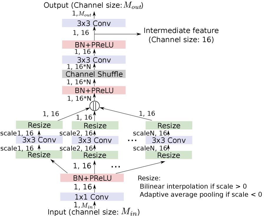
A diagram of the network architecture is shown in Fig. 7. Our network is based on ESPNetv2 [16], a computationally efficient semantic segmentation network. It consists of modules such as Extremely Efficient Spatial Pyramid (EESP), Efficient Point-Wise Convolution (EffPWConv), Efficient Pyramid Pooling (EffPyrPool). For detailed descriptions of those modules, we refer the readers to [16]. An auxiliary segmentation branch is attached to the middle of the main network of ESPNetv2 for estimating uncertainty used in the loss weighting [7].
7 Analysis of the prediction distributions
In Table 8 , we show the distributions of the predictions by each of the source models over the target classes conditioned on the source classes, as well as the target label ID of the maximum probability for each source class and the actual target label ID used in the label conversion to see the validity of the heuristic label mappings. The distributions are calculated using the labeled test images of Greenhouse A.
|
Sky |
Building |
Pole |
Road |
Pavement |
Tree |
Sign symbol |
Fence |
Car |
Pedestrian |
Bicyclist |
Road marking |
|
| 1 | 1.72 | 19.58 | 11.87 | 0.64 | 0.98 | 95.30 | 26.39 | 93.07 | 0.00 | 0.00 | 36.00 | 28.63 |
| 2 | 92.01 | 80.00 | 71.27 | 38.33 | 37.80 | 4.70 | 73.61 | 6.93 | 80.98 | 98.25 | 61.33 | 59.29 |
| 3 | 6.27 | 0.42 | 16.87 | 61.03 | 61.23 | 0.00 | 0.00 | 0.00 | 19.02 | 1.75 | 2.67 | 12.09 |
| max | 2 | 2 | 2 | 3 | 3 | 1 | 2 | 1 | 2 | 2 | 2 | 2 |
| 4 | 2 | 2 | 3 | 3 | 1 | 2 | 2 | 2 | 4 | 4 | 2 |
| Road | Sidewalk | Building | Wall | Fence | Pole | Traffic light | Traffic sign | Vegetation | Terrain | Sky | Person | Rider | Car | Truck | Bus | Train | Motorcycle | Bicycle | |
| 1 | 0.00 | 6.19 | 0.54 | 0.00 | 4.55 | 1.18 | 0.00 | 0.00 | 83.02 | 0.00 | 0.00 | 0.00 | 0.00 | 0.00 | 0.00 | 0.00 | 0.00 | 0.00 | 28.81 |
| 2 | 54.28 | 21.12 | 99.46 | 0.00 | 90.00 | 81.25 | 0.00 | 0.00 | 16.76 | 0.00 | 0.00 | 100.0 | 0.00 | 85.64 | 0.00 | 100.0 | 0.00 | 0.00 | 69.49 |
| 3 | 45.72 | 72.69 | 0.00 | 0.00 | 5.45 | 17.57 | 0.00 | 0.00 | 0.22 | 0.00 | 0.00 | 0.00 | 0.00 | 14.36 | 0.00 | 0.00 | 0.00 | 0.00 | 1.69 |
| max | 2 | 3 | 2 | - | 2 | 2 | - | - | 1 | - | - | 2 | - | 2 | - | 2 | - | - | 2 |
| 3 | 3 | 2 | 2 | 2 | 2 | 2 | 2 | 1 | 3 | 4 | 4 | 4 | 2 | 2 | 2 | 2 | 2 | 2 |
|
Road |
Grass |
Tree |
Sky |
Obstacle |
|
| 1 | 1.15 | 48.73 | 43.63 | 0.09 | 0.00 |
| 2 | 18.83 | 28.54 | 50.06 | 96.63 | 0.00 |
| 3 | 80.02 | 22.72 | 6.30 | 3.28 | 0.00 |
| max | 3 | 1 | 2 | 2 | - |
| 3 | 1 | 1 | 4 | 2 |
In the majority of the source classes, the target label of the maximum probability is the same as the one assigned heuristically. “Fence” in CamVid, “Road” in Cityscapes, and “Tree” in Freiburg Forest were assigned a target label different from the one with the maximum probability. In the model trained with Cityscapes, some source classes did not appear in the prediction on the target images.
Note that these distributions are calculated with the ground truth labels of the target images, which we do not expect to have in real environments, and thus this information is unable. In practice, as we show in the experiments, the definition of the mappings based on the heuristics resulted in good performances.
8 Policy of manual annotation on the test images
For the evaluation of our method, we created test datasets for Greenhouse A, B, and C with manually annotated labels. All annotation was done by the first author, who did not have specific experience of pixel-level annotation on image datasets.
We adopted coarse annotation to reduce the time of manual annotation. For example, small regions of objects other than plants that can be seen through the plant rows are annotated as plants, rather than the object classes that the regions actually belong to. The aim our method is to train the model for scene recognition in robot navigation to identify the object class of the regions in an image, especially regions of plants covering the paths, and to make a decision whether to traverse the object based on the object class. For this purpose, we suppose that pixel-level precision is not necessary. The model should rather be able to recognize the presence of plant etc. We, therefore, gave region-wise annotation rather than labels with pixel-level precision, so that the ability of recognizing the object class of image regions can be evaluated.
9 Qualitative evaluation on Greenhouse B and C
Fig. 8 and 9 show the qualitative results of the adaptation to Greenhouse B and C, respectively. Similar to the results on Greenhouse A shown in 4.2, more smooth and noise-less segmentation is achieved by the proposed method.


10 Implementation details of the baseline methods
10.1 Description of the feature for SP-SVM
We used the SVM model implemented in scikit-learn library [43]. The Radial Basis Function (RBF) kernel was used with the default parameters and one-versus-one decision function was chosen. For superpixel generation, we used a method by Felzenszwalb et al. [44] implemented in scikit-image library [45].
The feature design we adopt is based on the one used in a paper [46]. It consists of color features and texture features. The color features are mean RGB and HSV values, histograms of hue and saturation values. The texture features are calculated via applying filters in LM filter bank [47]. The filter responses are summarized by averaging and taking maximum within the superpixel and concatenated. In addition to the original feature design in [46], we added location features which are mean of and coordinates to exploit the spatial information.
| Type | Description | Dim. |
|---|---|---|
| RGB value | RGB mean | 3 |
| HSV value | RGB mean in HSV color space | 3 |
| Hue | Histogram of hue | 8 |
| Saturation | Histogram of saturation | 5 |
| LM average | Average filter responses from LM filter set | 18 |
| LM Maximum | Histogram of maximum filter responses | 18 |
| Location | Mean x / y coordinate values normalized by the image width / height | 2 |
| Total number of dimension | 57 |
10.2 Training details of the UDA baselines
10.2.1 Network architecture
DeepLab v2 [48] with ResNet101 backbone [12] is used as the semantic segmentation model in the original work of all the baseline methods of UDA. Although it is different from our model, we also adopt DeepLab v2 in the baselines to keep their implementation as much as possible. CRST and ProDA are trained on an NVIDIA Quadro RTX 8000, and Seg-Uncertainty is trained on an NVIDIA GeForce 1080Ti with 11GB memory.
10.2.2 CRST
In CRST [34], the source models are pre-trained by supervised training and we follow the implementation. We first train a model with a source dataset with its original label set for 200 epochs. We then replace the final classification layer with -class classifier where denotes the number of object classes in the target dataset. The model with the replaced classifier is fine-tuned with the source labels converted to the target label set defined in Table 1 for 50 epochs. Initial learning rate is for the final classification layer and for the rest of the layers. The polynomial learning rate scheduling [49] is used with the power of 0.9. Other hyper-parameters are unchanged from their source code.
10.2.3 Seg-Uncertainty
10.2.4 ProDA
ProDA [8] follows the same warm-up strategy as Seg-Uncertainty. We, therefore, use the same warm-up models trained in Seg-Uncertainty in ProDA. Although ProDA and Seg-Uncertainty both use DeepLabv2 as a segmentation network, the architecture of the segmentation networks is slightly different between Seg-Uncertainty and ProDA, such as the number of channels of the intermediate feature map. We modified the source code of ProDA to adjust to the network. Other hyper-parameters are unchanged from their source code.
11 Results of the baseline methods
11.1 Qualitative evaluation of the UDA methods
Fig. 10 shows qualitative results of the UDA baseline methods on Greenhouse A dataset. As shown quantitatively in 4.3, the proposed method (CV+CS+FR) outperformed the baseline methods, especially Seg-Uncertainty [7] and ProDA [8]. In the segmentation results of Seg-Uncertainty and ProDA, a large part of the bottom of the images are wrongly classified as ground regions. This is similar to the structural feature of the images in CS. This tendency was possibly enhanced by the adversarial learning on the output layer employed in the first stage of those methods.
Compared to Seg-Uncertainty and ProDA, CRST [34] produced better segmentation results. CRST chooses pseudo-labels simply based on the confidence of the predictions, and resulting pseudo-labels are sparse. In other words, CRST conservatively generates pseudo-labels with only confidently predicted labels. As a result, the performance was better than the other two baselines. Our proposed method also generates pseudo-labels in a conservative way via multiple model’s agreement. It may imply that it is a better approach to generate pseudo-labels in a conservative way when the source and the target have a large structural difference. The proposed method provides a natural way of doing so without relying on a specific dataset, which allows for avoiding biased training.


11.2 Effect of GAN-based image style transfer
We trained the CycleGANs using CS and FR as source datasets and Greenhouse A as a target dataset. It is the first step of MADAN [37], a multi-source UDA method for semantic segmentation. For each source dataset, we trained a CycleGAN for 200 epochs.
Fig. 11 shows the results of image style transfer between CS/FR and Greenhouse A datasets. The style transfer resulted in inconsistency of image contents, e.g., the ground region in Fig. 11 is transferred to green plant-like objects in Fig. 11, and the bottom part of the plant row and a large part of an artificial object on the right in Fig. 11 are transferred to ground in Fig. 11. Similarly, plants on the right in Fig. 11 are transferred to gray objects like a wall in Fig. 11, and some plant parts in Fig. 11 are mapped to sky in 11.
This may be due to the large domain shift that stems from the structural differences of the environments.
Although MADAN further employs training procedures to aggregate the data from multiple domains closer to each other with constraints on the semantic consistency [37], the inconsistency of the style transfer in the first step shown above will affect the adaptation performance.