Multi-twist polarization ribbon topologies in highly-confined optical fields

Since the inception of electromagnetic theory, the polarization of light, i.e. the oscillation direction of the electric field vector, has been a central concept to our understanding of optics, giving rise to countless applications [1]. For plane waves and in paraxial beams, the polarization has been recognized as a transverse quantity and, hence, it can be represented by a set of two orthogonal basis vectors. For instance, in the linear and circular bases, the polarization of an optical beam can be represented by superpositions of linearly horizontally and linearly vertically, or circularly-left and circularly-right polarized beams, respectively. The ratio and the relative phase between the two polarization components define the oscillations of the electric field vector’s tip upon propagation or in time, and its trajectory in the plane transverse to its propagation direction, typically given by an ellipse [1]. This description of the light field by a so-called polarization ellipse at each point in space is even valid in highly confined fields exhibiting out-of-plane field components, as long as the field itself is monochromatic. In two different cases, this ellipse becomes singular [2, 3, 4]: (i) the ellipse’s major and minor axes are undefined, resulting in circular polarization (C-point); (ii) the minor axis of the ellipse is zero and its surface normal is undefined, and thus the polarization is linear (L-line). These so-called polarization singularities in general arise in light fields with spatially inhomogeneous polarization distributions, which we refer to as space-varying polarized light beams. They have recently received great attention owing to their peculiar optical features and applications [5, 6, 7]. Vector vortex beams [5] - space-varying linearly-polarized beams - and Poincaré beams [8] - optical beams containing all types of polarization - are among this class of spatially inhomogeneously polarized beams. These beams are interesting both at the fundamental and applied levels. For instance, they can be used to enhance measurement sensitivity [9, 10], to transport high-power in nonlinear media [11], or to generate exotic optical beams with peculiar topological structures [12, 13]. In particular, spatially structured light fields with field components along the propagation direction were predicted by Freund to show so-called optical polarization Möbius strips and twisted ribbons [14, 15], with the former recently confirmed experimentally in tightly focused fields [16] as well as the originally proposed scheme of crossing beams [17]. Here, we will experimentally demonstrate the generation and stability of the latter in highly confined fields, specifically looking at the dynamics of the twisted ribbon when propagating through the focal volume of a tailored space-varying polarized light beam.

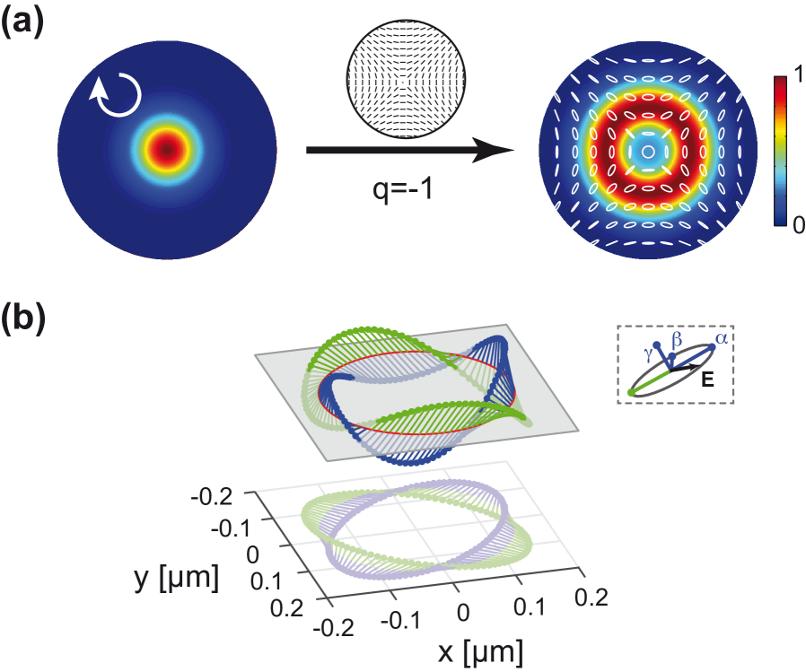
There are several different methods to generate optical beams possessing inhomogeneous polarization distributions in their transverse plane. For instance, phase-only spatial light modulators (SLMs) [18, 19, 20], non-unitary polarization transformation [21], and spatially structured birefringent plates [8, 22] have so far been used to generate Poincaré or vector vortex beams. In this article, we use the latter technique to generate full Poincaré beams [8] by means of a spatially structured liquid crystal device, referred to as $q$-plate [23]. The $q$-plate couples spin to orbital angular momentum, and thus allows for generating certain classes of space-varying optical beams when it is fed with an elliptically polarized input beam. Choosing a left-handed circularly polarized Gaussian beam, $\hat{\mathbf{e}}_{\text{L}}$, as input, the $q$-plate coherently transforms this field distribution into

$\displaystyle\mathbf{E}(\mathbf{r})\approx\left(\cos{\left(\frac{\delta}{2}\right)}\,E_{\text{L}}(\rho;z)\,\hat{\mathbf{e}}_{\text{L}}+i\sin{\left(\frac{\delta}{2}\right)}\,E_{\text{R}}(\rho;z)\,e^{2iq\phi}\,\hat{\mathbf{e}}_{\text{R}}\right),\!\!\!\!$

(1)

where $\delta$ is the chosen optical retardation of the $q$-plate, $\rho,\phi,z$ are cylindrical coordinates, $q$ is the $q$-plate’s topological charge, $\hat{\mathbf{e}}_{\text{L}}$ and $\hat{\mathbf{e}}_{\text{R}}$ are the left- and right-handed polarization unit vectors, and $E_{\text{L}}(\rho;z)$ and $E_{\text{R}}(\rho;z)$ are the beam profiles of the left- and right-handed circularly polarized beams, respectively [24]. The orientation of liquid crystal molecules in the transverse plane of a given $q$-plate with topological charge of $q=-1$ is shown in Fig. 1-(a). Adjusting the optical retardation $\delta$ of the plate changes the superposition ratio, and thus the polarization topology. For instance, when (i) $\delta=0,2\pi$, the plate won’t change the initial state of the beam and the beam polarization remains left-handed circular; (ii) $\delta=\pi$, the plate works as a structured half-wave plate and converts the Gaussian beam into a right-handed circularly polarized doughnut beam possessing orbital angular momentum of $2q$; (iii) $\delta=\pi/2$ the plate generates a coherent superposition of (i) and (ii). In the latter case (iii), the beam exhibits a point of circular polarization on the optical axis (C-point) and an azimuthal polarization structure with polarization topological charge of $\eta=q$. An example of such polarization topology is shown in Fig. 1-(a). Note that the polarization topology shown in Fig. 1-(a) corresponds to that resulting from a $q=-1$-plate. However, for practical reasons we use a $q=1$-plate followed by a half-wave plate in the experiment to mimic the $q=-1$-plate topology (see Fig. 2).

Upon tight focusing, strong (longitudinal) $z$-components of the incoming transversely polarized beam described by Eq. (1) emerge. Using vectorial diffraction theory [25], one can show that the total electric field at the focus will have the following form [26]

	$\displaystyle\mathbf{E}_{\text{focus}}(\mathbf{r})$	$\displaystyle=$	$\displaystyle\left(\widetilde{E}_{\text{L}}(\rho;z)\,\hat{\mathbf{e}}_{\text{L}}+\widetilde{E}_{\text{R}}(\rho;z)\,e^{2iq\phi}\,\hat{\mathbf{e}}_{\text{R}}\right)$		(2)
		$\displaystyle+$	$\displaystyle\left(\widetilde{E}^{z}_{\text{L}}(\rho;z)e^{i\phi}+\widetilde{E}^{z}_{\text{R}}(\rho;z)e^{i(2q-1)\phi}\right)\hat{\mathbf{e}}_{\text{z}},$		(4)

where $\widetilde{E}_{\text{L}}$ and $\widetilde{E}_{\text{R}}$ are the components of the transverse electric field (including the weight factors) at the focus, and $\widetilde{E}^{z}_{\text{L}}$ and $\widetilde{E}^{z}_{\text{R}}$ are the associated $z$-components. The exact form for these amplitudes, i.e. $\widetilde{E}_{\text{L}}$, $\widetilde{E}_{\text{R}}$, $\widetilde{E}^{z}_{\text{L}}$ and $\widetilde{E}^{z}_{\text{R}}$, can be found in [26]. The last term in Eq. (2) corresponds to spin-orbit coupling amplified by tight focusing with a high-numerical aperture lens, which renders the polarization vector in 3-dimensional space, with its amplitude depending on the numerical aperture (NA) of the focusing lens. However, the polarization ellipse traced by the tip of the electric field vector in time remains in a 2-dimensional plane for any given point in space. Nevertheless, the spatial distribution of the polarization ellipse forms a specific topology in 3-dimensional space, which is dictated by the topological charge of the $q$-plate. Without loss of generality, we consider a radial position $\rho=\rho_{0}$ where the amplitude of the contributions of the initial right- and left-circular polarization components to the longitudinal focal field component are equal, i.e. $\widetilde{E}^{z}_{\text{L}}(\rho_{0})=\widetilde{E}^{z}_{\text{R}}(\rho_{0})$. The $z$-component of the electric field, apart from a phase $\exp{(iq\phi)}$, will now be proportional to $\cos\left[(q-1)\phi\right]$. The electric field intensity of the $z$-component will then be proportional to $\left|\cos\left[(q-1)\phi\right]\right|^{2}$, which results in a $2\left|q-1\right|$-fold symmetry. This z-component of the electric field turns the 2-dimensional into a 3-dimensional polarization topology. The structure of the polarization topology can be studied by evaluating the spatial dependence of either the major or minor axes of the polarization ellipse. Tracing the focal field on a closed loop around the on-axis C-point, the major axis of the polarization ellipse oscillates $|q-1|$ times through the transverse plane. In the 3-dimensional perspective, the major (or the minor) axis of the polarization ellipse, depending on the value of $q$, forms a Möbius or a ribbon topology with $|q-1|$ twists. While the existence of polarization Möbius strips with 3/2-twists and 5/2-twists, for the case of $q=-1/2$ and $-3/2$, respectively, has been experimentally demonstrated recently [16], we here will look at the case of ribbons with integer twists for integer values of $q$.

To determine the polarization ellipse, and consequently its major and minor axes in three dimensions, it is necessary to measure amplitude and phase of the full complex vectorial light field in the plane of observation. This can be achieved by employing a probe as a local field sensor and utilizing the angularly resolved far-field scattering by this probe while point-wise scanning the latter relative to the field distribution. This technique, named Mie-scattering nano-interferometry (see [27] for more details on the technique), was shown to achieve deep sub-wavelength spatial resolution in the experimental study of vectorial focal fields. The Mie-scattering nano-interferometry has previously allowed for the experimental verification of optical polarization Möbius strips in both, tailored light fields [16] and in the focal region of a tightly focused linearly polarized beam around points of transversely spinning fields [28]. The general experimental concept will be discussed in the following, while details are discussed in [27].

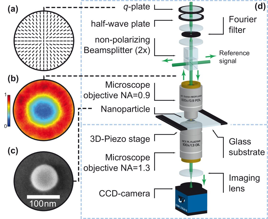
The custom-built experimental setup is shown in Fig. 2 [27]. As a nano-probe, a single gold sphere with a transverse diameter of $d=80~\text{nm}$ and a height of $h=86~\text{nm}$ (see scanning electron micrograph in Fig. 2-(c)) on a glass substrate is utilized. For the measurement, it is moved through the investigated field distribution via a 3-dimensional piezo stage. The angularly resolved detection of the interference between the light scattered by the probe into the lower half-space forward direction and the directly transmitted light in this region is realized by collecting the light via an oil-immersion microscope objective ($\text{NA}=1.3$) and imaging its back focal plane onto a CCD camera (see Fig. 2-(d)). This interferometric information for each position of the probe relative to the investigated field is equivalent to an observation of the scattering process from various directions. Thus, it allows for a retrieval of the relative phase information of the distributions under study from the far-field [27]. The highly confined field distribution containing a twisted ribbon formed by tracing the major axis of the polarization ellipse along a closed loop around the optical axis is created in the shown setup by sending an initially right-handed circularly polarized Gaussian beam onto a $q=1$-plate [23] (see sketch of its structure in Fig. 2-(a)) and a subsequent half-wave plate.

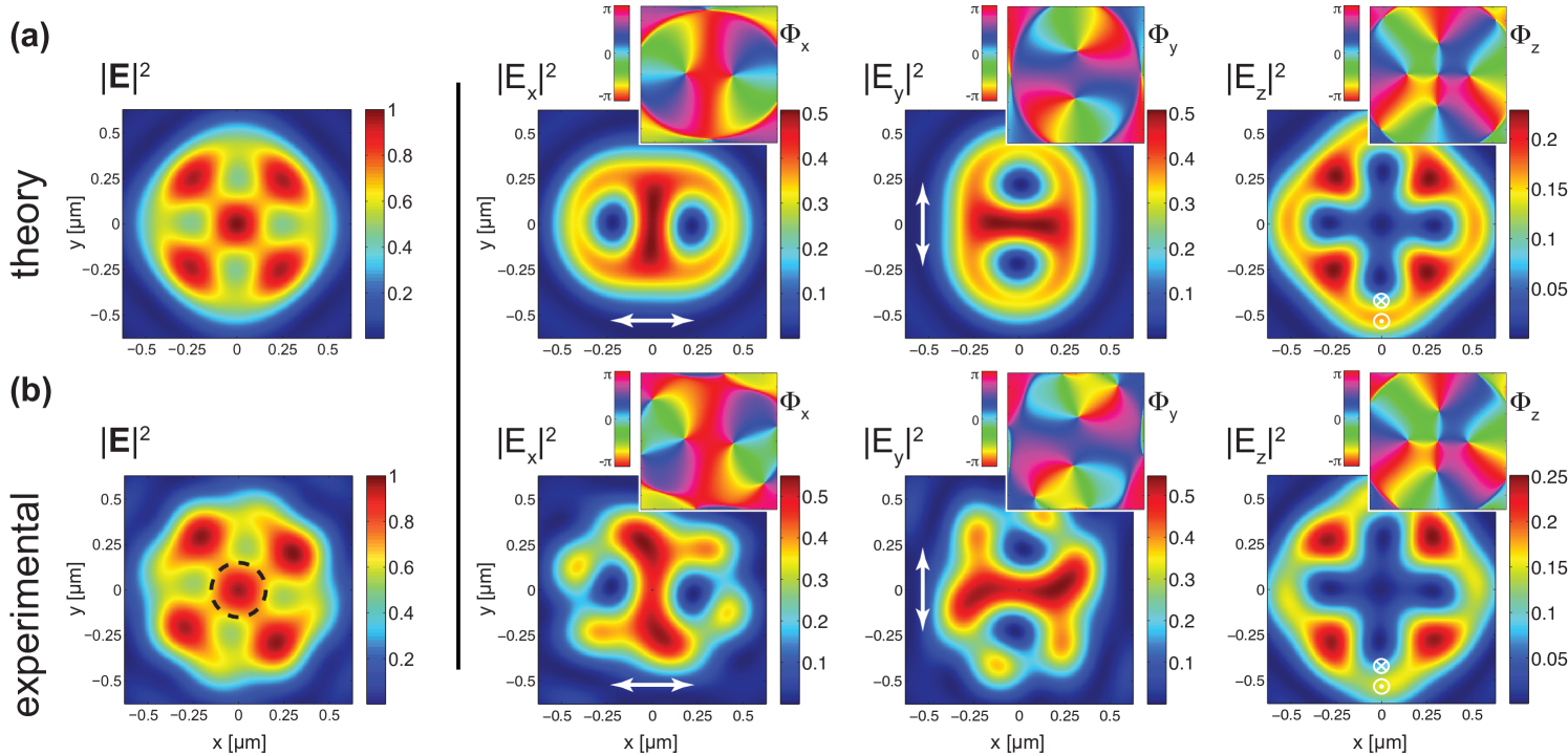
As discussed in the previous section, this combination results effectively in the operation of a $q=-1$-plate. By adjusting the voltage applied to the liquid-crystal-based $q$-plate [24, 29], a coaxial superposition of the initial right-handed circular polarized Gaussian beam ($\text{HyGG}_{0,0}(\rho,\phi,z)\,\hat{\mathbf{e}}_{\text{R}}$) and a left-handed circularly polarized hypergeometric Gauss beam ($\text{HyGG}_{-2,2}(\rho,\phi,z)\,\hat{\mathbf{e}}_{\text{L}}$) is generated [30, 31] with the Hypergeometric Gauss modes $\text{HyGG}_{p,\ell}(\rho,\phi,z)$ having the radial and azimuthal indices of $p$ and $\ell$, respectively. The resulting full Poincaré beam [8, 24] is filtered spatially with a pinhole to obtain the lowest radial order of both constituting beams in the Laguerre Gauss basis, i.e. $\text{LG}_{0,0}(\rho,\phi,z)\,\hat{\mathbf{e}}_{\text{R}}$ and $\text{LG}_{0,2}(\rho,\phi,z)\,\hat{\mathbf{e}}_{\text{L}}$ (see Fig. 2-(b) for the experimentally achieved intensity distribution). The spatially filtered beam is then transmitted through two orthogonally oriented non-polarizing beamsplitters to redirect part of the incoming beam and the light reflected from the sample onto corresponding photodetectors. By using two orthogonally aligned beamsplitters, the remaining weak polarizing effect of non-polarizing beamsplitters can be compensated for. Finally, the generated beam is focused by a microscope objective with an NA of $0.9$, resulting in the complex focal field distribution under study, shown in Fig. 3-(a).

Scanning the described nano-probe through this focal field and applying the reconstruction algorithm [27] to the collected far-field intensity information results in the experimentally reconstructed focal field distributions shown in Fig. 3-(b). Here, the excitation wavelength was chosen to be $\lambda=530~\text{nm}$, with an experimentally determined relative permittivity of the utilized nano-probe of $\epsilon=-3.1+2.5\,i$. The total electric energy density (depicted on the left side of Fig. 3-(b)) strongly resembles the numerically simulated field distributions calculated via vectorial diffraction theory (Fig. 3-(a)) [25, 32]. The energy density distributions of the individual electric field components (right side of Fig. 3-(b)) show minor deviations specifically in the transverse field components. The resulting phase distributions are also shown as insets. The phase distribution of the transverse components of the electric field at the focus exhibit two singularities of topological charge $\pm 1$, both displaced (vertically or horizontally) away from the optical axis. Due to spin-orbit coupling, the $z$-component of the electric field under tight focusing gains extra phase singularity points, in this case five singular points that are shown in Fig. 3. The $z$-component of the electric field now reaches amplitudes comparable to that of the transverse components (see the scale bar in Fig. 3-(b)), and thus breaks the cylindrical symmetry into a four-fold symmetric pattern.

The major and minor semi-axes of the polarization ellipse $\boldsymbol{\alpha}(\mathbf{r}),\boldsymbol{\beta}(\mathbf{r})$ as well as the normal to the polarization ellipse $\boldsymbol{\gamma}(\mathbf{r})$ for the electric field $\mathbf{E}$ at any point of $\mathbf{r}$ can be calculated by [3, 33]

$\displaystyle\begin{array}[]{l}\boldsymbol{\alpha}(\mathbf{r})=\frac{1}{\left|\sqrt{\mathbf{E}\cdot\mathbf{E}}\right|}\,\Re\left(\mathbf{E}\sqrt{\mathbf{E}^{*}\cdot\mathbf{E}^{*}}\right),\cr\boldsymbol{\beta}(\mathbf{r})=\frac{1}{\left|\sqrt{\mathbf{E}\cdot\mathbf{E}}\right|}\,\Im\left(\mathbf{E}\sqrt{\mathbf{E}^{*}\cdot\mathbf{E}^{*}}\right)\cr\boldsymbol{\gamma}(\mathbf{r})=\Im\left(\mathbf{E}^{*}\times\mathbf{E}\right),\end{array},$

(8)

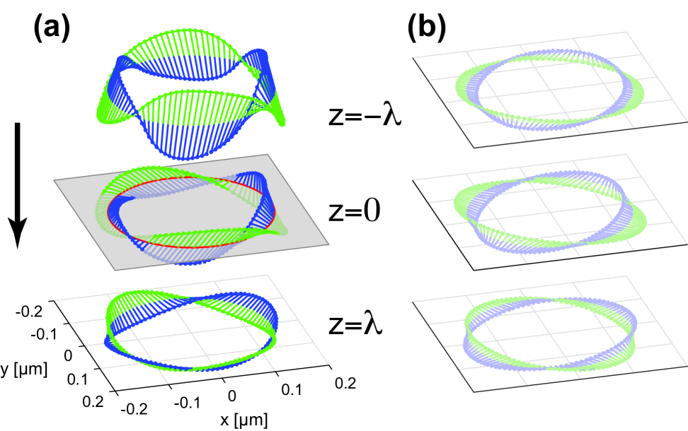
where $\Re(u)$, $\Im(u)$ and $u^{*}$ represent the real and imaginary parts of $u$, and its complex conjugate, respectively. With these equations, we calculated the local polarization ellipse in the focal plane, $z=0$, from the experimental field data at each point on a circular trace with radius $\rho=150~\text{nm}$ around the optical axis (shown in Fig. 3-(b) as a black dashed circle). The major axes of the polarization ellipses for these points in 3-dimensional space are shown in the central row of Fig. 4. In order to see the 3-dimensional topological structure, the semi-axes are coloured in blue and green, revealing a twisted ribbon with twist index $-2$. Note that the number of twists is given by $|q-1|$, which for the above case is $|-1-1|=2$ (the minus sign indicates that the direction of the twists is clockwise). The projection of the major axis onto the transverse plane is shown next to the ribbon in Fig. 4-(b). Following the major axes of the ellipses around the C-point also shows the 2-dimensional polarization topology with the polarization topological index of $-1$ in the transverse plane. We observe the same 3-dimensional (ribbon with two twists) and 2-dimensional (polarization topological index of $-1$) topologies for different radii around the C-point (not shown here). However, for radii, $\rho\gg 500$ nm, the field amplitudes drop quickly due to the strong spatial confinement of the focal field, resulting in a low signal-to-noise ratio.

In a next step, we also studied the behavior of the observed ribbon topology in other planes parallel to the focal plane within the focal volume. In order to observe the evolution of the 3-dimensional polarization topology, we retrieve the electric field components and their relative phases one wavelength before and after the focus, i.e. $z=\pm\lambda=\pm 530~\text{nm}$ from the reconstructed focal data. Again, the major axes of the polarization ellipses are retrieved for a given radius, i.e. $\rho=150~\text{nm}$, and plotted in 3-dimensional space. Figure 4 shows the evolution of the major axes of the polarization ellipses upon free-space propagation when it passes through the focal plane. The 3-dimensional polarization topology, i.e. ribbon with $-2$ twists, as well as the 2-dimensional polarization topology, shown in Fig. 4-(b) as a projection onto the corresponding planes, are conserved upon propagation through the focus. However, two main effects can be observed. First, the magnitude of the $z$-component of electric field is weaker outside the focal plane. Second, the topological structure rotates while traversing the focal plane. The latter effect is more visible in the projection shown in Fig. 4-(b) as 2-dimensional topology, and was previously observed for the 2-dimensional case [24]. Such a rotation in the 3-dimensional and 2-dimensional polarization topologies is caused by the difference in Gouy phases for $\text{LG}_{0,0}(\rho,\phi,z)$ and $\text{LG}_{0,-2}(\rho,\phi,z)$ beams. This propagation distance-dependent phase equals $-(2p+|\ell|+1)\arctan{(z/z_{R})}$ for $\text{LG}_{p,\ell}(\rho,\phi,z)$, where $z_{R}$ is the Rayleigh range. Thus, one expects a relative accumulated phase when propagating from $-z$ to the focal plane (with $|z|>>z_{R}$), and, hence, a rotation of $\pi/2$ of the polarization topology.

In summary, we studied the topological structure of an optical beam possessing a transverse polarization topological charge of $-1$ in the tight focusing regime. When such a structured beam is tightly focused, the longitudinal component of the electric field is enhanced, and the polarization structure forms a 3-dimensional topology. We utilized a recently introduced nanoscopic field reconstruction technique to measure all three components of the electric field as well as their relative phases. Calculating the major axes of the polarization ellipses from the measured data in 3-dimensional space reveals a ribbon-type topology with two twists when following a circular trace around the optical axis. We also observed the evolution of the multi-twisted polarization ribbon upon propagation through the focus.

This work was supported by the European Union’s Horizon 2020 Research and Innovation Programme (Q-SORT), grant number 766970. L. M. and E. S. acknowledge financial support from the European Union Horizon 2020 program, within the European Research Council (ERC) Grant No. 694683, PHOSPhOR. F. B., R. W. B. and E. K. acknowledge the support of Canada Research Chairs (CRC) program, and Natural Sciences and Engineering Research Council of Canada (NSERC).

References

- [1] Born M and Wolf E 2013 Principles of Optics: Electromagnetic Theory of Propagation, Interference and Diffraction of Light (Elsevier)
- [2] Nye J 1983 Proceedings of the Royal Society of London. A. Mathematical and Physical Sciences 387 105–132
- [3] Berry M 2004 Journal of Optics A: Pure and Applied Optics 6 675
- [4] Nye J F and Hajnal J 1987 Proc. R. Soc. Lond. A 409 21–36
- [5] Zhan Q 2009 Advances in Optics and Photonics 1 1–57
- [6] Rubinsztein-Dunlop H, Forbes A, Berry M, Dennis M, Andrews D L, Mansuripur M, Denz C, Alpmann C, Banzer P, Bauer T et al. 2016 Journal of Optics 19 013001
- [7] Aiello A, Banzer P, Neugebauer M and Leuchs G 2015 Nature Photonics 9 789
- [8] Beckley A M, Brown T G and Alonso M A 2010 Optics Express 18 10777–10785
- [9] D’ambrosio V, Spagnolo N, Del Re L, Slussarenko S, Li Y, Kwek L C, Marrucci L, Walborn S P, Aolita L and Sciarrino F 2013 Nature Communications 4
- [10] Berg-Johansen S, Töppel F, Stiller B, Banzer P, Ornigotti M, Giacobino E, Leuchs G, Aiello A and Marquardt C 2015 Optica 2 864–868
- [11] Bouchard F, Larocque H, Yao A M, Travis C, De Leon I, Rubano A, Karimi E, Oppo G L and Boyd R W 2016 Physical Review Letters 117 233903
- [12] Otte E, Alpmann C and Denz C 2016 Journal of Optics 18 074012
- [13] Larocque H, Sugic D, Mortimer D, Taylor A J, Fickler R, Boyd R W, Dennis M R and Karimi E 2018 Nature Physics 14, 1079
- [14] Freund I 2005 Optics Communications 249 7–22
- [15] Freund I 2010 Optics Letters 35 148–150
- [16] Bauer T, Banzer P, Karimi E, Orlov S, Rubano A, Marrucci L, Santamato E, Boyd R W and Leuchs G 2015 Science 347 964–966
- [17] Galvez E J, Dutta I, Beach K, Zeosky J J, Jones J A and Khajavi B 2017 Scientific Reports 7 13653
- [18] Maurer C, Jesacher A, Fürhapter S, Bernet S and Ritsch-Marte M 2007 New Journal of Physics 9 78
- [19] Galvez E J, Khadka S, Schubert W H and Nomoto S 2012 Applied Optics 51 2925–2934
- [20] Han W, Yang Y, Cheng W and Zhan, Q 2013 Optics Express 21 20692
- [21] Sit A, Giner L, Karimi E and Lundeen J S 2017 Journal of Optics 19 094003
- [22] Cardano F, Karimi E, Slussarenko S, Marrucci L, de Lisio C and Santamato E 2012 Applied Optics 51 C1–C6
- [23] Marrucci L, Manzo C and Paparo D 2006 Physical Review Letters 96 163905
- [24] Cardano F, Karimi E, Marrucci L, de Lisio C and Santamato E 2013 Optics Express 21 8815–8820
- [25] Richards B and Wolf E 1959 Proceedings of the Royal Society of London. Series A. Mathematical and Physical Sciences 253 358–379
- [26] Bliokh K Y, Ostrovskaya E A, Alonso M A, Rodríguez-Herrera O G, Lara D and Dainty C 2011 Optics Express 19 26132–26149
- [27] Bauer T, Orlov S, Peschel U, Banzer P and Leuchs G 2014 Nature Photonics 8 23–27
- [28] Bauer T, Neugebauer M, Leuchs G and Banzer P 2016 Physical Review Letters 117 013601
- [29] Larocque H, Gagnon-Bischoff J, Bouchard F, Fickler R, Upham J, Boyd R W and Karimi E 2016 Journal of Optics 18 124002
- [30] Karimi E, Piccirillo B, Marrucci L and Santamato E 2009 Optics Letters 34 1225–1227
- [31] Karimi E, Zito G, Piccirillo B, Marrucci L and Santamato E 2007 Optics Letters 32 3053–3055
- [32] Novotny L and Stranick S J 2006 Annu. Rev. Phys. Chem. 57 303–331
- [33] Dennis M 2002 Optics Communications 213 201–221
- [34] Zhao Y, Edgar J S, Jeffries G D, McGloin D and Chiu D T 2007 Physical Review Letters 99 073901