Multi-view Self-supervised Disentanglement for General Image Denoising
Abstract
With its significant performance improvements, the deep learning paradigm has become a standard tool for modern image denoisers. While promising performance has been shown on seen noise distributions, existing approaches often suffer from generalisation to unseen noise types or general and real noise. It is understandable as the model is designed to learn paired mapping (e.g. from a noisy image to its clean version). In this paper, we instead propose to learn to disentangle the noisy image, under the intuitive assumption that different corrupted versions of the same clean image share a common latent space. A self-supervised learning framework is proposed to achieve the goal, without looking at the latent clean image. By taking two different corrupted versions of the same image as input, the proposed Multi-view Self-supervised Disentanglement (MeD) approach learns to disentangle the latent clean features from the corruptions and recover the clean image consequently. Extensive experimental analysis on both synthetic and real noise shows the superiority of the proposed method over prior self-supervised approaches, especially on unseen novel noise types. On real noise, the proposed method even outperforms its supervised counterparts by over 3 dB.
††footnotetext: ∗Equal contribution.
1 Introduction
Image restoration is a critical sub-field of computer vision, exploring the reconstruction of image signals from corrupted observations. Examples of such ill-posed low-level image restoration problems include image denoising [41, 32, 19, 28, 29, 37, 45], super-resolution [10, 22, 3, 44, 33], and JPEG artefact removal [9, 14, 34], to name a few. Usually, a mapping function dedicated to the training data distribution is learned between the corrupted and clean images to address the problem. While many image restoration systems perform well when evaluated over the same corruption distribution that they have seen, they are often required to be deployed in settings where the environment is unknown and off the training distribution. These settings, such as medical imaging, computational lithography, and remote sensing, require image restoration methods that can handle complex and unknown corruptions. Moreover, in many real-world image-denoising tasks, ground truth images are unavailable, introducing additional challenges.
Limitations of existing methods:
Current low-level corruption removal tasks aim to address the inquiry of “what is the clean image provided a corrupted observation?” However, the ill-posed nature of this problem formulation poses a significant challenge in obtaining a unique resolution [6].
To mitigate this limitation, researchers often introduce additional information, either explicitly or implicitly. For example, in [18], Laine et al. explicitly use the prior knowledge of noise as complementary input, generating a new invertible image model. Alternatively, Learning Invariant Representation (LIR) [11] implicitly enforces the interpretability in the feature space to guarantee the admissibility of the output. However, these additional forms of information may not always be practical in real-world scenarios or may not result in satisfactory performance.
Main idea and problem formulation:
Our motivation for tackling this ill-posed nature stems from the solution in the 3D reconstruction of utilising multiple views to provide a unique estimation of the real scene [1]. Building on this motivation, we propose a training scheme that is explicitly built on multi-corrupted views and perform Multi-view self-supervised Disentanglement, abbreviated as MeD.
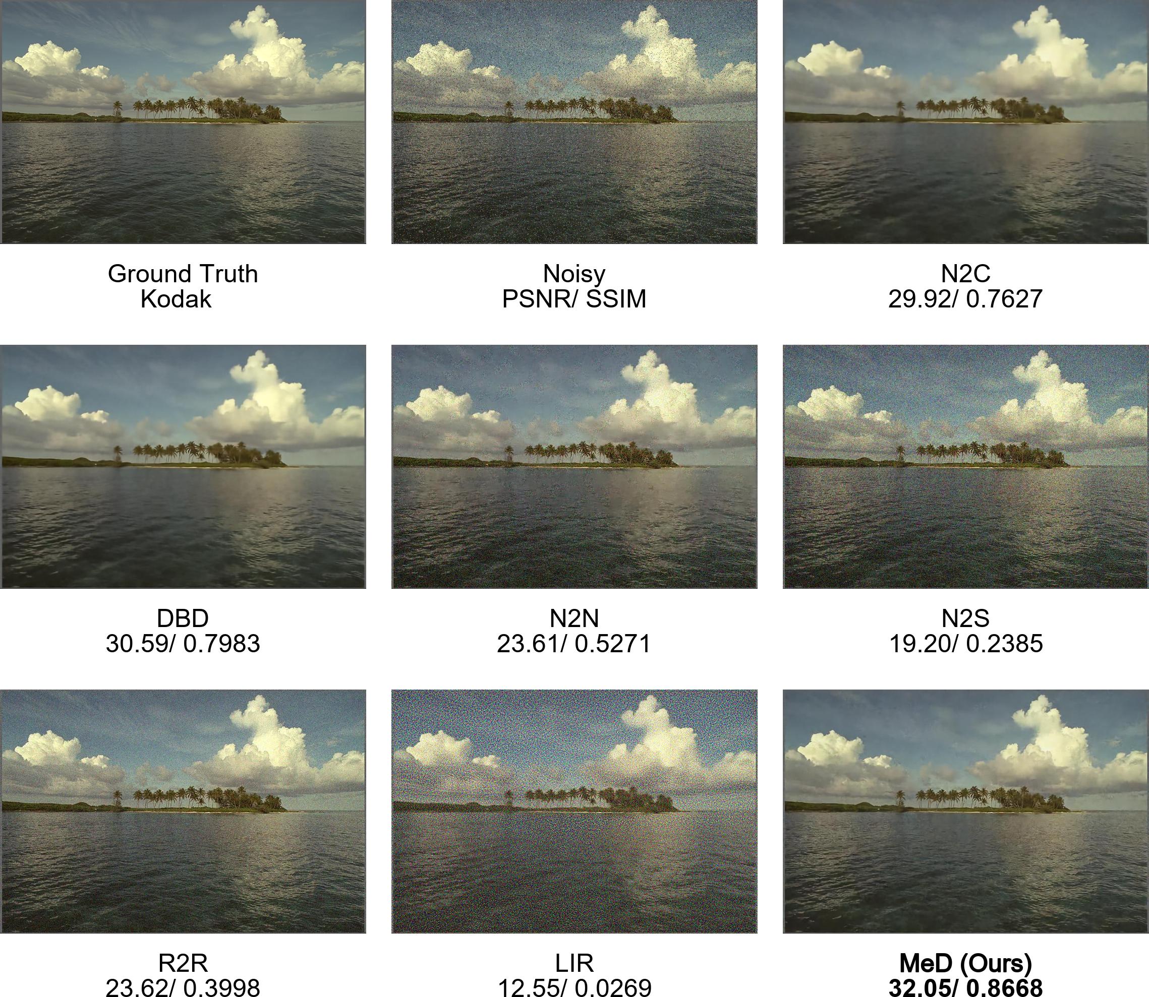
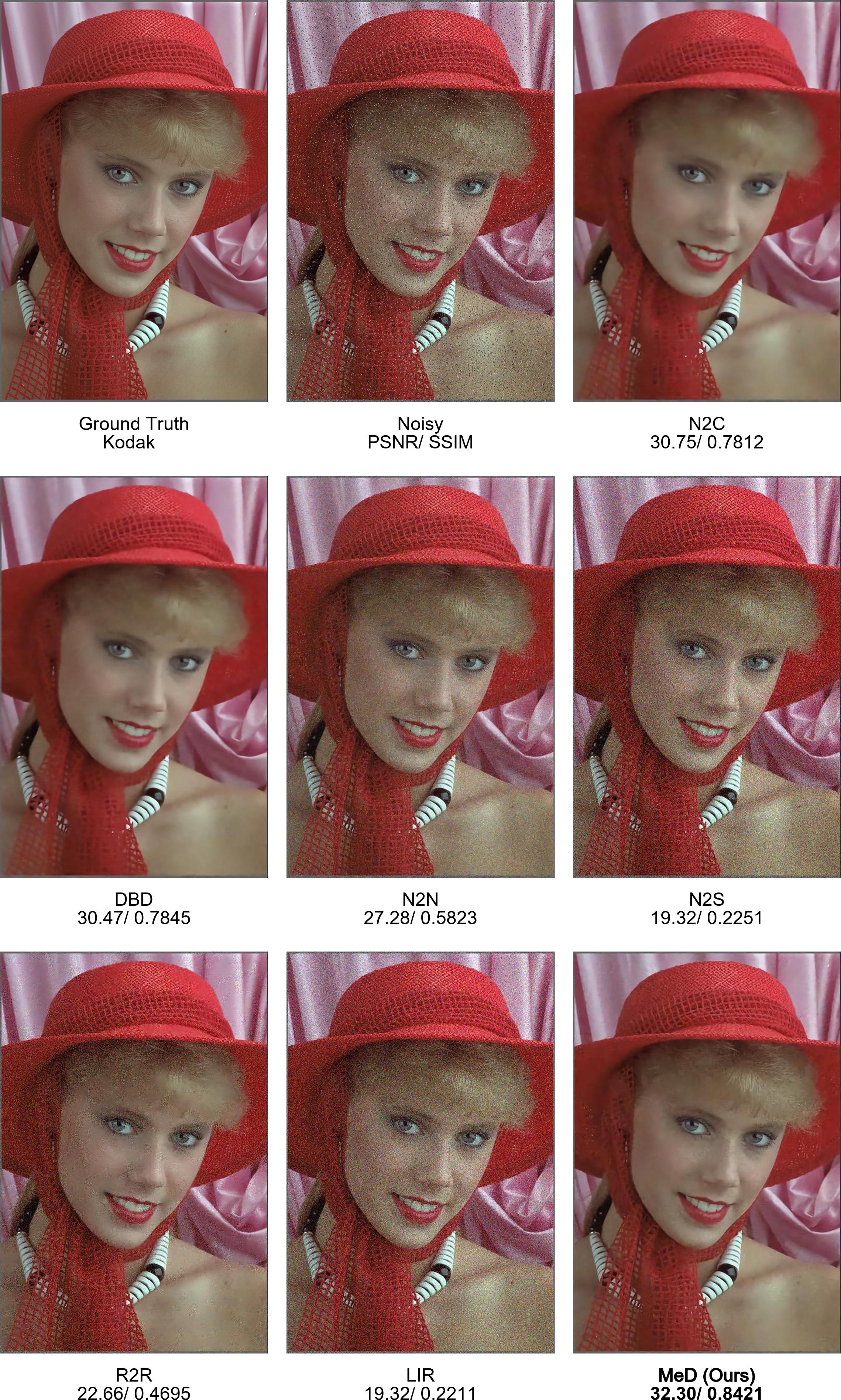
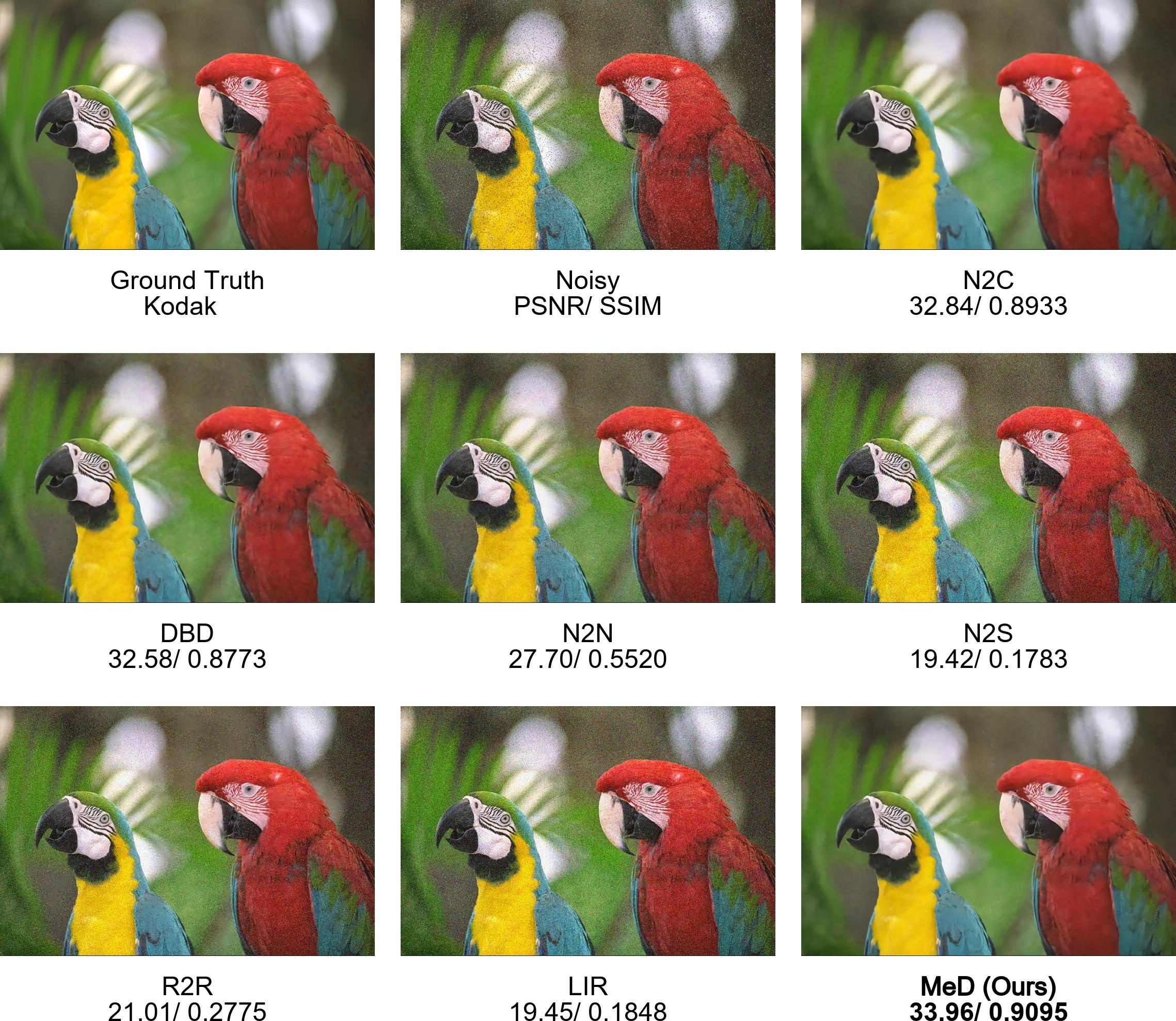
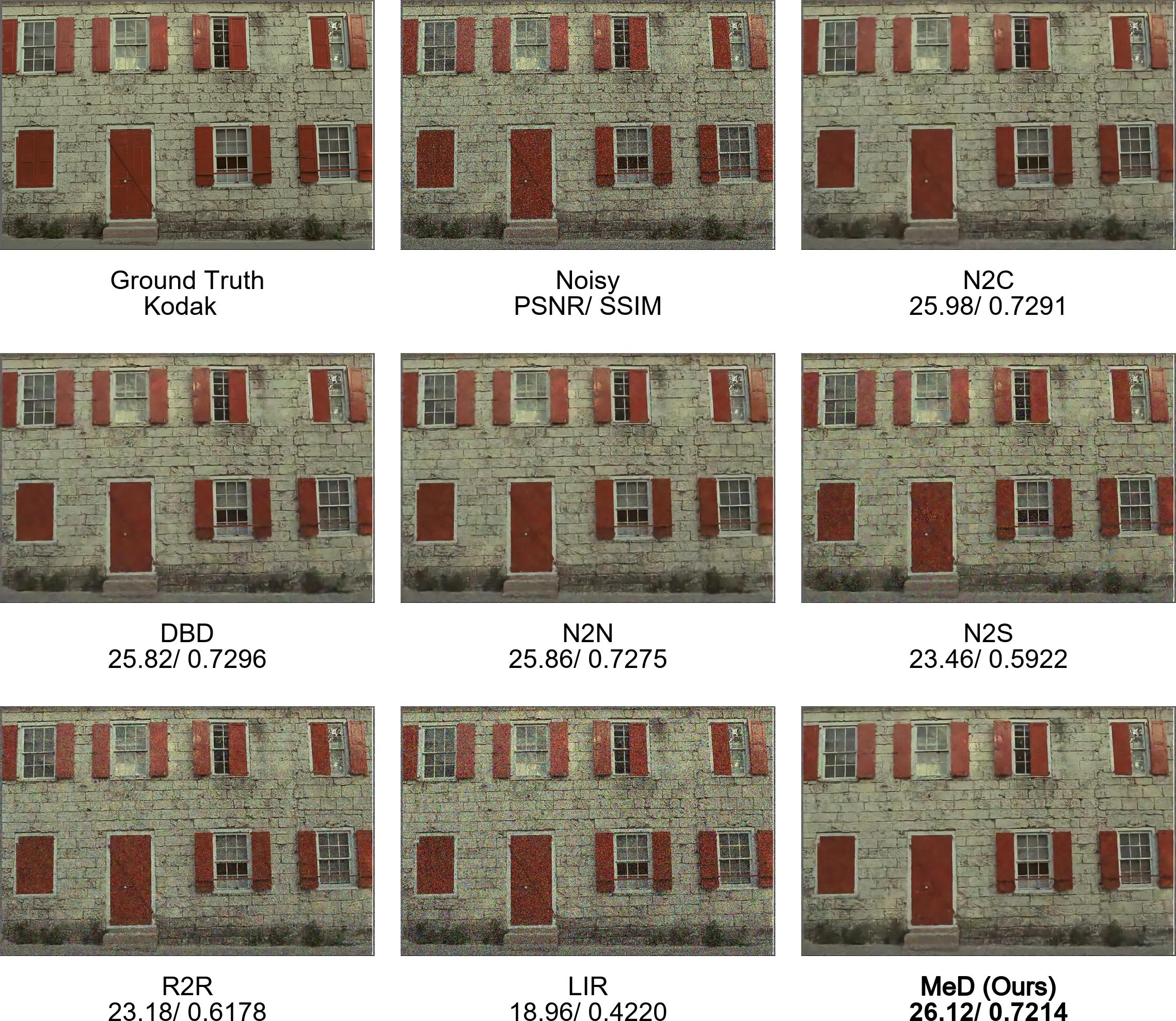
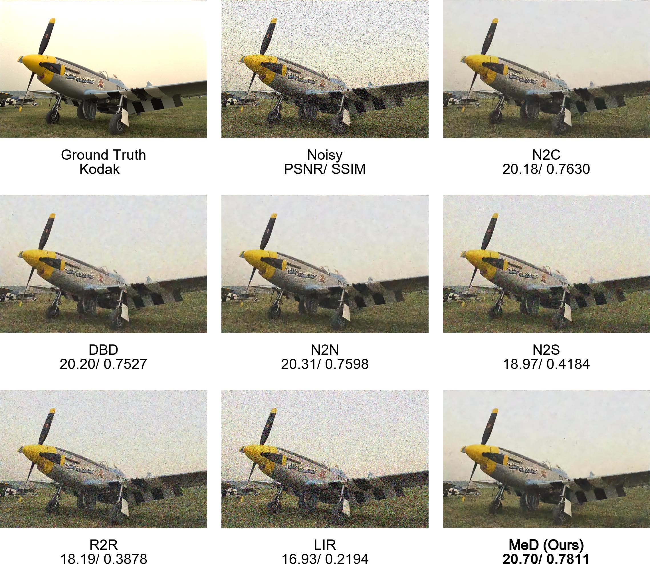
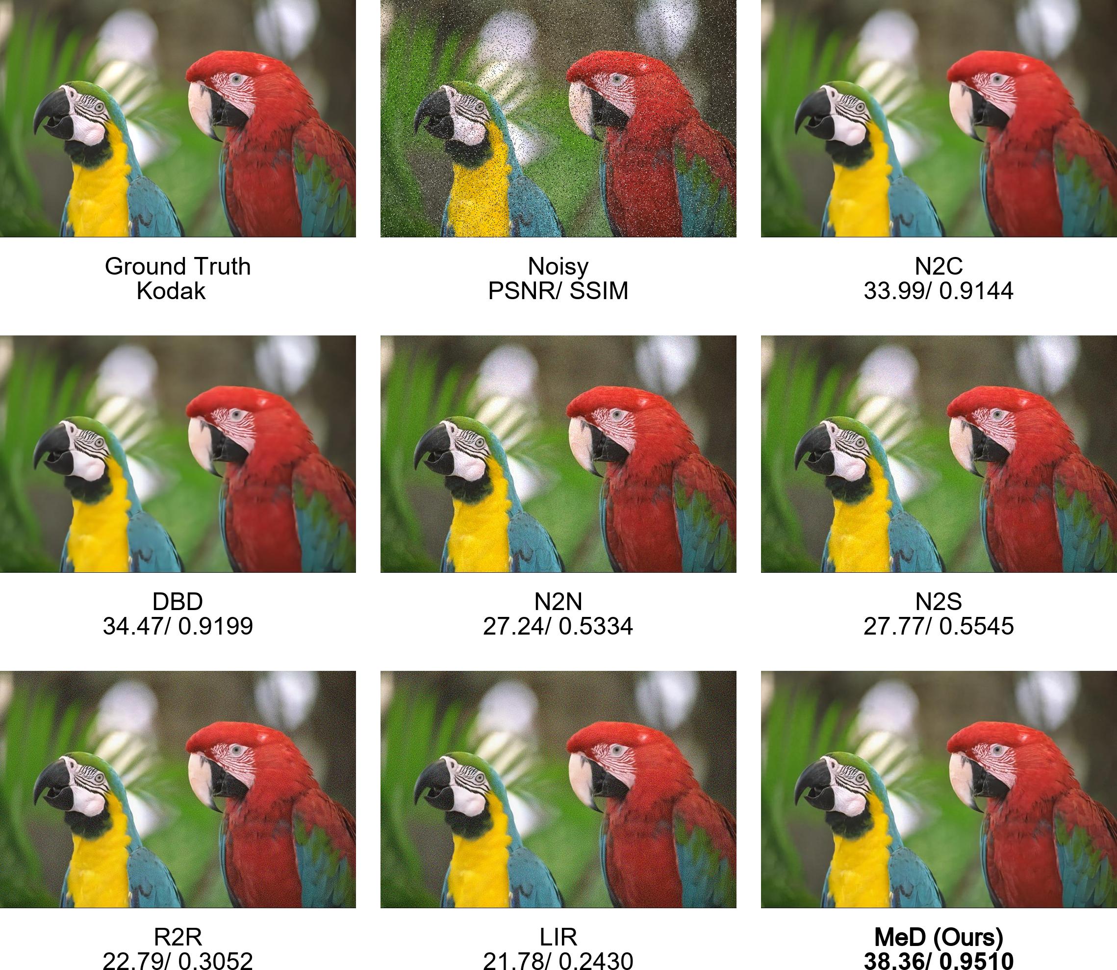
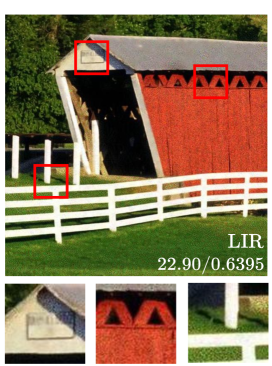
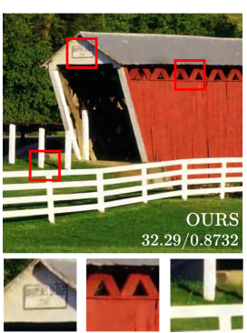
Under this new multi-view setting, we reformulate the task problem as “what is the shared latent information across these views?” instead of the conventional “what is the clean image?” By doing so, MeD can effectively leverage the scene coherence of multi-view data and capture underlying common parts without requiring access to the clean image. This makes it more practical and scalable in real-world scenarios. An example of the proposed method with comparison to prior works is shown in Figure 1, indicating its effectiveness over the state-of-the-art.
Specifically, given any scene image sampled uniformly from a clean image set , MeD produces two contaminated views:
| (1) |
forming two independent corrupted image sets , , where . The and represent two random independent image degradation operations.
We parameterise our scene feature encoder and decoder with and . Considering the image pair , the core of the presented method can be summarised as:
| (2) | |||
| (3) |
where represents the shared scene latent between and with referring to the input image index of . A clean image estimator forms an all-deterministic reverse mapping from to reconstruct an estimated clean image . Similarly, the noise latent is factorised from a corrupted view with a corruption encoder . Afterwords, the resulting corruption is reconstructed from through the use of a corruption decoder, represented by .
The disentanglement is then performed between on a cross compose decoder with parameter , which can be formulated as:
| (4) |
It should be noted that Equation (4) is performed over latent features and from different views. When assuming that remains constant across views, the reconstructed view is determined by the .
Contributions.
The contributions of our work are summarised as follows:
-
•
We propose a new problem formulation to address the ill-posed problem of image denoising using only noisy examples, in a different paradigm than prior works.
-
•
We introduce a disentangled representation learning framework that leverages multiple corrupted views to learn the shared scene latent, by exploiting the coherence across views of the same scene and separating noise and scene in the latent space.
-
•
Extensive experimental analysis validates the effectiveness of the proposed MeD, outperforming existing methods with more robust performance to unknown noise distributions, even better than its supervised counterparts.
2 Related Work
Single-view image restoration:
In [10], Dong et al. were the first to employ a deep network in super-resolution. Later, a range of single view-based models expanded the idea of supervised deep learning to handle image restoration tasks, such as deblurring [17], JPEG artefacts [14], inpainting [20, 38] and denoising [41, 19, 29]. Recently, it is receiving increasing interest in relaxing the prerequisite of supervised learning with corrupted/ clean image pairs. In the context of image denoising, the “corrupted/clean” pair denotes a corrupted input image and its corresponding clean image for calculating the loss. To tackle the issue of the lack of clean data, several methods have been proposed, such as the Noise2Noise (N2N) method [19] and Recorrupted-to-Recorrupted (R2R) [29], which train deep networks on pairs of noisy images. Noise2Void (N2V) [15], Noise2Self (N2S) [5], and the method proposed by Laine et al. [18] are based on the blind-spot strategy that discards some pixels in the input and predicts them using the remaining. In the field of single-image denoising, some methods such as DIP [32] and S2S [30], have achieved remarkable denoising results using only one noisy image.
These methods, however, often inevitably compromise image quality to noise reduction, resulting in over-smoothed output. This trade-off is further exacerbated under domain shifts when dealing with unknown noise distributions.
Restoration based on multiple views:
Existing multi-view variants of image restoration methods mainly focus on sequential data such as video or burst images. For example, Tico [31] builds a paradigm that separates the unique and common features within the multi-frame to produce a denoised estimate. Liu et al. [23] models degrading elements as foreground and estimate background using video data. Deep Burst Denoising (DBD) [13] performs multi-view denoising based on burst images. Each image is taken in a short exposure time and serves as a corrupted observation of the clean image.
Unlike the above-mentioned methods, our MeD aims to use multiple static observations simultaneously to learn the latent representation of a clean scene that is shared by multiple discrete views.
Self-supervised feature disentanglement:
Another notable path of work has attempted to disentangle underlying invariant content from distorted images. For instance, UID-GAN [25] utilises unpaired clean/blurred images to disentangle content and blurring effects in the feature space and yield improved deblurring performance. Similarly, LIR [11] used unpaired input to isolate invariant content features through self-supervised inter-domain transformation.
However, these methods are limited to synthetic noise and do not extend well in real-world scenarios due to their reliance on clean images. In contrast, our method is purely based on multiple noisy views of the same static scene and aims to disentangle the scene from corruption, without the need for clean image supervision.
3 Methodology
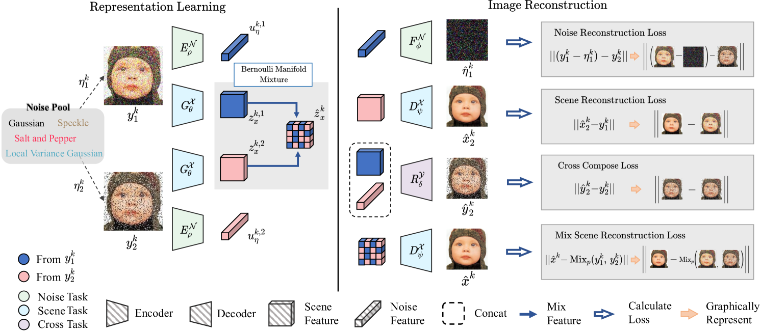
Our primary objective is to identify the commonalities among different views in the denoising process. To achieve this, we aim to discover the shared scene that is degradation-agnostic over various corrupted views via our proposed training schema, namely Multi-view self-supervised Disentanglement (MeD). A graphic depiction of MeD is shown in Figure 2, composed of the representation learning process in the left panel, and four distinct reconstruction pathways in the right panel.
The detailed design of the proposed schema will be introduced in the following subsections. Section 3.1 explains the restoration of noise and scene. Section 3.2 details the reconstruction of noisy input using a cross-feature combination. Section 3.3 elaborates on the reconstruction of the scene using mixed scene latent.
We will start our introduction by outlining three essential properties that a multi-view representation disentanglement technique should exhibit.
Pre-assumed properties:
Suppose the scene latent space and corruption latent space are symbolised by and , respectively.
-
(1)
Independence: For any scene latent , it is expected to be independent of any corruption latent .
-
(2)
Consistency: There exists one shared latent code that is capable of representing the shared clean component of all instances in the set .
-
(3)
Composability: Recovery of the corrupted view can be achieved using the feature pairs , and the index of the recovered view is determined by the index of the corruption latent, which represents the unique component within that particular view.
A key step of our method is to realise these pre-requisitions by determining how to implement the latent space assumption. As shown in the left panel of Figure 2, to infer our latent space assumption, MeD is comprised of two encoders and three decoders: A shared content latent encoder and its decoder , an auxiliary noise latent encoder and its decoder , and a cross disentanglement decoder .
3.1 Main Forward Process
Given two corrupted views of the same image , and , the encoder mainly perform the scene feature space encoding that can be formulated as:
| (5) |
where and are the estimation of the scene feature corresponding to the inputs and .
The process of clean image reconstruction is then completed by the :
| (6) |
Similar to the process of estimating scene features, the estimation of distortion features by , followed by the reconstruction of noise with , can be described as follows:
| (7) |
We adhere to the methodology introduced by N2N [19] to use noisy images as supervisory signals. The objective function of the aforementioned process can be simplified to:
| (8) |
The objective of and are the same as above, with only a subscript difference. It should be noted that, although our objective functions are similar to that of N2N, our goal is not simply to find and remove noise, but rather to capture the common features shared across multiple views.
3.2 Cross Disentanglement
For general latent codes to sufficiently represent scene information in the image space, it is natural to assume that these codes exhibit a certain degree of freedom, allowing them to intersect with the noise space. Consequently, there is no guarantee of complete isolation between and . To meet the requirements of properties (1) and (3), we use an additional decoder to reconstruct a corrupted view over a cross-feature combination, e.g. from and from , which can be represented as:
| (9) |
This realisation explicitly requires to represent the common part and to represent the unique part within the corrupted views. We then optimise from using the following objective:
| (10) |
3.3 Bernoulli Manifold Mixture
The aforementioned latent constraint might appear to be restricted at first, but in fact, it enables us to capture a large number of degrees of freedom in latent space implementation. For instance, it is possible to have multiple scene features that correspond to a single scene. However, in such cases, the mapping from input to scene features becomes ambiguous. To tackle this issue, we propose the use of the Bernoulli Manifold Mixture (BMM) as a means of leveraging the shared structure within the scene latent.
Given the assumption of property (2), the acquired scene features and are expected to be identical and interchangeable with one another, as they both refer to the same scene feature. BMM establishes a new explicit connection between the scene features of multi-views, which can be expressed in the equation as:
| (11) |
where the is an estimation of the true underlying scene feature. Let define a sample instance drawn from a Bernoulli distribution with probability , the function described in Equation (11) denotes:
| (12) |
By establishing this new connection (Equation 11), we can enhance the interchangeability between and by optimising the reconstruction performance on .
Lemma 1. Assuming , where denotes multivariate Gaussian distributions and then and is the mean and the covariance matrix.
For a given function , assume , the following property holds:
| (13) |
Proof. Assume are i.i.d., we may also factorise . Write
| (14) |
so that we can have
| (15) |
with the fact that Bernoulli sample = , the mixed feature is in the same representation distribution as .
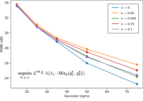
In MeD, we denote = , and the objective for implementing Equation (13) can be formulated as follows:
| (16) |
where the is the weight parameter. Here, the target is using a mixed version of and . The choice of this is driven by the intuition that the hybrid version would better align with the aforementioned blended features.
4 Experiments
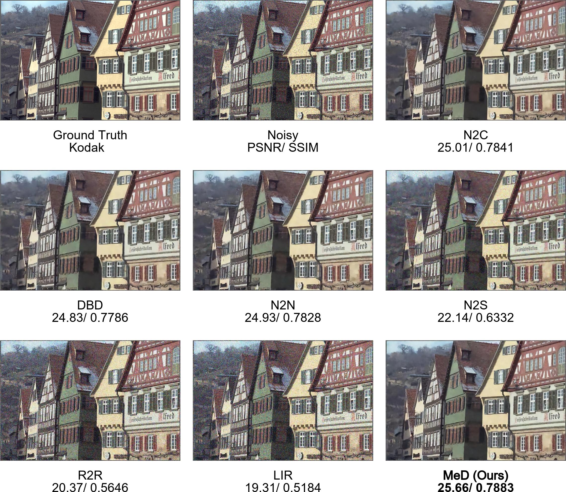
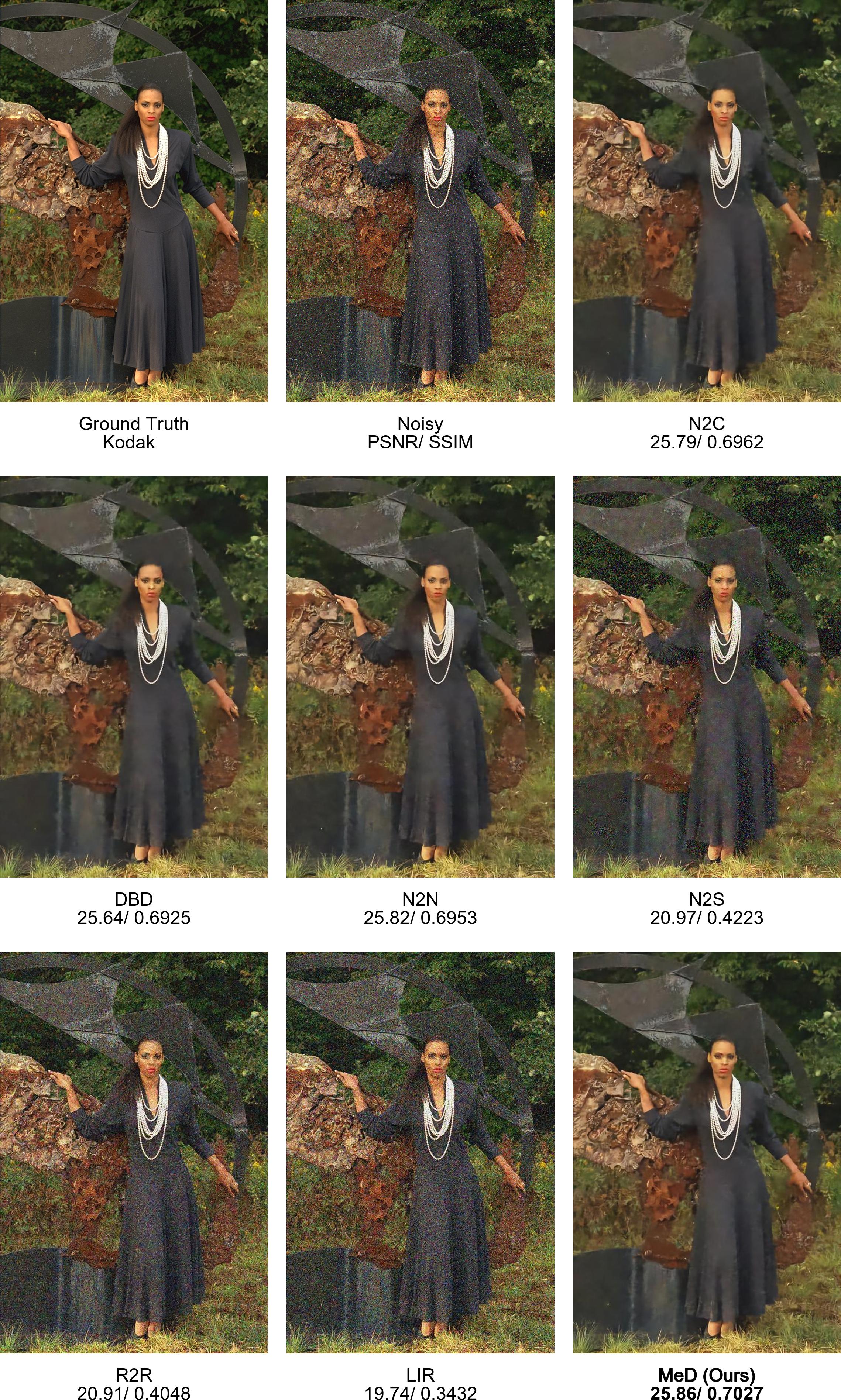
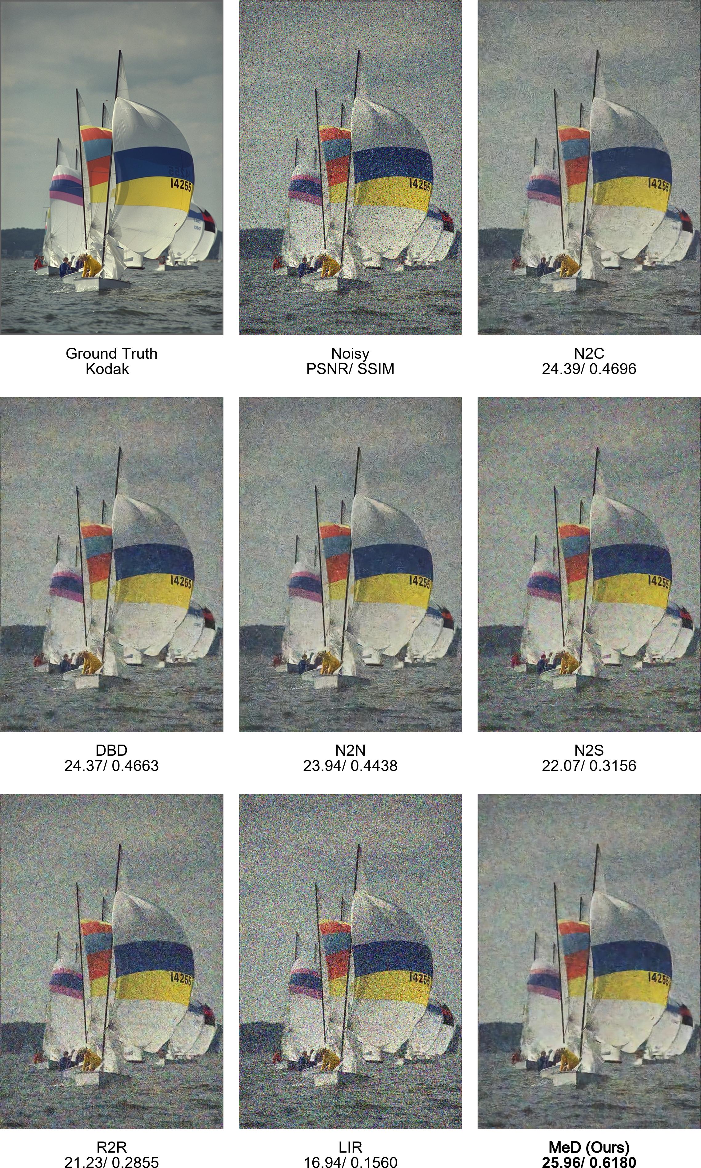
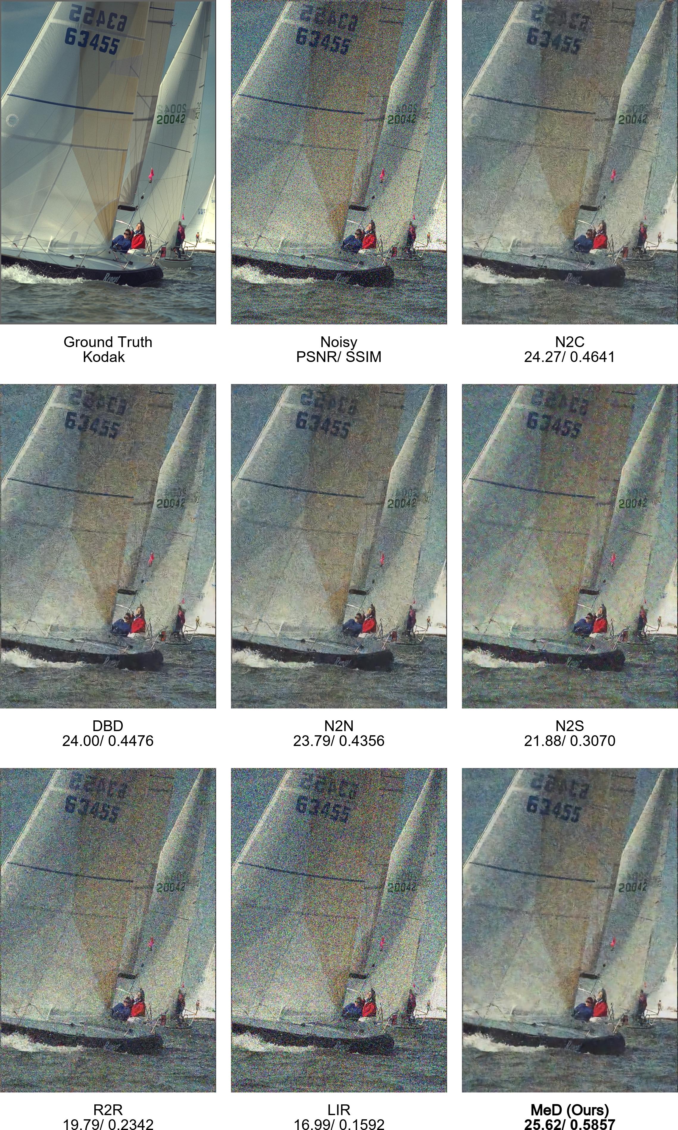
To evaluate the effectiveness of our proposed method, we assess our method against several representative self-supervised denoising methods, including Noise2Noise (N2N) [19], Noise2Self (N2S) [5] and Recorrupted2Recorrupted (R2R) [29], and the invariant feature learning method LIR [11]. Moreover, we also evaluate our approach against two supervised baseline methods (Noise2Clean (N2C) [24] and multi-frame method DBD [13]) to further validate its effectiveness. Comparisons to more methods, including methods using only one noisy image, are presented in the supplementary Table 10.
We start our experiments by denoising synthetic additive white Gaussian noise (AWGN) in Section 4.2, and then move on to testing unseen noise levels and noise types in Section 4.3 and Section 4.4, respectively. Furthermore, we evaluate the performance in real-world scenarios in Section 4.5. In Section 4.6, we expand our experiments to incorporate more views to study their impact on performance. Finally, in Section 4.7, we apply our method to other tasks, e.g. image super-resolution and inpainting, to demonstrate its generalisation ability.
4.1 Experimental Setups
Noted that, the nature of feature disentanglement requires no leak from input to output, however, the global residual connection of the original DnCNN [41] cannot satisfy. Thus, we incorporate the Swin-Transformer (Swin-T) [24] instead of the traditionally used DnCNN in our experiments. Nevertheless, as Swin-T is not originally designed for image restoration, we make some modifications to enforce local dependence across the image. Specifically, we add one Convolution Layer each before the patch embedding and after the patch unembedding of Swin-T, as inspired by SwinIR [21]. The resulting modified network backbone is denoted as Swin-Tx.
To ensure a fair comparison, we use the Swin-Tx backbone for all methods in our study, except for DBD. As DBD did not release the code, we follow the instructions presented in the paper and make our best effort to re-implement it. However, we observe that the two-view DBD could not converge efficiently, which is consistent with the findings in the paper. Therefore, we limit our evaluation to the four-view DBD, denoted as DBD4. Furthermore, we replace the U-Net backbone originally used in the LIR method with Swin-Tx to maintain consistency in our evaluation. This results in an average improvement of approximately 1 dB in PSNR for Gaussian denoising.
In all experiments, all methods were trained using only DIV2K [4] and the same optimisation parameters, except for LIR and which used manually selected parameters obtained through experiments. For more training and evaluation details including the choice of parameters, please refer to the supplementary Section B. Code is available at: https://github.com/chqwer2/Multi-view-Self-supervised-Disentanglement-Denoising.
Remark:
In tables, the best results are highlighted in bold, while the second best is underlined.
| Training | Test | Noisy/ Clean | Noisy/ Noisy | Invariant Feature | ||||
| Schema | N2C [24] | DBD4 [13] | N2N [19] | N2S [5] | R2R [29] | LIR [11] | MeD (ours) | |
| Gaussian | 15 | 33.36/ 0.9020 | 33.57/ 0.9092 | 32.64/ 0.8805 | 32.77/ 0.8780 | 29.74/0.7865 | 31.06/ 0.8632 | 33.11/ 0.8880 |
| 25 | 30.83/ 0.8494 | 31.31/ 0.8548 | 30.68/ 0.8334 | 30.99/ 0.8405 | 30.45/0.8183 | 30.01/ 0.8024 | 30.57/ 0.8496 | |
| 50 | 24.76/ 0.5519 | 25.12/ 0.5583 | 24.59/ 0.5385 | 22.13/ 0.3928 | 24.02/0.5133 | 21.97/ 0.3578 | 25.67/ 0.6026 | |
| 75 | 20.75/ 0.3376 | 21.09/ 0.3412 | 20.60/ 0.3162 | 17.86/ 0.1998 | 19.10/0.2641 | 16.23/ 0.1689 | 23.09/ 0.4320 | |
| Gaussian | 15 | 33.47/ 0.9027 | 33.12/ 0.8915 | 33.45/ 0.8945 | 31.28/ 0.8187 | 20.76/ 0.2508 | 30.85/ 0.8431 | 33.62/ 0.9026 |
| 25 | 30.87/ 0.8538 | 30.64/ 0.8491 | 30.77/ 0.8423 | 29.65/ 0.7801 | 23.91/ 0.4552 | 28.92/ 0.8069 | 30.91/ 0.8573 | |
| 50 | 27.41/ 0.7361 | 27.13/ 0.7290 | 27.15/ 0.7219 | 27.00/ 0.7114 | 26.92/ 0.6911 | 25.13/ 0.6191 | 27.48/ 0.7530 | |
| 75 | 25.05/ 0.6223 | 24.97/ 0.6205 | 24.80/ 0.5908 | 24.89/ 0.6023 | 23.83/ 0.5132 | 22.37/ 0.4212 | 25.40/ 0.6645 | |
| Fine-tuning Method | N2C [24] | N2N [19] | LIR [11] | MeD | |||
| Pretraining Method | N2C | MeD | N2N | MeD | LIR | MeD | MeD |
| Gaussian, | 29.20/ 0.7797 | 29.53/ 0.8081 | 29.04/ 0.7642 | 29.21/ 0.7890 | 26.42/ 0.6640 | 27.25/ 0.7036 | 29.60/ 0.8101 |
| Local Var Gaussian | 35.62/ 0.9308 | 35.85/ 0.9439 | 35.66/ 0.9256 | 35.73/ 0.9310 | 29.26/ 0.8170 | 30.51/ 0.8387 | 35.91/ 0.9762 |
| Poisson Noise | 40.49/ 0.9736 | 42.80/ 0.9776 | 41.35/ 0.9736 | 42.27/ 0.9813 | 31.23/ 0.8672 | 33.47/ 0.8932 | 45.05/ 0.9826 |
| Speckle, | 33.36/ 0.9004 | 33.40/ 0.9044 | 33.32/ 0.8931 | 33.33/ 0.8907 | 28.28/ 0.7713 | 29.82/ 0.8229 | 33.48/ 0.9115 |
| S&P, | 28.85/ 0.8267 | 30.73/ 0.8372 | 28.59/ 0.8003 | 29.45/ 0.8255 | 26.69/ 0.7241 | 27.62/ 0.7460 | 30.84/ 0.9135 |
| Average | 33.50/ 0.8822 | 34.46/ 0.8942 | 33.59/ 0.8714 | 34.00/ 0.8835 | 28.38/ 0.7687 | 29.73/ 0.8009 | 34.98/ 0.9188 |
4.2 AWGN Noise Removal
We first investigate the denoising generalisation of the methods using synthetic zero-mean additive white Gaussian noise (AWGN). The experiments are divided into two parts. The first segment employs fixed variance AWGN, whereas the second segment employs varied variance Gaussian for training in a separate manner. Table 1 summarises the quantitative results evaluated on CBSD68 Dataset [26] at variance levels of 15, 25, 50, and 75.
Analysis: In the fixed variance setting, MeD performs inferior compared to the other methods on lower noise levels of 15 and 25. However, as the methods face more severe corruption, MeD outperforms all self-supervised and supervised methods, showing our greater advantage of handling severe noise. For instance, at , MeD outperforms the second-best method (N2C) by around 2 dB. These results suggest that MeD has a remarkable ability to generalise to a range of unseen noise levels in Gaussian noise.
In the context of random variance, it has been observed that MeD exhibits superior performance across all four noise levels compared to other methods, including supervised methods. These findings imply that MeD can benefit more from varying training noise than other methods. More experiments and details on AWGN noise removal can be found in the supplementary Table 9.
 |
 |
 |
 |
 |
 |
 |
 |
 |
| McM-17 [42] | Reference | N2C [41] | DBD [13] | N2N [19] | N2S [5] | R2R [29] | LIR [11] | MeD (Ours) |
| Speckle | PSNR/SSIM | 27.58/ 0.7712 | 28.10/ 0.7347 | 27.06/ 0.7452 | 26.99/ 0.7338 | 25.56/ 0.5529 | 23.29/ 0.5681 | 28.57/ 0.7722 |
|
 |
 |
 |
 |
 |
 |
 |
 |
| McM-01 [42] | Reference | N2C [41] | DBD [13] | N2N [19] | N2S [5] | R2R [29] | LIR [11] | MeD (Ours) |
| Gaussian | PSNR/SSIM | 27.09/ 0.6561 | 26.77/ 0.4824 | 26.84/ 0.5177 | 26.64/ 0.4359 | 25.5/ 0.5451 | 23.24/ 0.2298 | 27.91/ 0.7651 |
 |
 |
 |
 |
 |
 |
 |
 |
 |
| Kodak-21 [12] | Reference | N2C [41] | DBD [13] | N2N [19] | N2S [5] | R2R [29] | LIR [11] | MeD (Ours) |
| S&P | PSNR/SSIM | 33.26/ 0.9224 | 34.25/ 0.9413 | 30.83/ 0.8857 | 31.07/ 0.8864 | 29.03/ 0.8377 | 27.40/ 0.6498 | 36.83/ 0.9246 |
4.3 Generalisation on Unseen Noise Removal
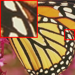
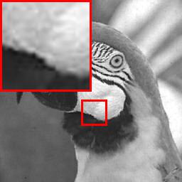
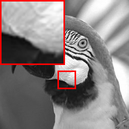
In the previous subsection, we demonstrated the remarkable generalisation ability of our model in the case of Gaussian noise. Here, we aim to extend this investigation to other types of unseen noise and evaluate the denoising generalisation ability of our method. Specifically, we consider Poisson noise, Speckle noise, Local Variance Gaussian noise, and Salt-and-Pepper noise. For a more detailed synthetic process, please refer to the supplementary Section F.
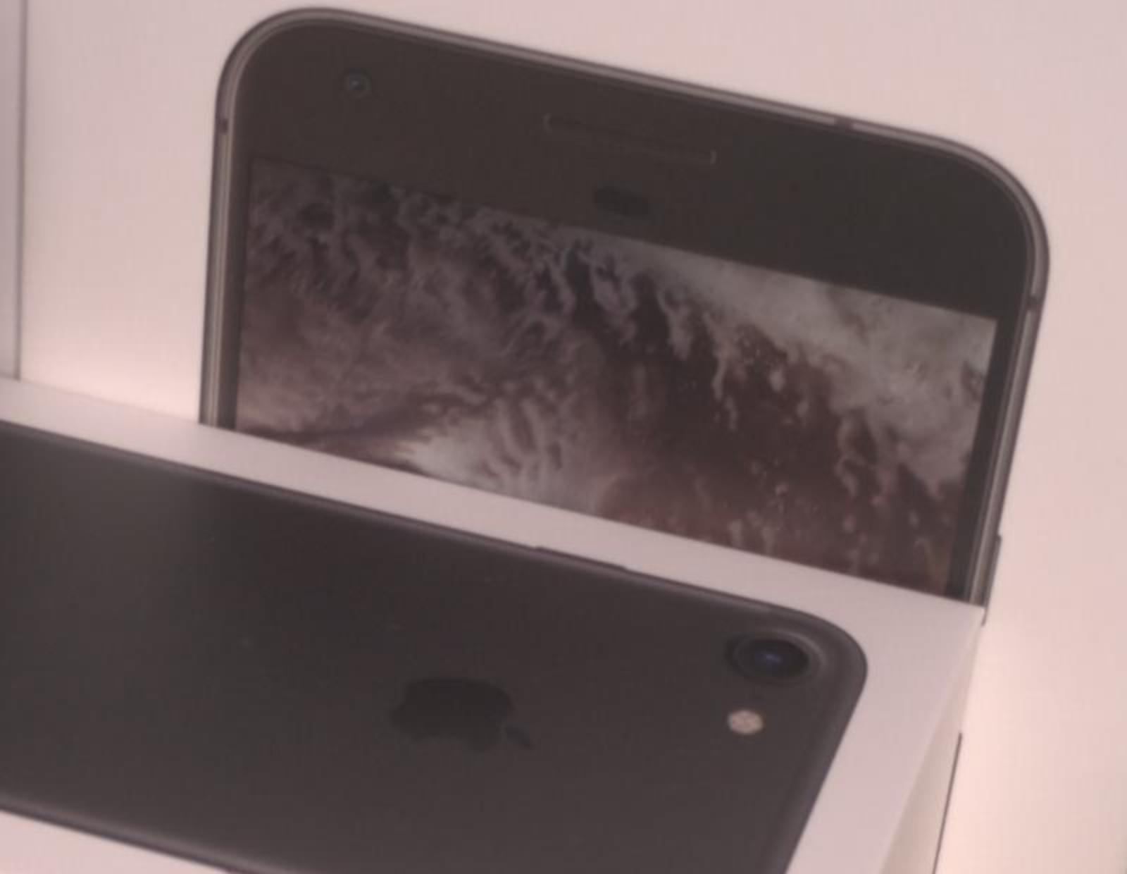
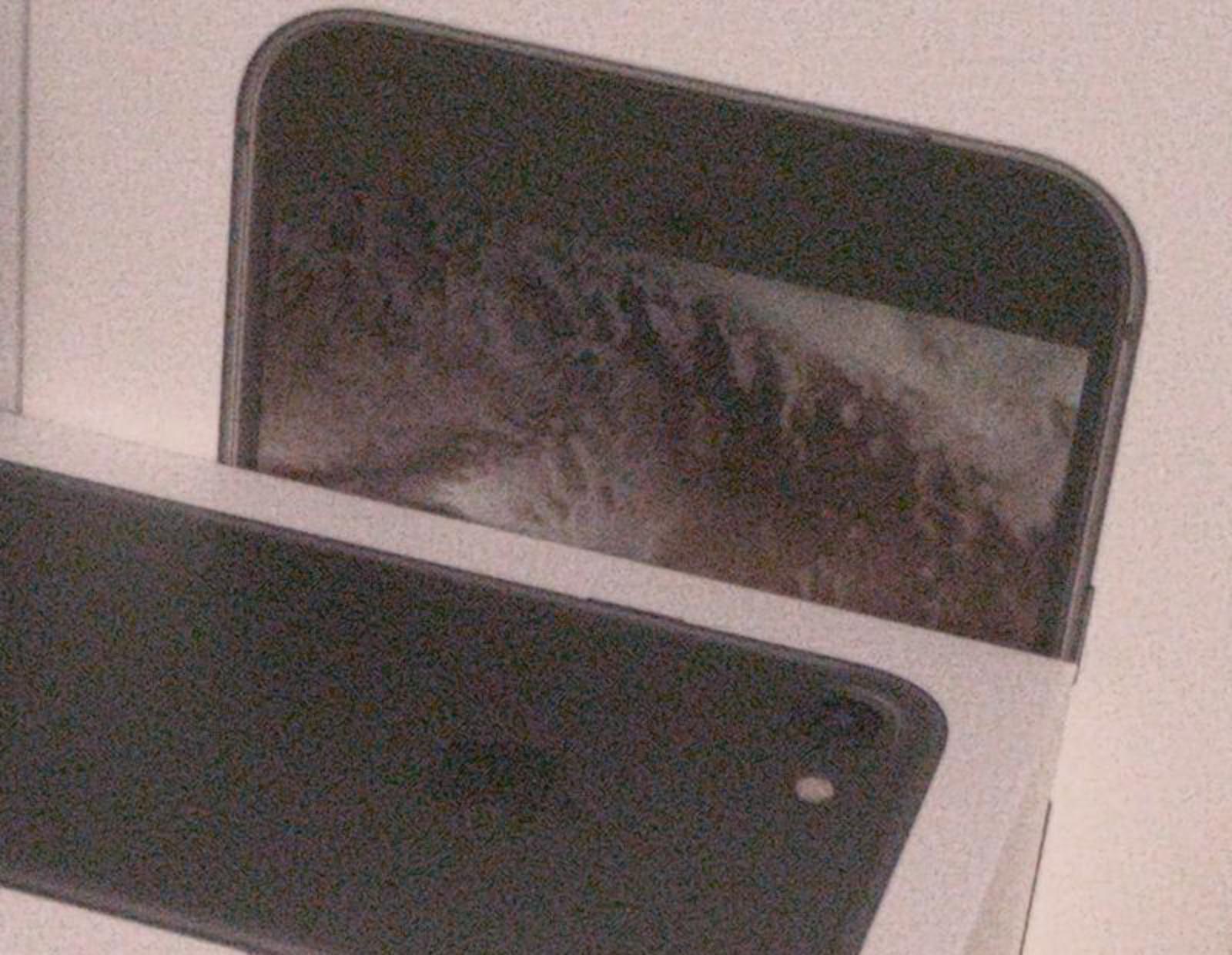
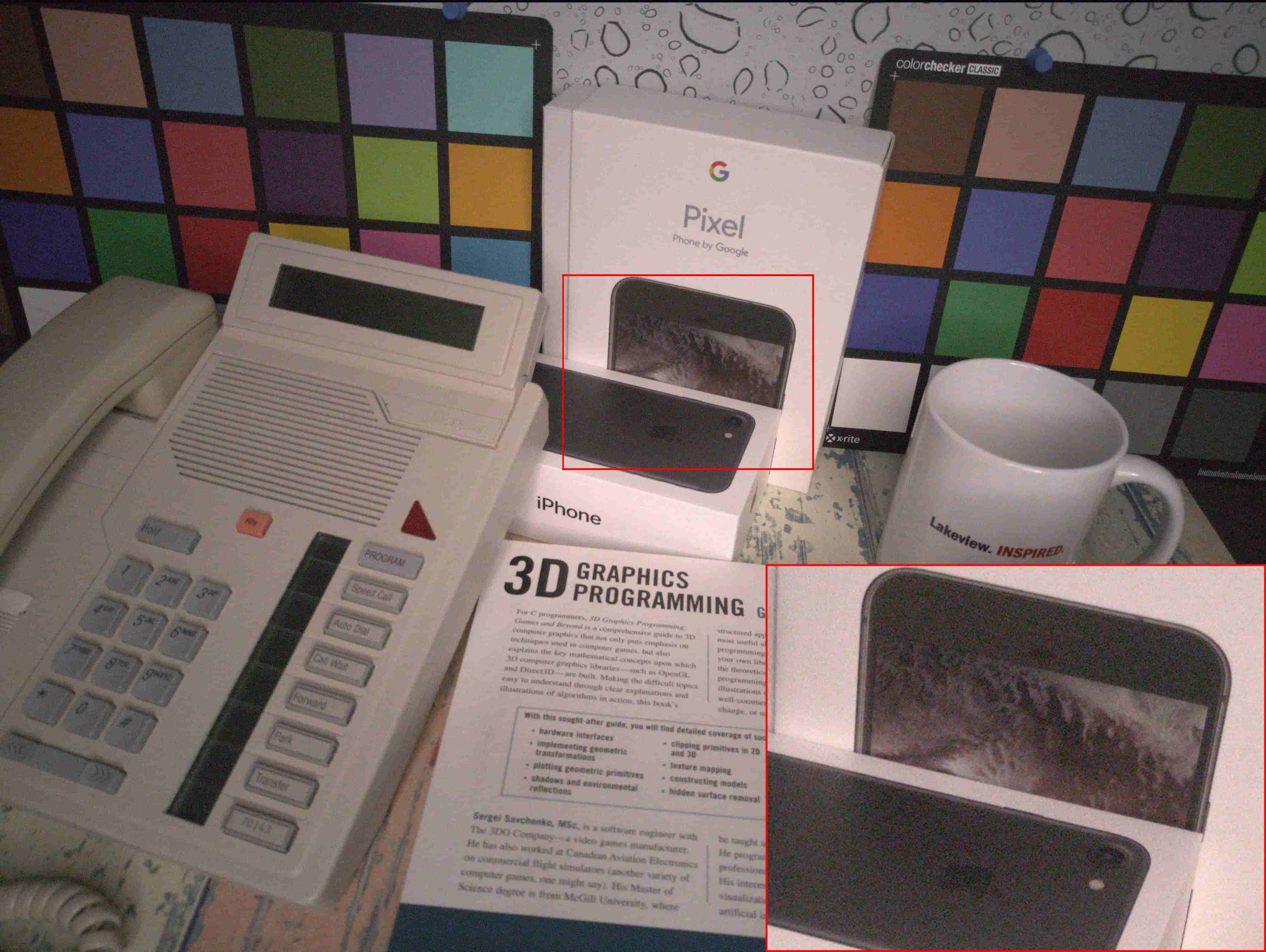
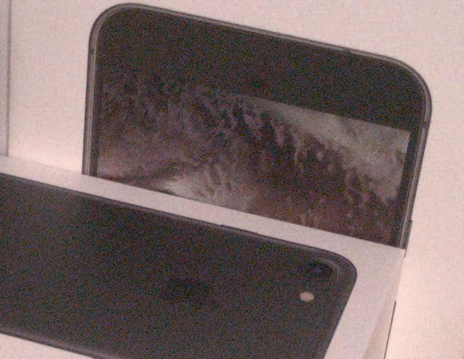
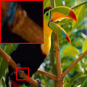
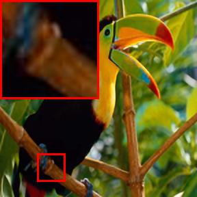
First, we demonstrate qualitative comparisons of denoising unseen noise types using models trained only with Gaussian in Figure 3. Next, in order to further verify the denoising generalisation ability of MeD, we employ its scene encoder and decoder as pre-trained models to be compared against other methods. It should be noted that the pre-training and fine-tuning methods employed in this study may differ, as shown in Table 2. The pre-training of all test models was conducted on a Gaussian sigma value of 25, followed by fine-tuning with a Gaussian sigma range of 5 to 50. Since the training schema of N2S, R2R, and DBD4 differs from MeD, we do not include them in this section. However, evaluations of these methods on unseen noise are still presented in Section 4.4 under different settings.
| Test Noise | Noisy/ Clean | Noisy/ Noisy | Invariant Feature | ||||
| N2C [24] | DBD4 [13] | N2N [19] | N2S [5] | R2R [29] | LIR [11] | MeD (ours) | |
| Gaussian, | 29.24/ 0.7754 | 29.05/ 0.7616 | 29.23/ 0.7634 | 28.58/ 0.7589 | 26.43/ 0.6639 | 26.67/ 0.6866 | 29.61/ 0.8178 |
| Local Var Gaussian (LVG) | 36.64/ 0.9442 | 36.18/ 0.9307 | 36.65/ 0.9235 | 33.24/ 0.8858 | 34.70/ 0.8779 | 31.61/ 0.8627 | 37.99/ 0.9568 |
| Poisson Noise | 45.72/ 0.9764 | 44.23/ 0.9606 | 45.64/ 0.9799 | 46.31/ 0.9808 | 44.45/ 0.9491 | 43.27/ 0.9292 | 48.10/ 0.9916 |
| Speckle, | 35.58/ 0.9417 | 35.24/ 0.9385 | 35.34/ 0.9475 | 35.13/ 0.9596 | 34.20/ 0.9078 | 33.98/ 0.8810 | 37.21/ 0.9715 |
| S&P, | 38.85/ 0.9165 | 37.10/ 0.8884 | 38.89/ 0.9289 | 38.22/ 0.9330 | 36.17/ 0.9087 | 33.43/ 0.8202 | 42.33/ 0.9695 |
| Gaussian + Speckle | 30.19/ 0.8279 | 29.24/ 0.8156 | 30.32/ 0.8317 | 29.51/ 0.8050 | 28.78/ 0.7744 | 29.20/ 0.7871 | 31.92/ 0.8726 |
| Gaussian + Speckle | 27.30/ 0.7251 | 26.55/ 0.7126 | 27.23/ 0.7331 | 26.91/ 0.7081 | 26.49/ 0.6935 | 26.19/ 0.6941 | 29.68/ 0.7928 |
| LVG + Poisson | 31.78/ 0.9087 | 31.10/ 0.8842 | 31.60/ 0.7617 | 30.15/ 0.8086 | 28.52/ 0.7144 | 27.33/ 0.7234 | 34.29/ 0.9325 |
| Poisson + Speckle | 31.39/ 0.9069 | 30.86/ 0.8782 | 31.52/ 0.8935 | 30.58/ 0.9067 | 30.34/ 0.8897 | 29.93/ 0.8554 | 33.04/ 0.9258 |
| Average | 34.08/ 0.8803 | 33.28/ 0.8634 | 34.05/ 0.8626 | 33.18/ 0.8607 | 32.23/ 0.8199 | 31.29/ 0.8044 | 36.02/ 0.9145 |
Analysis: Qualitative results in Figure 3 show that under Gaussian training settings, our method surpasses other methods in denoising unseen noise types. Additionally, Table 2 shows that the approaches using pre-trained MeD models outperform their self-transfer models for N2C, N2N, and LIR, with improvements of up to 2 dB in some cases. On average, the MeD pre-trained models show a performance gain of around 0.5 dB across all methods, highlighting the potential of MeD as a powerful pre-training method for image denoising. It is noteworthy that the self-transfer MeD model exhibits the best denoising performance across all validation noise types, even outperforming the supervised method, N2C. This is particularly evident in Poisson noise, where MeD surpasses N2C by 3 dB. These results highlight the generalisation ability of our approach in handling unseen noise.
4.4 Experiments on General Noise Pool
Here we further investigate the generalisation ability of our method by introducing our general Noise Pool. The Noise Pool comprises the five aforementioned types of noise, each with a diverse range of noise levels. During training, we randomly sample from the noise pool to provide the model with noisy images. This novel approach simulates a realistic scenario where noise is unknown and can originate from various sources to some extent.
Specifically, we evaluated all methods using the random noise pool approach to train and test on combined or single noise types. The results are summarised in Table 3.
 |
 |
 |
 |
|
| PSNR/ SSIM | 31.38/ 0.8912 | 30.19/ 0.7449 | 29.60/ 0.7053 | |
| Ground Truth [1] | N2C [24] | DBD4 [13] | N2N [19] | |
 |
 |
 |
 |
 |
| 23.68/ 0.2967 | 28.58/ 0.6081 | 26.58/ 0.4257 | 25.91/ 0.3795 | 33.07/ 0.8849 |
| Noisy Image from SIDD [1] (ISO 800) | N2S [5] | R2R [29] | LIR [11] | MeD (Ours) |
 |
 |
 |
 |
|
| PSNR/ SSIM | 28.36/ 0.5661 | 27.58/ 0.5406 | 27.23/ 0.49 | |
| Reference | N2C [24] | DBD4 [13] | N2N [19] | |
 |
 |
 |
 |
 |
| 25.33/ 0.3865 | 27.58/ 0.5516 | 26.77/ 0.4889 | 26.45/ 0.4752 | 30.23/ 0.6703 |
| Noisy Image from SIDD | N2S [5] | R2R [29] | LIR [11] | MeD (Ours) |
Analysis: In Table 3, our MeD approach outperforms all other methods significantly on all the test noise types. For example, when a test noise containing a combination of Gaussian noise with and Speckle noise with is used, other methods exhibit an approximate performance of 27 dB. However, MeD achieves significantly better results with a performance of 29.68 dB. And on average, MeD exhibits a performance that is approximately 2 dB better than other methods. Our findings show that utilising a comprehensive noise pool for training purposes can effectively improve the generalisation capability. Furthermore, the remarkable denoising generalisation ability of our MeD approach, in comparison to other methods, is particularly advantageous for real-world applications.
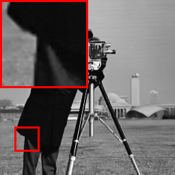
4.5 Real Noise Removal
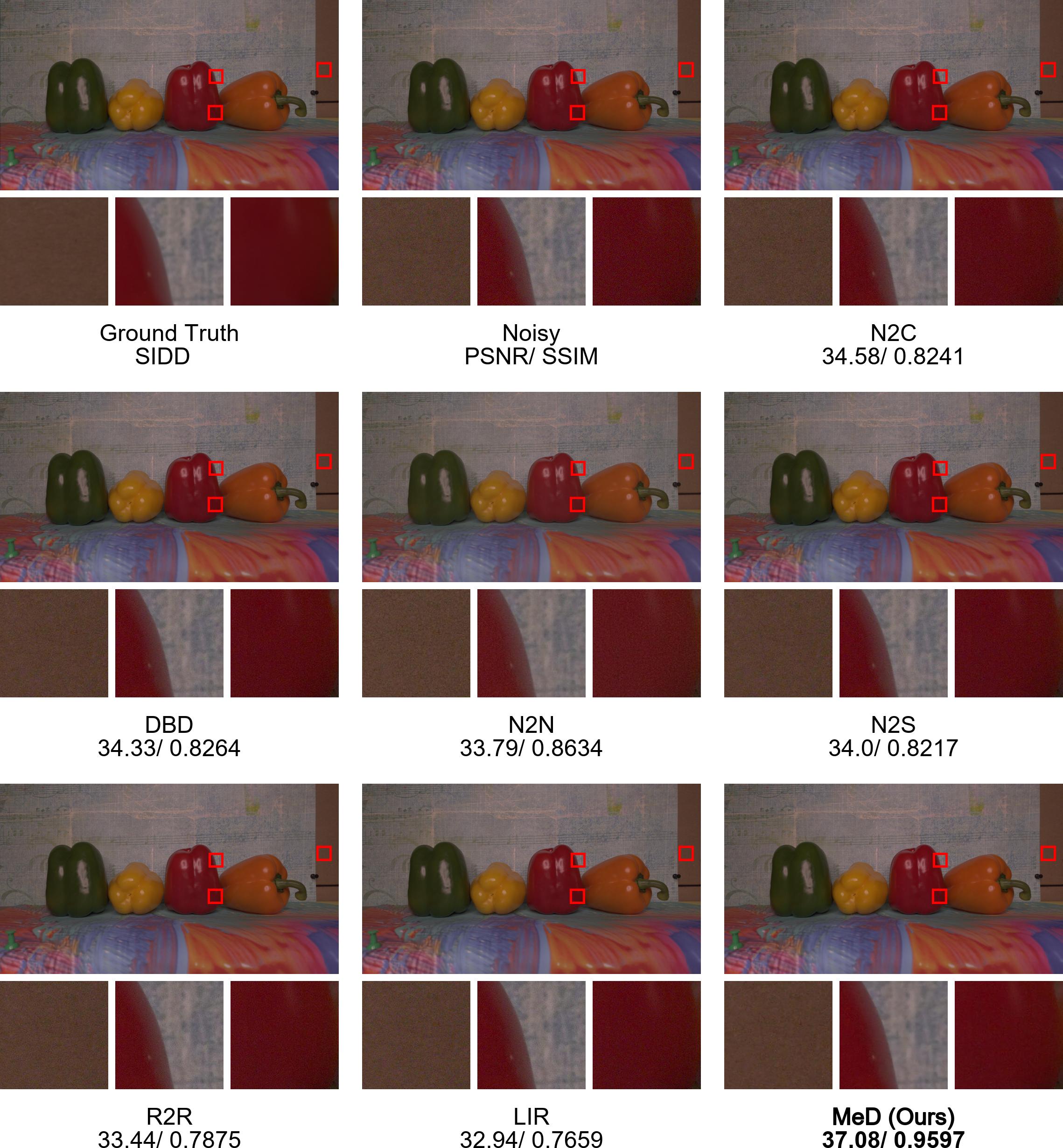
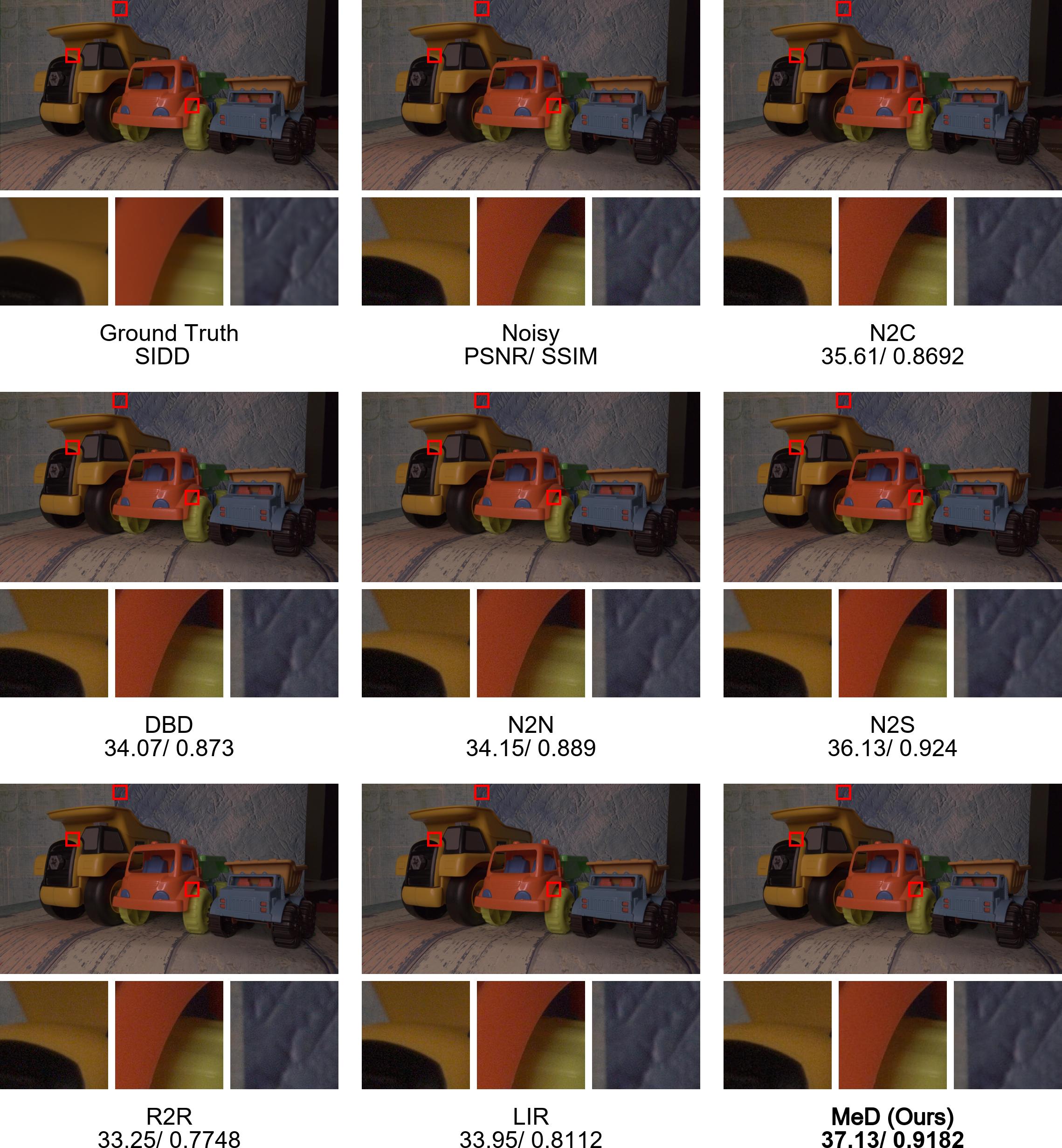
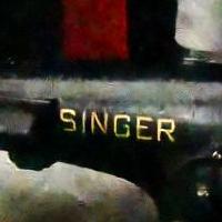
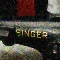
In our previous experiments, we demonstrated the exceptional denoising performance of our MeD approach on synthetic noises. However, real-world noise is often more complex and challenging than synthetic noise. In this subsection, we aim to evaluate the generalisation performance of our approach on real-world noise by testing it on the SIDD [1], CC [27] and PolyU [36] datasets. To assess the denoising performance on real-world noise, we use the same pre-trained models as in Section 4.4. The representative qualitative results on the SIDD dataset in the standard RGB colour space are presented in Figure 4.
| Method | PolyU [36] | SIDD [1] | CC [27] | Average |
| N2C [24] | 35.89/ 0.9652 | 30.37/ 0.6028 | 37.89/ 0.9408 | 34.72/ 0.8363 |
| DBD4 [13] | 35.69/ 0.9571 | 30.23/ 0.6173 | 37.74/ 0.9357 | 34.55/ 0.8367 |
| N2N [19] | 36.22/ 0.9679 | 32.82/ 0.7297 | 37.39/ 0.9570 | 35.48/ 0.8849 |
| N2S [5] | 36.41/ 0.9721 | 30.98/ 0.6018 | 37.58/ 0.9622 | 34.99/ 0.8454 |
| R2R [29] | 34.58/ 0.8890 | 29.64/ 0.5708 | 35.35/ 0.8478 | 33.19/ 0.7692 |
| LIR [11] | 34.81/ 0.7278 | 28.76/ 0.5296 | 35.50/ 0.8403 | 33.02/ 0.6992 |
| MeD (ours) | 38.65/ 0.9855 | 35.81/ 0.8278 | 40.08/ 0.9745 | 38.18/ 0.9293 |
Analysis: As shown in Table 4, our approach significantly outperforms all other methods across all three datasets, with a performance improvement of 2-3 dB over the second-best approach, and also consistently outperforms its supervised counterparts (i.e. N2C and DBD4) by over 3 dB. These results suggest the effectiveness and generalisability of the proposed approach in real-world denoising scenarios.
Our approach achieves remarkable performance on real-world noise without even being trained on more expensive real-world data. For a more complete study, we also conduct experiments on model training with real-world data (more details please refer to the supplementary Table 11), showing superior performance and even better generalisation ability to data out of the training data distribution.
In Figure 4, the presence of noise persists even after applying denoising techniques, yet ours demonstrates the most authentic outcomes compared to others. For instance, while the noise particles remain prominent in the N2C results, they are absent in our results. Overall, the results indicate that the MeD approach is well-suited for real-world denoising tasks, providing a robust and reliable solution for improving image quality in challenging environments.
4.6 Expand to More Views
Although we only showcase two views for the experiments above, our method can be easily expanded to multiple views. To investigate the impact of the numbers of views, here we further conduct a study comparing 2, 3, and 4 views, in Table 5.
| #Views | Gaussian | LVG | Poission | Speckle | S&P |
| 2 | 29.61/ 0.8178 | 37.99/ 0.9568 | 48.10/ 0.9916 | 37.21/ 0.9715 | 42.33/ 0.9695 |
| 3 | 29.68/ 0.8197 | 38.05/ 0.9577 | 48.23/ 0.9920 | 37.40/ 0.9733 | 42.45/ 0.9703 |
| 4 | 29.70/ 0.8204 | 38.08/ 0.9580 | 48.31/ 0.9921 | 37.47/ 0.9740 | 42.49/ 0.9709 |
The results indicate that increasing the number of views consistently improves the performance across different noise types. For example, when dealing with Speckle noise, the 4-view model achieves a 0.26 dB higher PSNR than the 2-view model. However, it is worth noting that employing views requires cross-computations within each view pair during training, resulting in a significant increase in computational cost (e.g. from 2-view to 4-view leads to a training time increase in our experiment).
4.7 More Application Exploration
Here we investigate the potential of the proposed MeD for other more general image restoration tasks, such as image super-resolution and inpainting. In this study, we generalise the previously defined degradation (noise) to a residual image between a clean image and a corrupted image. Moreover, we expand the definition from Noise Pool to a more general one – Corruption Pool that contains not only noise but also general corruption.
Super resolution.
Image super-resolution aims to enlarge the resolution of a low-resolution image. We train our method on the DIV2K dataset [4], where we randomly choose different downscale methods from a Corruption Pool that consists of random Gaussian noise and four types of down-scaling (bicubic, lanczos, bilinear, and hamming). We benchmark our method against the supervised method RCAN [44] that aims for high PSNR and the recent unsupervised methods DASR [33] that are specialised for super-resolution. We conduct our evaluation on the Set5 dataset [7] with scaling factors of 2, 3, and 4. The results in Table 6 show the effectiveness of our method over both supervised and unsupervised approaches.
Inpainting.
We also apply our method to the image inpainting task, which fills in missing pixels. We choose two single-image deep learning methods – Self2Self (S2S) [30] and DIP [32], for comparison. Our MeD is trained with Corruption Pool containing noises, down-scaling, and inpainting mask operations altogether. To compare our method (MeD) with other state-of-the-art methods, we conduct experiments on the Set 11 dataset [32] with three different pixel dropping ratios: 50%, 70%, and 90%. The results are shown in Table 7, suggesting the effectiveness of MeD again in the image inpainting task.
5 Conclusion
In this paper, we have presented a new self-supervised learning method (MeD) for image denoising that disentangles scene and noise features in a constraint feature space. Our approach has demonstrated exceptional denoising performance in both synthetic and real-world noise scenarios, with particularly significant performance on real-world noise. MeD can handle complex noise with better performance than other state-of-the-art methods, as validated by consistent performance gain across various datasets and noise types. Our approach has decent generalisation ability, requiring only noisy images for training and efficiently denoising real-world noise without seeing any clean ground truth data. This opens up new possibilities for training deep models without the need for costly labelled data. Furthermore, our model can be easily adapted to other low-level image restoration tasks. We hope this could provide a new baseline for future research in image disentanglement and the extension to other image processing tasks.
Acknowledgement
The computations described in this research were performed using the Baskerville Tier 2 HPC service111https://www.baskerville.ac.uk/. Baskerville was funded by the EPSRC and UKRI through the World Class Labs scheme (EP/T022221/1) and the Digital Research Infrastructure programme (EP/W032244/1) and is operated by Advanced Research Computing at the University of Birmingham.
References
- [1] Abdelrahman Abdelhamed, Stephen Lin, and Michael S Brown. A high-quality denoising dataset for smartphone cameras. In Proceedings of the IEEE Conference on Computer Vision and Pattern Recognition, pages 1692–1700, 2018.
- [2] Abdelrahman Abdelhamed, Stephen Lin, and Michael S. Brown. A high-quality denoising dataset for smartphone cameras. In IEEE Conference on Computer Vision and Pattern Recognition (CVPR), June 2018.
- [3] Eirikur Agustsson and Radu Timofte. Ntire 2017 challenge on single image super-resolution: Dataset and study. In Proceedings of the IEEE conference on computer vision and pattern recognition workshops, pages 126–135, 2017.
- [4] Eirikur Agustsson and Radu Timofte. Ntire 2017 challenge on single image super-resolution: Dataset and study. In The IEEE Conference on Computer Vision and Pattern Recognition (CVPR) Workshops, July 2017.
- [5] Joshua Batson and Loic Royer. Noise2self: Blind denoising by self-supervision. In International Conference on Machine Learning, pages 524–533. PMLR, 2019.
- [6] Dominique Béréziat and Isabelle Herlin. Solving ill-posed image processing problems using data assimilation. Numerical Algorithms, 56(2):219–252, 2011.
- [7] Marco Bevilacqua, Aline Roumy, Christine Guillemot, and Marie Line Alberi-Morel. Low-complexity single-image super-resolution based on nonnegative neighbor embedding. 2012.
- [8] Liangyu Chen, Xiaojie Chu, Xiangyu Zhang, and Jian Sun. Simple baselines for image restoration. In European Conference on Computer Vision, pages 17–33. Springer, 2022.
- [9] Chao Dong, Yubin Deng, Chen Change Loy, and Xiaoou Tang. Compression artifacts reduction by a deep convolutional network. In Proceedings of the IEEE International Conference on Computer Vision, pages 576–584, 2015.
- [10] Chao Dong, Chen Change Loy, Kaiming He, and Xiaoou Tang. Learning a deep convolutional network for image super-resolution. In European conference on computer vision, pages 184–199. Springer, 2014.
- [11] Wenchao Du, Hu Chen, and Hongyu Yang. Learning invariant representation for unsupervised image restoration. In Proceedings of the IEEE/CVF conference on computer vision and pattern recognition, pages 14483–14492, 2020.
- [12] Rich Franzen. Kodak lossless true color image suite. source: http://r0k. us/graphics/kodak, 4(2), 1999.
- [13] Clément Godard, Kevin Matzen, and Matt Uyttendaele. Deep burst denoising. In Proceedings of the European conference on computer vision, pages 538–554, 2018.
- [14] Jun Guo and Hongyang Chao. Building dual-domain representations for compression artifacts reduction. In European Conference on Computer Vision, pages 628–644. Springer, 2016.
- [15] Alexander Krull, Tim-Oliver Buchholz, and Florian Jug. Noise2void-learning denoising from single noisy images. In Proceedings of the IEEE/CVF conference on computer vision and pattern recognition, pages 2129–2137, 2019.
- [16] Kuldeep Kulkarni, Suhas Lohit, Pavan Turaga, Ronan Kerviche, and Amit Ashok. Reconnet: Non-iterative reconstruction of images from compressively sensed measurements. In Proceedings of the IEEE conference on computer vision and pattern recognition, pages 449–458, 2016.
- [17] Orest Kupyn, Tetiana Martyniuk, Junru Wu, and Zhangyang Wang. Deblurgan-v2: Deblurring (orders-of-magnitude) faster and better. In Proceedings of the IEEE/CVF International Conference on Computer Vision, pages 8878–8887, 2019.
- [18] Samuli Laine, Tero Karras, Jaakko Lehtinen, and Timo Aila. High-quality self-supervised deep image denoising. In H. Wallach, H. Larochelle, A. Beygelzimer, F. d'Alché-Buc, E. Fox, and R. Garnett, editors, Advances in Neural Information Processing Systems, volume 32. Curran Associates, Inc., 2019.
- [19] Jaakko Lehtinen, Jacob Munkberg, Jon Hasselgren, Samuli Laine, Tero Karras, Miika Aittala, and Timo Aila. Noise2noise: Learning image restoration without clean data. arXiv preprint arXiv:1803.04189, 2018.
- [20] Jingyuan Li, Ning Wang, Lefei Zhang, Bo Du, and Dacheng Tao. Recurrent feature reasoning for image inpainting. In Proceedings of the IEEE/CVF Conference on Computer Vision and Pattern Recognition, pages 7760–7768, 2020.
- [21] Jingyun Liang, Jiezhang Cao, Guolei Sun, Kai Zhang, Luc Van Gool, and Radu Timofte. Swinir: Image restoration using swin transformer. In Proceedings of the IEEE/CVF International Conference on Computer Vision, pages 1833–1844, 2021.
- [22] Bee Lim, Sanghyun Son, Heewon Kim, Seungjun Nah, and Kyoung Mu Lee. Enhanced deep residual networks for single image super-resolution. In Proceedings of the IEEE conference on computer vision and pattern recognition workshops, pages 136–144, 2017.
- [23] Yu-Lun Liu, Wei-Sheng Lai, Ming-Hsuan Yang, Yung-Yu Chuang, and Jia-Bin Huang. Learning to see through obstructions. In Proceedings of the IEEE/CVF Conference on Computer Vision and Pattern Recognition, pages 14215–14224, 2020.
- [24] Ze Liu, Yutong Lin, Yue Cao, Han Hu, Yixuan Wei, Zheng Zhang, Stephen Lin, and Baining Guo. Swin transformer: Hierarchical vision transformer using shifted windows. In Proceedings of the IEEE/CVF International Conference on Computer Vision, 2021.
- [25] Boyu Lu, Jun-Cheng Chen, and Rama Chellappa. Uid-gan: Unsupervised image deblurring via disentangled representations. IEEE Transactions on Biometrics, Behavior, and Identity Science, 2(1):26–39, 2019.
- [26] David Martin, Charless Fowlkes, Doron Tal, and Jitendra Malik. A database of human segmented natural images and its application to evaluating segmentation algorithms and measuring ecological statistics. In Proceedings of IEEE International Conference on Computer Vision, volume 2, pages 416–423. IEEE, 2001.
- [27] Seonghyeon Nam, Youngbae Hwang, Yasuyuki Matsushita, and Seon Joo Kim. A holistic approach to cross-channel image noise modeling and its application to image denoising. In Proceedings of the IEEE conference on computer vision and pattern recognition, pages 1683–1691, 2016.
- [28] Reyhaneh Neshatavar, Mohsen Yavartanoo, Sanghyun Son, and Kyoung Mu Lee. Cvf-sid: Cyclic multi-variate function for self-supervised image denoising by disentangling noise from image. In Proceedings of the IEEE/CVF Conference on Computer Vision and Pattern Recognition, pages 17583–17591, 2022.
- [29] Tongyao Pang, Huan Zheng, Yuhui Quan, and Hui Ji. Recorrupted-to-recorrupted: unsupervised deep learning for image denoising. In Proceedings of the IEEE/CVF conference on computer vision and pattern recognition, pages 2043–2052, 2021.
- [30] Yuhui Quan, Mingqin Chen, Tongyao Pang, and Hui Ji. Self2self with dropout: Learning self-supervised denoising from single image. In Proceedings of the IEEE/CVF conference on computer vision and pattern recognition, pages 1890–1898, 2020.
- [31] Marius Tico. Multi-frame image denoising and stabilization. In European Signal Processing Conference, pages 1–4. IEEE, 2008.
- [32] Dmitry Ulyanov, Andrea Vedaldi, and Victor Lempitsky. Deep image prior. In Proceedings of the IEEE/CVF conference on computer vision and pattern recognition, pages 9446–9454, 2018.
- [33] Longguang Wang, Yingqian Wang, Xiaoyu Dong, Qingyu Xu, Jungang Yang, Wei An, and Yulan Guo. Unsupervised degradation representation learning for blind super-resolution. In Proceedings of the IEEE/CVF Conference on Computer Vision and Pattern Recognition, pages 10581–10590, 2021.
- [34] Zhangyang Wang, Ding Liu, Shiyu Chang, Qing Ling, Yingzhen Yang, and Thomas S Huang. D3: Deep dual-domain based fast restoration of jpeg-compressed images. In Proceedings of the IEEE/CVF conference on computer vision and pattern recognition, pages 2764–2772, 2016.
- [35] Jun Xu, Yuan Huang, Ming-Ming Cheng, Li Liu, Fan Zhu, Zhou Xu, and Ling Shao. Noisy-as-clean: Learning self-supervised denoising from corrupted image. IEEE Transactions on Image Processing, 29:9316–9329, 2020.
- [36] Jun Xu, Hui Li, Zhetong Liang, David Zhang, and Lei Zhang. Real-world noisy image denoising: A new benchmark. arXiv preprint arXiv:1804.02603, 2018.
- [37] Wentian Xu and Jianbo Jiao. Revisiting implicit neural representations in low-level vision. In International Conference on Learning Representations Workshop, 2023.
- [38] Jiahui Yu, Zhe Lin, Jimei Yang, Xiaohui Shen, Xin Lu, and Thomas S Huang. Free-form image inpainting with gated convolution. In Proceedings of the IEEE/CVF International Conference on Computer Vision, pages 4471–4480, 2019.
- [39] Syed Waqas Zamir, Aditya Arora, Salman Khan, Munawar Hayat, Fahad Shahbaz Khan, and Ming-Hsuan Yang. Restormer: Efficient transformer for high-resolution image restoration. In Proceedings of the IEEE/CVF conference on computer vision and pattern recognition, pages 5728–5739, 2022.
- [40] Dan Zhang, Fangfang Zhou, Yuwen Jiang, and Zhengming Fu. Mm-bsn: Self-supervised image denoising for real-world with multi-mask based on blind-spot network. In Proceedings of the IEEE/CVF Conference on Computer Vision and Pattern Recognition, pages 4188–4197, 2023.
- [41] Kai Zhang, Wangmeng Zuo, Yunjin Chen, Deyu Meng, and Lei Zhang. Beyond a gaussian denoiser: Residual learning of deep cnn for image denoising. IEEE transactions on image processing, 26(7):3142–3155, 2017.
- [42] Lei Zhang, Xiaolin Wu, Antoni Buades, and Xin Li. Color demosaicking by local directional interpolation and nonlocal adaptive thresholding. Journal of Electronic imaging, 20(2):023016, 2011.
- [43] Yi Zhang, Dasong Li, Ka Lung Law, Xiaogang Wang, Hongwei Qin, and Hongsheng Li. Idr: Self-supervised image denoising via iterative data refinement. In Proceedings of the IEEE/CVF Conference on Computer Vision and Pattern Recognition, pages 2098–2107, 2022.
- [44] Yulun Zhang, Kunpeng Li, Kai Li, Lichen Wang, Bineng Zhong, and Yun Fu. Image super-resolution using very deep residual channel attention networks. In Proceedings of the European conference on computer vision, pages 286–301, 2018.
- [45] Yuqian Zhou, Jianbo Jiao, Haibin Huang, Yang Wang, Jue Wang, Honghui Shi, and Thomas Huang. When awgn-based denoiser meets real noises. In Proceedings of the AAAI Conference on Artificial Intelligence, volume 34, pages 13074–13081, 2020.
Supplementary
Appendix A Introduction
This document provides supplementary materials for the main paper. Specifically, Section B presents thorough details of the model training used in our experiments followed by an ablation study of parameters. The supplemental denoising quantitative evaluation is presented in Section C. Section D explores more low-level applications, including image super-resolution and inpainting, with comparison to the proposed MeD. Section E and Section F provide further details regarding the datasets used in our research and the methods for synthesising noise and downscale corruption. Finally, we present more qualitative results, with comparison to other methods, in Section G.
Appendix B Denoising Training Settings
For methods that use Swin-Tx model, e.g. N2C [24], MeD and N2N [19], we use the same set of hyperparameters for training. Prior to the formal experiment, we conducted some pilot experiments to test and select the final choice of hyperparameters on N2C. Following [41, 24], we use random crops from DIV2K images. The training process is performed using a mini-batch size of 8 and undergoes a total of 500K iterations. We use Adam with = 0.9 and = 0.99 and learning rate of , which decays every 100K with decay ratio 0.5.
Since the model is not the focus of this work, we use a simple 2-layer Swin-Tx for a fair comparison with other non-Transformer models, and is less likely to overfit the synthesised training noise distribution.
 |
 |
| (a) Analysis on for Bernoulli Manifold Mixture | (b) Analysis on the training Corruptions Pool |
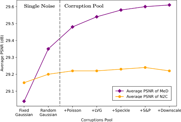
The influence of the size of the Corruption Pool on the performance of MeD and N2C [24] is demonstrated in Figure 5 (b). The experiments are started from only fixed Gaussian noise, then train on Gaussian noise with random sigma values. Finally, we expand the corruption pool from only Gaussian noise to more noise types and even with different types of down-scale and inpainting mask operations.
| Loss Hyperparameters for | Gaussian Noise | ||
| , , , | |||
| 31.18/ 0.8839 | 27.68/ 0.7765 | 25.74/ 0.7172 | |
| 31.04/ 0.8813 | 27.87/ 0.7788 | 25.86/ 0.7190 | |
| 30.85/ 0.8752 | 27.96/ 0.7794 | 25.92/ 0.7199 | |
| 31.31/ 0.8876 | 28.05/ 0.7810 | 26.01/ 0.7216 | |
| 31.29/ 0.8870 | 27.58/ 0.7659 | 24.29/ 0.6931 | |
| 31.20/ 0.8832 | 26.24/ 0.7391 | 23.78/ 0.6517 | |
| Training | Test | Noisy/ Clean | Noisy/ Noisy | Invariant Feature | ||||
| Schema | N2C [24] | DBD4 [13] | N2N [19] | N2S [5] | R2R [29] | LIR [11] | MeD | |
| Gaussian | 15 | 33.21/ 0.9194 | 33.17/ 0.9179 | 33.16/ 0.9175 | 32.88/ 0.9099 | 31.19/ 0.8752 | 29.29/ 0.8118 | 33.20/ 0.9181 |
| 25 | 28.04/ 0.7588 | 26.36/ 0.7473 | 26.56/ 0.7521 | 26.27/ 0.7456 | 23.51/ 0.5529 | 21.80/ 0.4802 | 29.80/0.8401 | |
| 50 | 19.89/ 0.3755 | 19.86/ 0.3741 | 19.68/ 0.3672 | 16.13/ 0.1978 | 16.09/ 0.2080 | 11.12/ 0.1217 | 23.51/ 0.5529 | |
| 75 | 17.16/ 0.2562 | 16.62/ 0.2314 | 14.59/ 0.1561 | 14.99/ 0.1642 | 14.09/ 0.1280 | 11.10/ 0.1042 | 20.47/ 0.3870 | |
| Gaussian | 15 | 30.69/ 0.8497 | 30.70/ 0.8478 | 30.80/ 0.8619 | 29.87/ 0.8267 | 28.15/ 0.7872 | 29.44/ 0.8011 | 30.88/ 0.8799 |
| 25 | 29.81/ 0.8140 | 29.63/ 0.8182 | 29.54/ 0.8256 | 29.54/ 0.8256 | 28.89/ 0.8099 | 28.95/ 0.7967 | 30.19/ 0.8218 | |
| 50 | 28.56/ 0.7721 | 28.32/ 0.7765 | 28.30/ 0.7490 | 28.19/ 0.7802 | 27.80/ 0.7547 | 28.02/ 0.7682 | 28.56/ 0.7835 | |
| 75 | 22.60/ 0.5877 | 22.47/ 0.6042 | 22.45/ 0.5759 | 21.69/ 0.5433 | 21.42/ 0.5881 | 20.25/ 0.5368 | 25.63/ 0.7372 | |
B.1 Hyperparameter Analysis
Prior to finalising the training procedure, we conducted experiments to analyse the impact of different hyperparameters associated with the loss terms in our model. Specifically, we tested varying the weighting factors , , and for the Noise Reconstruction loss, Scene Reconstruction loss, Cross Compose loss, and Mix Scene reconstruction loss, respectively. The analysis is shown in Figure 5 (a) and Table 8
Firstly, we conducted the experiment for analysing the value in Figure 5 (a). The orange (top) curve represents the performance of the optimal choice .
, and are tested from 0.5 to 1, with the best results obtained at , and .
Based on these experiments, we selected hyperparameters of , , , and for all denoising training in our work. This provides an optimal balance between the different objectives.
Appendix C Additional Denoising Evaluation
In this section, we present additional quantitative evaluations of our denoising results, which were not included in the main paper. The results are in Table 9 with additive Gaussian Noise, supplement to Table 1 in the main paper.
C.1 Generalisation on Unseen Noise Removal
To evaluate the generalisation ability of trained models on unseen noise removal, we conducted an additional experiment with more methods using only a single noisy image in Table 10. The results show that our method achieves comparable performance to state-of-the-art methods specially designed for Gaussian noise removal, and outperforms all compared methods on other noise types, while training only on the Gaussian noise. This further highlights the generalisation ability of our approach in handling unseen and unfamiliar noise distributions.
| Noise Type | DIP [32] | NAC [35] | S2S [30] | IDR [43] | Restormer [39] | MeD (Ours) |
| Gaussian, | 25.62/ 0.7017 | 27.13/ 0.7391 | 27.71/ 0.7622 | 28.52/ 0.8061 | 29.10/ 0.8250 | 28.45/ 0.8057 |
| Speckle, | 30.14/ 0.8574 | 31.55/ 0.8859 | 31.83/ 0.8980 | 28.62/ 0.8763 | 30.12/ 0.8557 | 33.48/ 0.9115 |
| S&P, | 28.62/ 0.7957 | 29.89/ 0.8741 | 30.57/ 0.9053 | 27.26/ 0.7544 | 23.09/ 0.6381 | 30.84/ 0.9135 |
| Average | 28.13/ 0.7849 | 29.52/ 0.8330 | 30.04/ 0.8552 | 28.13/ 0.8123 | 27.44/ 0.7729 | 30.92/ 0.8770 |
| Method | MAC (G) | Supervised | Trained with | SIDD [2] | PolyU [36] |
| Restormer [39] | 140.99 | ✓ | Real (SIDD) | 40.06/ 0.9601 | 36.38/ 0.9588 |
| NAFNet [8] | 63.6 | ✓ | Real (SIDD) | 40.31/ 0.9667 | 27.36/ 0.9225 |
| N2N [24] | 26.18 | ✗ | Real (SIDD) | 32.82/ 0.7297 | 36.22/ 0.9679 |
| N2S [5] | 26.18 | ✗ | Real (SIDD) | 30.98/ 0.6018 | 36.41/ 0.9721 |
| CVF-SID [28] | 77.86 | ✗ | Real (SIDD) | 34.71/ 0.9179 | 33.00/ 0.8768 |
| MM-BSN [40] | 339.46 | ✗ | Real (SIDD) | 37.37/ 0.9362 | 35.40/ 0.9484 |
| MeD (Ours) | 26.18 | ✗ | Synthetic (NP) | 35.81/ 0.8278 | 38.65/ 0.9855 |
| MeD (Ours) | 26.18 | ✗ | NP + SIDD | 37.52/ 0.9434 | 38.91/ 0.9894 |
C.2 Further Analysis on Real-world Generalisation
In the main paper, we have shown that our method generalises well to real-world scenarios when trained only on synthetic data. Moreover, here we conduct experiments on training with a real-world dataset (SIDD without GT), and report the test results on SIDD and PolyU in Table 11.
Analysis: Comparing Table 11 and Table 4 in the main paper, it shows that all methods have significant improvement in performance on SIDD after training on SIDD, but little improvement on PolyU.
Considering that collecting real data is expensive and sometimes infeasible compared to synthetic data and, as our following experiments show, generalising to new real datasets (real-to-real) is another issue (since the noise distributions are different), the model trained on synthetic noise data is more feasible and practical.
 |
 |
 |
 |
| Set5 “Bird” [7] | RCAN [44] | DASR [33] | MeD (Ours) |
| PSNR/SSIM | 34.89/ 0.9512 | 34.42/ 0.9364 | 36.66/ 0.9747 |


Appendix D More Application Exploration
D.1 Experiment on Image Super-resolution
Figure 6 and Figure 7 show the qualitative results of our method for ×3 and ×4 super-resolution on Set5 dataset [7], compared with RCAN [44] and DASR [33]. It shows that our method achieves better performance than these methods, by using a corruption pool that contains both noise and down-scaling process.
D.2 Experiment on Image Inpainting
Appendix E Datasets
We used five different datasets to train and evaluate the denoising methods: DIV2K [4], CBSD68 [26], SIDD [2], CC [27], and PolyU [36].
DIV2K:
DIVerse 2K resolution high-quality images [4] (DIV2K) contain 800 high-resolution images with a resolution of 2K or 4K.
To train our denoising method, we added different types and levels of noise to the DIV2K dataset.
CBSD68:
CBSD68 dataset [26] contains 68 colourful images with various levels of synthesising noise. These images were obtained from a range of sources, including natural scenes and synthetic images.
SIDD:
The Smartphone Image Denoising Dataset [2] (SIDD) is a large-scale real-world dataset containing 24,000 images captured by smartphone cameras in ten scenes with varying lighting conditions. The ground truth images for the SIDD dataset are provided along with the noisy images in the dataset.
CC:
Cross-Channel Image Noise Modeling [27] (CC) is another real-world dataset which contains 11 static scenes captured by three different consumer cameras. For each scene, it contains one temporal image and the precomputed temporal mean and covariance matrix data.
PolyU:
PolyU dataset [36] is comprised of 40 different scenes captured by cameras. It contains the original image corrupted by realistic noise and the ground truth version which is obtained by averaging multiple exposures to remove the noise.
We also used Set5 dataset [7] and Set11 [16] to evaluate the super-resolution and image inpainting performances.
Set5 dataset:
We use Set5 dataset [7] for super-resolution task.
The Set5 dataset [7] consists of 5 high-quality images with different contents, including “baby”, “bird”, “butterfly”, “head”, and “woman”. Each of the images in the Set5 dataset has a magnifying factor of 2, 3, or 4, allowing us to evaluate the performance of our image super-resolution model across a range of magnification factors.
Appendix F Synthesising Noisy Data and Downsampling Corruptions
We utilise the Pillow library222https://pillow.readthedocs.io/en/stable/ in Python to synthesise noisy data and perform downsampling corruptions.
F.1 Synthesising Noise
To evaluate the performance of our proposed algorithm, we synthesised noisy images using several types of noise models, including Gaussian, Local Variance Gaussian, Poisson, Speckle, and Salt-and-Pepper.
Remark: The original pixel value at position in the image can be notated as and the noisy pixel value can be notated as .
Gaussian Noise: Gaussian noise is a type of additive noise that is commonly found in digital images. It is modelled as a normal distribution with zero mean and a standard deviation . To synthesise Gaussian noise, we added Gaussian-distributed noise to the original image. Specifically, we added Gaussian noise with zero mean and standard deviation to each pixel of the input image, where was set to 10. The noisy pixel value is given by:
| (17) |
is a random variable generated from a Gaussian distribution with zero mean and standard deviation .
Local Variance Gaussian Noise: Local Variance Gaussian noise is a variant of Gaussian noise that takes into account the local variance of the image. In this case, we added Gaussian noise with different standard deviations to different local regions of the input image to achieve more realistic noise patterns. Specifically, the standard deviation of Gaussian noise for each pixel was calculated based on the local variance of its neighbouring pixels. The noisy pixel value is given by:
| (18) |
where is a random variable generated from a Gaussian distribution with zero mean and standard deviation , which is calculated as:
| (19) |
where is the local variance of the image at pixel , and is a scaling factor that determines the strength of the noise.
Poisson Noise: Poisson noise is a type of noise that arises from the random nature of photon arrival in digital images. It is modelled as a Poisson distribution with parameter . To synthesise Poisson noise, we first modelled the image as a Poisson process and then generated noisy pixels based on this model. Specifically, the noisy pixel value is given by:
| (20) |
where is the original pixel value at position , is the mean value of the Poisson distribution, and is a random variable generated from a Poisson distribution with mean .
Speckle Noise: Speckle noise is a type of multiplicative noise that is commonly found in ultrasound and radar images. It is modelled as a multiplicative noise with a uniform distribution between 0 and 1. To synthesise speckle noise, we multiplied each pixel of the original image with a random value drawn from a uniform distribution between 0 and 1. Specifically, the noisy pixel value is given by:
| (21) |
where is a random variable drawn from a uniform distribution between 0 and 1.
Salt-and-Pepper Noise: Salt-and-pepper noise is a type of impulse noise that occurs when some pixels in the image are replaced with the maximum or minimum pixel value. It is modelled as a random process that replaces a certain percentage of the pixels in the image with either the maximum or minimum pixel value. Specifically, the noisy pixel value can be calculated as follows:
| (22) |
where and are random variables that model the presence of salt-and-pepper noise, respectively. They are defined as follows:
| (23) |
| (24) |
where is a random variable that takes the value 1 with probability p and the value 0 with probability .
Note that and are only added to the pixel value with the respective set probabilities and . Therefore, the total percentage of pixels affected by salt and pepper noise is .
F.2 Downscale Corruption
The down-scale corruption contains down-scale interpolation, including Bicubic, Lanczos, Bilinear and Hamming. We use OpenCV-Python for the down-scaling process.
Appendix G Additional Qualitative Results
The following figures show the denoising comparison on both synthetic noise removal (Figure 9 – Figure 18) and denoising real noise data (Figure 19 – Figure 26).