Multilevel lattice-based kernel approximation for elliptic PDEs with random coefficients
Abstract
This paper introduces a multilevel kernel-based approximation method to estimate efficiently solutions to elliptic partial differential equations (PDEs) with periodic random coefficients. Building upon the work of Kaarnioja, Kazashi, Kuo, Nobile, Sloan (Numer. Math., 2022) on kernel interpolation with quasi-Monte Carlo (QMC) lattice point sets, we leverage multilevel techniques to enhance computational efficiency while maintaining a given level of accuracy. In the function space setting with product-type weight parameters, the single-level approximation can achieve an accuracy of with cost for positive constants depending on the rates of convergence associated with dimension truncation, kernel approximation, and finite element approximation, respectively. Our multilevel approximation can achieve the same accuracy at a reduced cost . Full regularity theory and error analysis are provided, followed by numerical experiments that validate the efficacy of the proposed multilevel approximation in comparison to the single-level approach.
1 Introduction
Kernel-based interpolation using a quasi-Monte Carlo (QMC) lattice design was first introduced in [48], where the authors analysed splines constructed from reproducing kernel functions on a lattice point set for periodic function approximation. They found that the special structure of a lattice point set coupled with periodic kernel functions led to linear systems with a circulant matrix that were able to be solved efficiently via the fast Fourier transform (FFT). The recent paper [23] applies kernel interpolation for approximating the solutions to partial differential equations (PDEs) with periodic random coefficients over the parametric domain. In this paper, we seek to enhance the kernel-based approximation method for estimating PDEs over the parametric domain by leveraging multilevel methods [17].
We are interested in the following parametric elliptic PDE
| (1.1) | |||||
where the physical variable belongs to a bounded convex domain , for or , and
is a countable vector of parameters. It is assumed that the input field in (1.1) is represented by the periodic model introduced recently in [24], which is periodic in and given by the series expansion
| (1.2) |
Here , where each is independent and uniformly distributed on . The functions are known and deterministic such that for all . Additional requirements on will be introduced later as necessary.
The goal is to approximate efficiently the solution in both and simultaneously. We will follow a similar method to [23], where the approximation is based on discretising the spatial domain using finite elements and applying kernel approximation over the parametric domain based on a lattice point set. This paper introduces a new multilevel approximation that spreads the work over a hierarchy of finite element meshes and kernel interpolants so that the overall cost is reduced.
The solution to (1.1) with the coefficient given by (1.2) lies in a periodic function space (with respect to the parametric domain) equipped with a reproducing kernel . Given evaluations on a lattice point set , the solution can be approximated over using a kernel interpolant given by
| (1.3) |
where is the kernel interpolation operator on . The coefficients for are obtained by solving the linear system associated with interpolation at the lattice points via FFT. Combining (1.3) with a finite element discretisation leads to an approximation of over . This is the method employed by [23], which we will refer to as the single-level kernel interpolant (see also Section 2.6 for details).
To introduce the multilevel kernel approximation, consider now a sequence of kernel interpolants , for , based on a sequence of embedded lattice point sets with nonincreasing size and a sequence of nested finite element approximations for , where becomes increasingly accurate (and thus has increasing cost) as increases. Omitting the and dependence, the multilevel kernel approximation with maximum level is given by
| (1.4) |
The motivation of such an algorithm is to reduce the overall computational cost compared to the single-level method while achieving the same level of accuracy. The cost savings come from interpolating the difference , which converges to 0 as increases, thus requiring an interpolation approximation with fewer points to achieve a comparable level of accuracy. Indeed, as will be demonstrated later, to achieve an accuracy of with the single-level approximation in the function space setting with product-type weight parameters, the computational cost is for positive constants depending on the rates of convergence for dimension truncation, kernel approximation, and finite element approximation, respectively; whereas for the multilevel approximation, the cost is reduced to . The main contribution of this work is to introduce the multilevel kernel approximation along with a full error and cost analysis.
Parametric PDEs of the form (1.1) can be used to model steady-state flow through porous media and have been thoroughly studied in uncertainty quantification literature (see e.g., [2, 4, 5, 6, 44]). QMC methods have achieved much success in tackling parametric PDE problems, including evaluating expected values of quantities of interest (see, e.g., [13, 14, 19, 33, 34]), as well as density estimation (see [14]). The two most common forms of random coefficient are the uniform model (see e.g., [6, 33, 34]) and lognormal model (see e.g., [2, 4, 44]), and as an alternative, the periodic model (1.2) was introduced in [24] to exploit fast Fourier methods.
Multivariate function approximation is another area where QMC methods have recently been successful. One example is trigonometric approximation in periodic spaces, where lattice rules are used to evaluate the coefficients in a finite (or truncated) Fourier expansion (see e.g., [1, 26, 27, 28, 29, 35, 36]). Fast component-by-component algorithms for constructing good lattice rules for trigonometric approximation in periodic spaces were presented and analysed in [7, 8].
There has also been research on kernel methods for approximation such as radial basis approximation for interpolating scattered data, signal processing, and meshless methods for solving PDEs (see e.g., [11, 21, 37, 40, 45, 46]). Approximation in using kernel interpolation on a lattice in a periodic setting was first analysed in [48], which also highlighted the advantage that linear systems involved can be solved efficiently via FFT; see also [47] for the case. The paper [23] introduced single level kernel interpolation with lattice points for parametric PDEs and also provided a full analysis of the error on .
Multilevel methods were first introduced in [22] for parametric integration and then developed further in [15, 16] for pricing financial options by computing the expected value of a pay-off depending on a stochastic differential equation utilising paths simulated via Monte Carlo (MC). These papers showed that the overall computational cost of the multilevel estimator was lower than that of the direct estimate at the same level of error. Multilevel MC methods were extended to multilevel QMC in [18]. Subsequently, multilevel methods with MC and QMC have been successfully used in several papers to compute expectations of quantities of interest from parametric PDEs (see e.g., [2, 5, 13, 34]). The paper [43] employed a similar multilevel strategy to approximate the PDE solution on , where instead of using kernel interpolation on the parameter domain (as in this paper) they used sparse grid stochastic collocation.
To the best of our knowledge, this paper is the first to use a multilevel approach with a QMC method to approximate the solution of a PDE as a function over both the spatial and parametric domains.
The structure of the paper is as follows. Section 2 summarises the problem setting and essential background on dimension truncation, finite element methods and kernel interpolation. Section 3 introduces the multilevel kernel approximation alongside a breakdown of the error and the corresponding multilevel cost analysis. Section 4 includes the regularity analysis required for the error analysis presented in Section 5. Practical details on implementing our multilevel approximation are covered in Section 6. Finally, Section 7 presents results of the numerical experiments. Any technical proofs not detailed in the main text are provided in the appendix.
2 Background
2.1 Notation
Let with be a multi-index, and let and . Define to be the set of multi-indices with finite support, i.e., Multi-index notation is used for the parametric derivatives, i.e., the mixed partial derivative of order with respect to is denoted by .
For , we define and interpret to be for all (i.e., comparison between indices is done componentwise). For a given sequence , we define .
The Stirling numbers of the second kind are given by
| (2.1) |
The notation means that there exists some such that , and means that there exists constants such that and .
For , we define the -norm on by
Furthermore, note that all functions in this paper are measurable, so by Fubini’s Theorem we can swap the order of the integrals to give .
2.2 Parametric variational formulation
Let denote the usual first order Sobolev space of functions on that vanish on the boundary, with associated norm Multiplying both sides of (1.1) by a test function and then integrating with respect to , using the divergence theorem, yields the variational equation: find such that
| (2.2) |
where , with denoting the dual space of , and is the parametric bilinear form defined by
The inner product is extended continuously to the duality pairing on .
The variational problem (2.2) is subject to the same assumptions as in [24]:
-
(A1)
and ,
-
(A2)
there are positive constants and such that for all and ,
-
(A3)
for some ,
-
(A4)
and ,
-
(A5)
, and
-
(A6)
the physical domain , where or , is a convex and bounded polyhedron with plane faces.
Here is the Sobolev space with essentially bounded first order weak derivatives, equipped with the norm . For the new multilevel analysis, we will also require additional assumptions:
-
(A7)
for some , and
-
(A8)
.
We additionally define
| (2.3) |
2.3 Dimension truncation
To approximate in , the infinite-dimensional parameter domain must be first truncated to a finite number of dimensions . This is done by setting for , where we define the truncated parameter , or equivalently by truncating the coefficient expansion (1.2) to terms. The dimension-truncated solution is denoted by and it is obtained by solving the variational problem (2.2) at . With a slight abuse of notation we treat as a vector in the -dimensional parameter domain .
The dimension-truncated problem is subject to all the same assumptions as the variational problem (2.2) (i.e., Assumptions (A(A0))–(A(A6)) hold), hence, the a priori bound (2.4) and regularity bound (2.5) also hold here. Additionally, we have from [23, Theorem 4.1] that
| (2.6) |
where the implied constant is independent of and .
2.4 Finite element methods
The solution to the PDE (1.1) will be approximated by discretising in space using the finite element (FE) method. We consider piecewise linear FE methods, however, the multilevel method can be applied using more general discretisations. Denote by the space of continuous piecewise linear functions on a shape-regular triangulation of with mesh width and . For , the FE approximation of from (2.2) is obtained by finding such that
| (2.7) |
The FE basis functions for the space are denoted by , , and the FE approximation with coefficients given by can be represented as
| (2.8) |
Since , the a priori bound (2.4) and the regularity bound (2.5) also hold for the FE approximation , as well as for FE approximation of the dimension-truncated solution, denoted .
From [23, Theorem 4.3], we have that under Assumptions (A(A0)), (A(A0)), (A(A0)), (A(A0)), and (A(A6)), the error of FE approximation satisfies
| (2.9) |
where the implied constant is independent of , and . By Galerkin orthogonality, the FE error is orthogonal to , i.e.,
| (2.10) |
We also define to be the identity operator and to be the parametric FE projection operator onto , which is defined for some by
| (2.11) |
The approximation is the projection of onto , i.e., , and by the definition of a projection on .
2.5 Lattice-based kernel interpolation
The solution will be approximated via kernel interpolation in the dimension-truncated parametric domain . Consider the weighted Korobov space , which is the Hilbert space of one-periodic functions defined on with absolutely convergent Fourier series and square-integrable mixed derivatives of order . We restrict to be an integer smoothness parameter111In general, need not be an integer (e.g., see [23, 42]), however, to have a simple, closed-form representation of the reproducing kernel and norm we restrict ourselves to integer . and include weight parameters that model the relative importance of different groups of parametric variables. The space is a reproducing kernel Hilbert space, equipped with the norm
| (2.13) |
where and . The reproducing kernel for this space, , is given by
where is the Bernoulli polynomial of degree .
Consider a set of lattice points defined by
where is a generating vector with components in that are coprime to . For , the lattice-based kernel interpolant (defined using function values of evaluated at the points ) is given by
| (2.14) |
such that for all . The generating vector is obtained using a component-by-component (CBC) construction algorithm similar to those described in [7, 8, 23], where components of the vector are selected to minimise a bound on the worst-case error of approximation using the kernel method. To ensure that interpolates at the lattice points, the coefficients are obtained by solving the linear system
| (2.15) |
with , and .
Due to the periodic and symmetric nature of the kernel, along with the properties of the lattice point set, the elements of satisfy
for . This implies that is a symmetric, circulant matrix uniquely determined by its first column and can be diagonalised via FFT at cost . The kernel only needs to be evaluated at lattice points, since the first column is symmetric about its midpoint, and the linear system (2.15) can be solved after diagonalising using the FFT.
A bound on the approximation error for the kernel interpolation of using a CBC generated lattice point set is given in [23, Theorem 3.3], which states that
| (2.16) |
for all with . Here is the identity operator, is the Riemann zeta function defined by , and is the Euler totient function. Note that the original theorem presented in [23] requires the number of points to be prime, however, using [30, Theorem 3.4] the result above has been extended to non-prime .
There are weight parameters , too many to specify individually in practice. Therefore, special forms of weights have been considered, including:
-
•
Product weights: for some positive sequence ;
-
•
POD (“product and order dependent”) weights: for positive sequences and ;
-
•
SPOD (“smoothness-driven product and order dependent”) weights: for positive sequences and .
The error bound (2.16) holds for all forms of weights, but the computational cost differs, see the next subsection.
2.6 Single-level kernel interpolation for PDEs
Lattice-based kernel interpolation was first applied to PDE problems in [23]. Denoting the dimension-truncated FE solution of (2.2) by , the estimate (2.16) can be applied to the single-level kernel interpolant (see [23, Theorem 4.4]) to obtain
| (2.17) |
for all , where
In [23], the weights are chosen to ensure the constant can be bounded independently of dimension . Different forms of weights (SPOD, POD, product) achieve dimension independent bounds with some concessions on the rate of convergence.
The single-level kernel interpolation methodology from [23] is summarised below:
- 1.
-
2.
Evaluate the coefficient (1.2) at each lattice point and FE node to set up the stiffness matrix at the cost .
- 3.
-
4.
Solve the circulant linear system (2.15) for coefficients of the interpolant for every FE node at the cost .
The total cost of construction for the single-level interpolant is therefore
| (2.18) |
There is a pre-computation cost (varies with the form of weights) associated with the CBC construction of the lattice generating vector . There is also a post-computation cost to assemble the approximation.
From [23], the error satisfies
see (2.6), (2.9), (2.17), with , , and for . The cost can now be expressed in terms of the error as follows. We demand that each of the three components of the error is bounded above and below by multiples of , i.e., , and . It follows that there exists such that , which gives since , and therefore . Assuming that and treating as a constant, the cost (2.18) can be bounded further by
| (2.19) |
In the case of product weights, we have and .
3 Multilevel kernel approximation
Consider a sequence of conforming FE spaces , where each corresponds to a shape regular triangulation of with mesh width and . Recall that . Then for , we denote the dimension-truncated FE approximation in the space by .
For a maximum level and setting , the multilevel kernel approximation is given by (1.4), where is a sequence of interpolation operators such that each is a real-valued kernel interpolant based on lattice points as defined in Section 2.5. The interpolants are ordered in terms of nonincreasing accuracy, or equivalently, nonincreasing numbers of interpolation points, i.e., . The intuition is that the magnitude of decreases with increasing , thus requiring fewer interpolation points to achieve reasonable accuracy.
We assume that the FE solution at each level is approximated with increasingly fine meshes corresponding to mesh widths (i.e., the approximation increases in accuracy as the level increases), so that approximations using large values of are compensated by coarser FE meshes, thus moderating the cost. To simplify the ML algorithm, we additionally assume that the FE spaces are nested, i.e., for . If non-nested FE spaces are used, a “supermesh” (the mesh corresponding to the space spanned by the basis functions of both and ) must be considered, which adds to the computational cost (see e.g., [9, 10, 12]).
Similarly, we assume the lattice points on each level are nested (i.e., the points used on each level form a subset of the points used on level ), which can be achieved using an embedded lattice rule (see [30]). Thus, the space spanned by the kernel basis functions on level is a subspace of the one spanned by the kernel basis functions on level . This proves to be advantageous since the generating vector for the lattice only needs to be constructed once and FE evaluations can be reused between levels, e.g., evaluations used to compute can be reused to compute .
To compute the multilevel kernel approximation, on each level , we compute the -point interpolant of the difference of a FE approximation on a fine mesh, , and a coarse mesh, . As a result, the final approximation is not a direct interpolation of the solution , and thus will be referred to exclusively as the multilevel kernel approximation.
3.1 Error decomposition for multilevel methods
The multilevel kernel approximation error can be expressed as (omitting the dependence on and )
where denotes the identity operator, and we define . Following the methodology of [23], we take the norm and norm, then use the triangle inequality to obtain the error estimate,
| (3.1) |
The first term in (3.1) is often referred to as the bias in multilevel literature, which can be further separated into a dimension truncation error and a FE error
| (3.2) |
where the two components can be bounded using (2.6) and (2.9). The bias is controlled by choosing and as necessary to obtain a prescribed error. The second term in (3.1) is the error associated with the multilevel scheme, which is controlled by the choice of interpolation points and the fineness of the FE mesh at each level.
3.2 Cost analysis of multilevel methods
The cost of constructing the multilevel kernel approximation is similar to the single-level interpolant, except now the cost is “spread” over multiple levels. Recall from Subsection 2.6 that the total cost of construction for the single-level kernel interpolant is given by (2.18). For the multilevel algorithm, the total cost is from
-
1.
evaluating the kernel functions for the full lattice point set, ,
-
2.
then, for each level with ,
-
(a)
evaluating the coefficient (1.2) at each lattice point and FE node to set up the stiffness matrix, ,
-
(b)
solving for the FE solution at each lattice point, , and
-
(c)
solving the linear system for coefficients of the interpolant at every FE node, .
-
(a)
Since the lattice points are nested, the total cost of computation is
| (3.3) |
Since kernel functions only need to be evaluated for each lattice point once and can be reused at each level as necessary, this cost, given by , is independent of and is outside the summation. For details on practical implementation, see Section 6.
3.3 Abstract complexity analysis
Theorem 1 below is an abstract complexity theorem for the error and cost of our multilevel approximation. It specifies a choice of , , and for such that the total error of approximation can be bounded by some given . Assumption (M(M2)) is motivated by the bias split (3.2) together with (2.6) and (2.9), and is chosen to balance the two terms. Assumption (M(M2)) is motivated by the cost estimate (3.3), where is treated as constant, and a bound on is assumed to simplify the cost. The error analysis in Section 5 will justify Assumption (M(M2)) with precise values of the relevant constants.
Theorem 1.
Proof.
Substituting Assumptions (M(M2)) and (M(M2)) into (3.1) gives the error bound
Choosing to balance the two components of error in Assumption (M(M2)), i.e., setting , the bound further simplifies to
| (3.5) |
where the implied constant depends on a factor .
We require that , which holds if each of the two terms in (3.5) is bounded by . So from the first term we choose such that , yielding the conditions . Taking the smallest allowable value of with the ceiling function, we obtain
| (3.6) |
To ensure so that we are not in the trivial single-level case, we require that the value inside the ceiling function is positive, giving the condition . For the second term in (3.5), we demand that
| (3.7) |
Since we have assumed that , which follows from desiring , Assumption (M(M2)) simplifies to
| (3.8) |
If for all , then, using , the cost (3.8) can be bounded by
| (3.9) |
where the first term represents a setup cost and the second term is the multilevel cost.
We now proceed to choose by minimising the multilevel cost term in (3.9) subject to the constraint (3.7), with equality instead of . We will later verify that the condition is indeed true. The Lagrangian for this optimisation is
where is the Lagrange multiplier and for are continuous variables. This gives us the following first-order optimality conditions
| (3.10) | ||||
| (3.11) |
Rearranging (3.10) gives for , noting that the right-hand side is independent of . Thus, we have for , so
| (3.12) |
Substituting (3.12) into (3.11) gives
| (3.13) |
To obtain integer values for , we define
| (3.14) |
Since , the bound (3.7) continues to hold for this choice of .
Clearly, as required. We now verify that . Since , we have from (3.13), and therefore
where we loosely overestimated the geometric series in (3.13) by taking times the largest possible term with absolute value in the exponent, and then used and from (3.6). Thus . On the other hand, we have and so . Hence we have as required. We conclude that the results from the optimisation with respect to the simplified cost function (3.9) can be applied to the multilevel problem with cost given by Assumption (M(M2)).
We now verify that the cost satisfies (3.4) by substituting , , (3.13), , and into (3.9), resulting in
where the implied constant includes a factor , and we used
The final case in the cost (i.e., when ) is split into two cases based on which of the two terms dominates, resulting in the four cases in (3.4). ∎
The third case in (3.4) becomes obsolete when , i.e., when we have product weights. In this scenario, to achieve an accuracy , the cost for the multilevel approximation is , compared to for the single-level approximation. This multilevel cost is near-optimal, since the cost of a single FE evaluation at the finest level is and the cost of interpolation at level at a single node is .
We note that when , we may encounter the scenario where the single-level cost and multilevel cost have the same order. This occurs when the setup cost in Assumption (M(M2)) dominates, either due to a large dimension or because the contribution to the cost from the FE solves is relatively small due to fast convergence in FE error (i.e., is large). Such cases are exceptional, and it would be unnecessary to consider a multilevel approach in these situations.
4 Parametric regularity analysis
Analysis of the multilevel kernel approximation error for parametric PDEs requires bounds on the mixed derivatives with respect to both the physical variable and the parametric variable simultaneously. The proofs of all parametric regularity lemmas in this section are given in Appendix II.
The following lemma provides a bound on the Laplacian of the derivatives (with respect to the parametric variables) of the solution to (2.2). It shows that and its derivatives with respect to possess sufficient spatial regularity to establish estimates for the FE error. Recall that Stirling numbers are defined by (2.1).
Lemma 2.
The following lemma gives a bound on the derivatives with respect to the parametric variables of the FE error in .
Lemma 3.
We are interested in regularity estimates with respect to the norm. Thus, Lemma 4 presents the bound on the norm of the derivatives of FE error obtained using a duality argument.
5 Multilevel error analysis
We are now ready to derive an estimate for the final component of the error in (3.1).
5.1 Estimating the multilevel FE error
Clearly, for any that is a function solely of . Then, taking the -norm and using the triangle inequality, we have from (2.16) the following pointwise bound for some ,
| (5.1) |
where
| (5.2) |
It then follows that the sum over in (3.1) can be bounded by
| (5.3) |
where we separate out the term as it is simply the standard single-level kernel interpolation error for which the bound (2.17) applies. Combining (5.1) and (5.2) with the triangular inequality gives the last line.
Therefore, we seek to estimate the individual finite element error terms in the above expression to estimate the full multilevel kernel approximation error.
Theorem 5.
Proof.
From the definition of the norm of given in (2.13) and the Cauchy-Schwarz inequality, it follows that for any ,
Now, taking the -norm with respect to and applying the Fubini-Tonelli theorem gives
In the step with , we applied Lemma 4 for each with given by for and for , and denotes the multi-index with for all , with . The implied constant is independent of . Taking the square-root completes the proof. ∎
5.2 Choosing the weight parameters
We now choose the weights to minimise and select to obtain the best possible convergence rate, while ensuring that is bounded independently of .
Theorem 7.
Suppose that Assumptions (A(A0))–(A(A6)) hold. The choice of weights
| (5.5) |
for , , and , minimise given in (6). Here is defined in (2.3). In addition, if we take and , then can be bounded independently of dimension . Thus, the multilevel kernel approximation of the dimension-truncated FE solution of (2.2) satisfies
| (5.6) |
where we define , and the implied constant is independent of .
Proof.
The proof of this theorem follows very closely to that of [23, Theorem 4.5]. We seek to choose weights to bound the constant independently of dimension. Applying [33, Lemma 6.2] to (6), we find that the weights given by (5.5) minimise .
Defining a new sequence for , we can write, for ,
where . The cardinality of is . Then, following [23], the upper bound (5.7) can be further bounded above by
| (5.8) |
Now following from Assumption (A(A6)), we know , so we choose such that which gives . Then
provided that , which can be ensured by choosing . This condition can be satisfied by taking .
To show the full series (5.8) converges we perform the ratio test with the terms of the series given by . This shows that can be bounded from above independently of dimension since
where the inequality results from using the fact that for .
Remark 8.
The recent paper [41] demonstrates that it is possible to achieve double the convergence rate of the kernel approximation error for functions that are sufficiently smooth, by leveraging the orthogonal projection property of the kernel interpolant, using a method reminiscent of the Aubin-Nitsche trick. The theory from [41] can be directly applied to our theoretical results, i.e., one should expect a convergence rate of rather than the as implied by (2.16), since the analytic nature of the solution of (2.2) with respect to implies that for all . However, if we impose restrictions to ensure dimension independence of the constant , then we cannot simply double the convergence rate in (5.6). Instead, the convergence rate for the QMC error determined in Theorem 7 will remain unmodified, while the choices of and will change. We now choose and , which means that could now be selected to be smaller than before whilst maintaining the same rate of convergence and dimension independence of the constant.
The main result for total error of approximation using the multilevel kernel approximation method is presented below.
Theorem 9.
Proof.
Remark 10.
CBC construction with weights of the form (5.5) are too costly to implement. Following [23], it can be shown that Theorem 9 continues to hold for the SPOD weights
However, these SPOD weights still come with a quadratic cost in dimension when evaluating the kernel basis functions to construct the approximation compared to the linear cost of product weights. Instead, the paper [25] proposes serendipitous product weights, whereby the order-dependent part of the weights is simply omitted, giving in our case
| (5.9) |
For these weights, the upper bound on the error of the kernel approximation will continue to have the same theoretical rates of convergence seen in Theorem 9, although the implied constant will no longer be independent of .
The paper [25] demonstrates that serendipitous product weights offer comparable performance to SPOD weights for easier problems and superior performance in problems where SPOD weights may fail completely. A possible explanation is that the SPOD weights derived from theory may be poorer due to overestimates in the bounds. A second, more practical explanation is that the magnitude of SPOD weights substantially increases as dimension grows which leads to larger, more peaked kernel basis functions. The resulting approximations using these basis functions tend to also be very peaked, resulting in a less “smooth” approximation. It is worth noting that integration problems are more robust to overestimates that may affect the quality of weights, as the weights do not directly appear in the computation of the integral. This is not true for the kernel approximation problem where the weights appear explicitly in the kernel basis functions.
6 Implementing the ML kernel approximation
In this section, we outline how to compute efficiently the multilevel approximation for the PDE problem using a matrix-vector representation of (1.4). Throughout we consider a fixed truncation dimension and so omit the superscript .
First, we outline how to construct the single-level kernel interpolant for the PDE problem. As in [23], the single-level kernel interpolant applied to the FE approximation of the PDE solution is given by (2.14) with , for . Each kernel interpolant coefficient is now a FE function, which we can expand using the FE basis functions , with , to write
| (6.1) |
To enforce interpolation for the FE solution, we equate the coefficients of the FE functions in (2.8) and (6.1) at each lattice point , leading to the requirement
Thus, the coefficients are the solution to the matrix equation
where , and is an matrix of the FE nodal values at the lattice points.
Next we present a similar matrix-vector representation for the multilevel kernel approximation (1.4). Since we are using an embedded lattice rule, is a factor of and the point sets across the levels are embedded, with an ordering such that
| (6.2) |
It follows that and the kernel matrices for each level are nested with the same structure.
Since the FE spaces are also nested, we can expand the difference on each level in the FE basis for
| (6.3) |
where and are the FE coefficients for after (exact) interpolation onto .
Similar to (6.1), the kernel approximation on level is
| (6.4) |
and we now choose the coefficients such that (6.4) interpolates the difference (6.3) at each lattice point . This leads to matrix equations
| (6.5) |
where now each coefficient matrix is , is the matrix of FE coefficients at the lattice points for level , and is the matrix of FE coefficients for interpolated onto then evaluated at the lattice points for level .
To obtain each coefficient matrix , we exploit the circulant structure of kernel matrices to solve the linear systems (6.5) using FFT. As a result, we only require the first column of each and furthermore, since the lattice points are nested as in (6.2), we obtain this column by taking every th entry (starting from the first) of the first column of . Similarly, since the FE spaces are nested we obtain for using the FE matrix from the previous level. Specifically, we take every th row of then interpolate it onto to give . This procedure is given in Algorithm 1.
On completion of Algorithm 1, we have a collection of coefficient matrices that we can use to compute , using (1.4) and (6.4), to approximate the PDE solution at any . By using the embedded property of the lattice points and the local support of the FE basis, we can evaluate efficiently with cost as we explain below.
We can write (6.4) as
Effectively, for each , we compute the sum over in (6.4) by “interpolating in space” along the columns of to get a kernel coefficient vector at , denoted . Since the FE basis functions are locally supported, there will be a small number of indices in (6.4) such that is nonzero. Multiplying the corresponding columns by and summing them up then gives at a cost of . In the second equality above we used the embedded property of the lattice points (6.2) to write this as a sum over the entire lattice point set. The indicator function accounts for the extra terms that were added.
Summing over gives a single kernel coefficient vector ,
at a cost . Since the points are embedded and hence, the total cost to construct the kernel coefficient vector is .
Similarly, we store all of the kernel evaluations at anchored at each of the lattice points in a single vector , which costs where depend on the structure of the kernel and are specified in Section 2.6.
Finally, the ML kernel approximation of is computed by the product
Combining the costs above leads to a total cost of evaluating of .
7 Numerical experiments
In this section, we present the results of numerical experiments conducted using the high performance computational cluster Katana [38].
7.1 Problem specification
The parametric PDE.
We consider the spatial domain with source term . For the parametric coefficient defined in (1.2), we choose and
where is a scaling parameter to vary the magnitude of the random coefficient, and is a decay parameter determining how quickly the importance of each random parameter decreases. The factor is included for easier comparison to the experiments in [23] and [25]. For this choice, the bounds on the coefficient assumed in (A(A0)) are given by and . Thus, from (2.3) we have
Assumptions (A(A0)) and (A(A6)) hold provided that and . Having chosen , we can set .
We will present numerical results for two choices of parameters: and , with the first being easier than the second, and consider the truncated parametric domain , i.e., .
Smoothness, weights, and CBC construction.
The smoothness parameter of the kernel is fixed as . We refrain from using higher values of to avoid stability issues in inaccurate eigenvalue computation via FFT in double precision. Issues in double precision computations arise even for small values of and relatively small , necessitating the use of arbitrary-precision computing (see e.g., [31]).
Convergence and cost.
According to (2.17) and Theorem 6, and ignoring the dependence of the constants on (which is fixed here), we have theoretically convergence in Assumption (M(M2)) of Theorem 1 with . As explained in Remark 8, since the PDE solution has a higher smoothness order than , the theoretical convergence rate doubles to .
Recall that the computational cost to achieve an error for the single-level approximation is (2.19), and for the multilevel approximation it is (3.4). Our spatial domain is the unit square, so . The FE convergence rate in Assumption (M(M2)) of Theorem 1 is determined by Theorem 6 to be , which also applies for the single-level FE error as indicated by (2.9). Since the serendipitous weights (5.9) are product weights, we have . With a fixed dimension , we may informally set and in Theorem 1. The third case in (3.4) is not relevant when using product weights. Hence, we obtain the theoretical cost bounds
| (7.1) |
7.2 Diagnostic plots
FE.
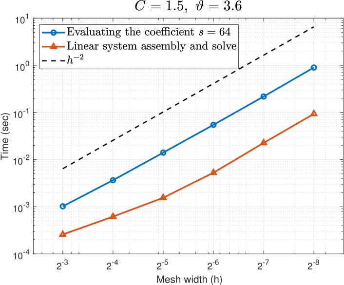
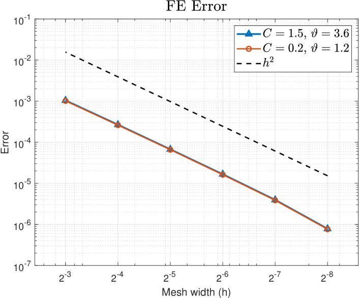
Figure 1 plots the computational cost, measured by CPU time in seconds, of assembling and solving the FE linear system required to obtain the PDE solution, and the FE error for mesh widths with respect to the reference solution with mesh width and . We use lattice points for the integral over , and the norm is computed exactly from the FE coefficients. We observe an error convergence rate of and a cost of , demonstrating that indeed and in Assumptions (M(M2)) and (M(M2)) of Theorem 1.
Dimension truncation.
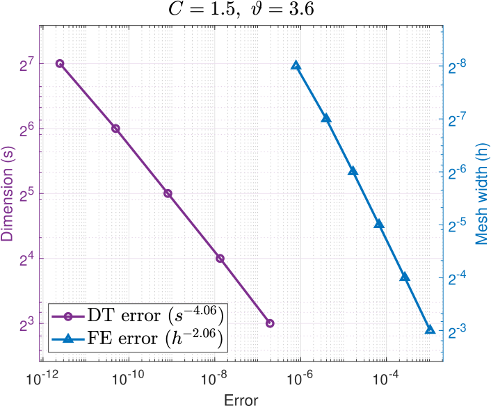
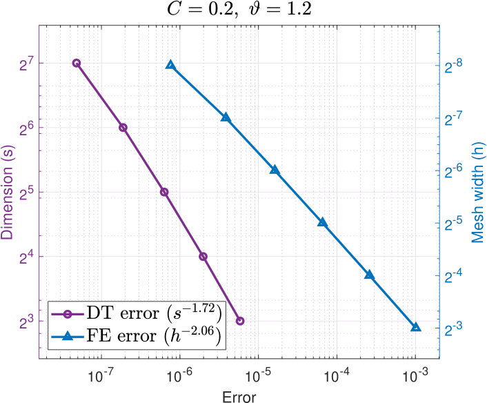
For and reference values and , we compute the error using lattice points. In Figure 2, on the horizontal axis, we overlay the dimension truncation errors with the FE errors for , with the vertical axis on the left in terms of (purple circles), and on the right in terms of (blue triangles). (The relative slope between the overlaid plots is arbitrary.) We observe convergence (c.f. Assumption (M(M2)) of Theorem 1) with for the easier problem , and for the harder problem . For both problems with we obtain dimension truncation errors much less than , i.e., smaller than all the FE errors with in Figure 1.
Single-level kernel interpolation.
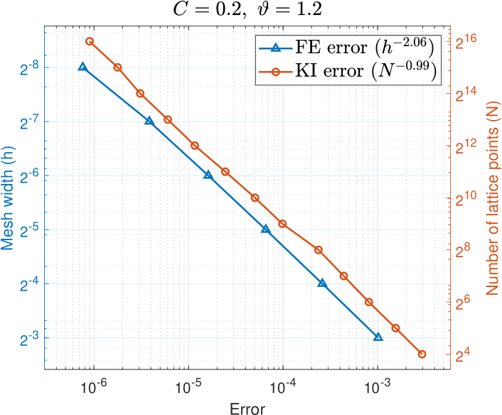
Following [23], we use an efficient formula to estimate the single-level kernel interpolation error
where is a sequence of Sobol′ points, is a sequence of lattice points, with , , , and . In Figure 3, on the horizontal axis, we overlay the interpolation errors with the FE errors for , with the vertical axis on the left in terms of (blue triangles), and on the right in terms of (red circles). We observe convergence for the easier problem , and for the harder problem .
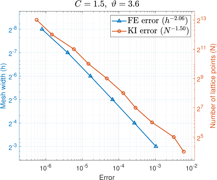
| SL | 0 | 1 | 2 | 3 | 4 | 5 | ||
|---|---|---|---|---|---|---|---|---|
We use Figure 3 to decide how to match the FE mesh width to the number of lattice points so as to give comparable errors. For each from the FE error data point in Figure 3, we trace upward to maintain the same error and look for the nearest interpolation error data point in order to find a matching with a similar error. (Note that the relative slope between the overlaid plots is arbitrary and does not affect the outcome.) This yields the pairings for the single-level kernel interpolant for the two problems in Table 1. We will also use Table 1 to form the pairings for our multilevel kernel approximation below. Notice the reverse labeling in Table 1, reflecting the fact that the values of decrease with increasing . For example, when , we have , , , and according to Table 1 for the case , we take , , .
Interpolation error of the FE difference.
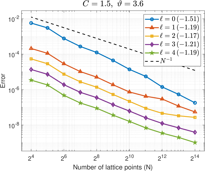
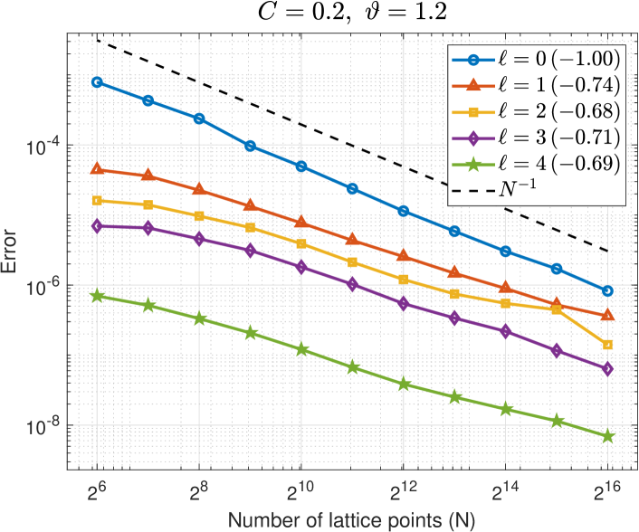
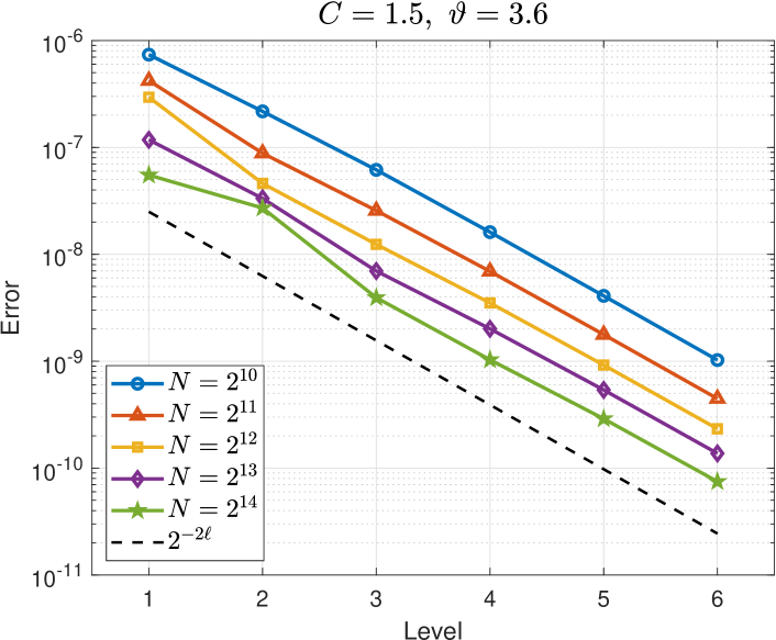
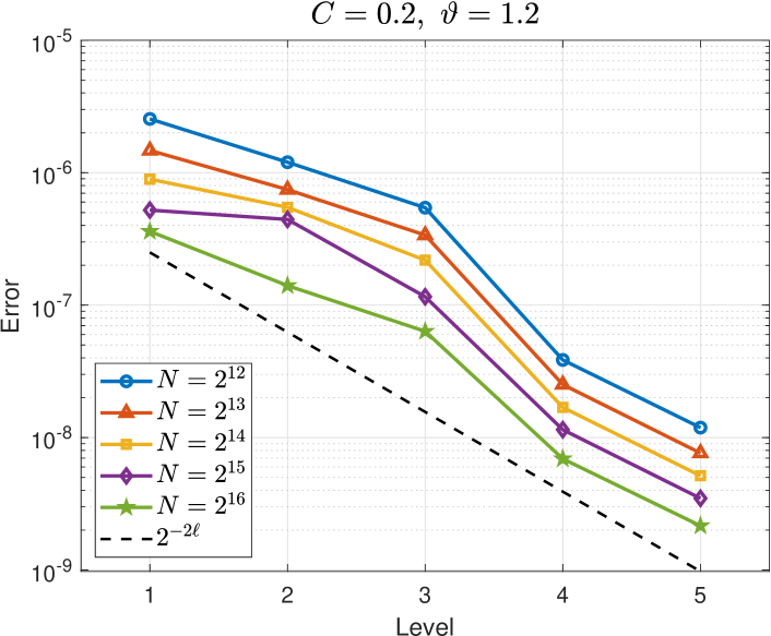
The top two plots in Figure 4 show that decreases with increasing for each . The case is exactly the single-level interpolation error , and we observe a faster rate of convergence compared to the interpolation error of the FE differences for . For the easier problem on the left, we observe for and on average for the other . For the harder problem on the right, we observe for and on average for the other . (The rates for are different to those observed in Figure 3 because we have here while in Figure 3.) These observed rates correspond to the value of in Assumption (M(M2)) of Theorem 6.
The bottom plots in Figure 4 show that decreases with increasing level for a range of values of . (Larger values of are used for the harder problem on the right.) This illustrates how the FE error changes on each level. We observe an error reduction of roughly , thus verifying that in Assumption (M(M2)) of Theorem 6.
7.3 Multilevel results
Figure 5 plots the computational cost, measured by CPU time in seconds, of the single-level and multilevel approximations against their respective errors for the two parameter sets. The errors are estimated by
where denotes either a single-level or multilevel approximation of , with , , , and is the maximum number of lattice points used to construct the approximation (i.e., for a multilevel approximation).
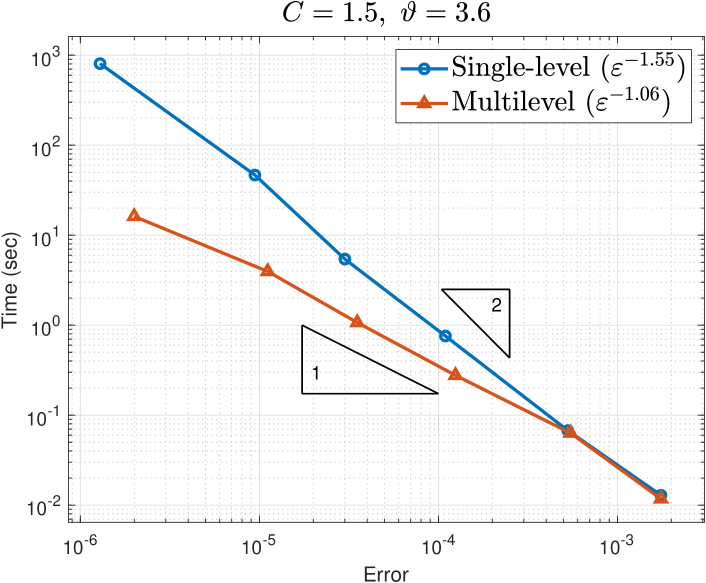
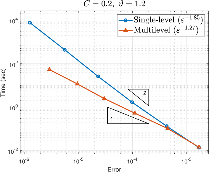
Starting from bottom right to top left within the plots in Figure 5, each data point of the single-level result corresponds to a decreasing FE mesh width with corresponding increasing number of lattice points from Table 1, while each data point of the multilevel result corresponds to an increasing total number of levels with the corresponding choices for taken from Table 1. The data point for the multilevel error coincides with the single-level error as expected.
Recall from (7.1) that the theoretical costs for the single-level and multilevel approximations to achieve an error are and , respectively. The triangles in the plots show gradients 1 and 2 as denoted. The observed costs shown in the legends of Figure 5 are mostly lower (better) than the theoretical costs. It may be that the theoretical rate of convergence used in estimating the cost in (7.1) is overly pessimistic. We can instead estimate the cost using the observed rates for from Figure 4.
For the easier problem on the left of Figure 4, we observe and (average) for single-level and multilevel errors, respectively, giving the expected costs and , respectively. These are closer to the corresponding observed costs and on the left of Figure 5.
For the harder problem on the right of Figure 4, we observe and (average) for single-level and multilevel errors, respectively, giving the expected costs and , respectively. These again are closer to the corresponding observed costs and on the right of Figure 5.
These observations have been replicated for several other parameter sets, which are omitted for brevity.
8 Conclusion
This paper introduces a multilevel kernel method for approximating solutions to PDEs with periodic coefficients over the parametric domain. A theoretical framework is developed with full detail, including error estimates for the multilevel method and a comprehensive cost comparison between the single-level and multilevel approaches. The construction of the multilevel approximation is also outlined and is supported by numerical experiments demonstrating the advantages of the multilevel approximation for different choices of parameters with varying levels of difficulty.
When applying multilevel methods to integration, randomisation can be used to compute an unbiased mean-square error estimate, and the number of levels and/or samples per level can be adaptively adjusted on the run. In contrast, a practical challenge in applying the multilevel kernel approximation is that there is no efficient adaptive multilevel approximation strategy. This is because the error cannot be effectively evaluated during the implementation, since any estimation must be done with respect to some reference solution. This requires either solving the PDE again at several sample points or constructing an expensive single-level proxy of the true solution, defeating the purpose of applying multilevel approximation. We leave investigations into adaptive multilevel kernel approximation for future research.
References
- [1] G. Byrenheid, L. Kämmerer, T. Ullrich and T. Volkmer, Tight error bounds for rank-1 lattice sampling in spaces of hybrid mixed smoothness, Numer. Math. 136 993–1034, (2017).
- [2] J. Charrier, R. Scheichl and A. L. Teckentrup, Finite element error analysis of elliptic PDEs with random coefficients and its application to multilevel Monte Carlo methods, SIAM J. Numer. Anal. 51, 332–352 (2013).
- [3] P. G. Ciarlet, The Finite Element Method for Elliptic Problems SIAM, Philadelphia, PA, USA, 2002.
- [4] K. A. Cliffe, I. G. Graham, R. Scheichl and L. Stals, Parallel computation of flow in heterogeneous media using mixed finite elements, J. Comput. Phys. 164, 258–282 (2000).
- [5] K. A. Cliffe, M. B. Giles, R. Scheichl and A. L. Teckentrup, Multilevel Monte Carlo methods and applications to elliptic PDEs with random coefficients, Comput. Visual. Sc. 14, 3–15 (2011).
- [6] A Cohen, R. De Vore and Ch. Schwab, Convergence rates of best N-term Galerkin approximations for a class of elliptic sPDEs, Found. Comput. Math. 10, 615–646 (2010).
- [7] R. Cools, F. Y. Kuo, D. Nuyens and I. H. Sloan, Lattice algorithms for multivariate approximation in periodic spaces with general weight parameters, Contemp. Math. 754, 93–113 (2020)
- [8] R. Cools, F. Y. Kuo, D. Nuyens and I. H. Sloan, Fast component-by-component construction of lattice algorithms for multivariate approximation with POD and SPOD weights, Math. Comp. 90, 787–812 (2021).
- [9] M. Croci and P. E. Farrell, Complexity bounds on supermesh construction for quasi-uniform meshes, J. Comput. Phys. 414, 1–7 (2020).
- [10] M. Croci, M. B. Giles , M. E. Rognes and P. E. Farrell, Efficient white noise sampling and coupling for multilevel Monte Carlo with nonnested meshes, SIAM/ASA J. Uncertain. Quantif. 6, 1630–1655 (2018).
- [11] N. Dyn, Interpolation and approximation by radial and related functions, In: Approximation Theory VI (C. Chui, L. Schumaker, and J. Ward, eds), Academic Press (New York), 211–223 (1989).
- [12] P. E. Farrell, M. D. Piggott, C. C. Pain, G. J. Gorman and C. R. Wilson, Conservative interpolation between unstructured meshes via supermesh construction, Comput. Methods Appl. Mech. Engrg. 198, 2632–2642 (2009)
- [13] A. D. Gilbert and R. Scheichl, Multilevel quasi-Monte Carlo for random elliptic eigenvalue problems I: regularity and error analysis, IMA J. Numer. Anal. 44, 466–503 (2024).
- [14] A. D. Gilbert, F. Y. Kuo and A. Srikumar, Density estimation for elliptic PDE with random input by preintegration and quasi-Monte Carlo methods, to appear in: SIAM J. Numer. Anal., arXiv:2402.11807 (2025).
- [15] M. B. Giles, Improved multilevel Monte Carlo convergence using the Milstein scheme, In: Monte Carlo and Quasi-Monte Carlo Methods 2006 (A. Keller, S. Heinrich, and H. Niederreiter, eds), Springer-Verlag, 343–358 (2007)
- [16] M. B. Giles, Multilevel Monte Carlo path simulation, Oper. Res. 56, 607–617 (2008).
- [17] M. B. Giles, Multilevel Monte Carlo methods, Acta Numer. 24, 259–328 (2015).
- [18] M. B. Giles and B. J. Waterhouse, Multilevel quasi-Monte Carlo path simulation, Radon Series Comp. Appl. Math., 8, 1–18 (2009)
- [19] I. G. Graham, F. Y. Kuo, J. A. Nichols, R. Scheichl, Ch. Schwab and I. H. Sloan, Quasi-Monte Carlo finite element methods for elliptic PDEs with lognormal random coefficients, Numer. Math., 131, 329–368 (2015).
- [20] H. Hakula, H. Harbrecht, V. Kaarnioja, F. Y. Kuo and I. H. Sloan, Uncertainty quantification for random domains using periodic random variables, Numer. Math. 156, 273–317 (2024)
- [21] R. L. Hardy Multiquadric equations of topography and other irregular surfaces, J. Geophys. Res. 76, 1905–1915. (1971).
- [22] S. Heinrich, Multilevel Monte Carlo methods, Lecture notes in Compu. Sci. Vol. 2179, 3624–3651, Springer (2001)
- [23] V. Kaarnioja, Y. Kazashi, F. Y. Kuo, F. Nobile and I. H. Sloan, Fast approximation by periodic kernel-based lattice-point interpolation with application in uncertainty quantification, Numer. Math. 150, 33–77 (2022).
- [24] V. Kaarnioja, F. Y. Kuo and I. H. Sloan, Uncertainty quantification using periodic random variables, SIAM J. Numer. Anal. 58, 1068–1091 (2020).
- [25] V. Kaarnioja, F. Y. Kuo and I. H. Sloan, Lattice-based kernel approximation and serendipitous weights for parametric PDEs in very high dimensions, In: Monte Carlo and Quasi-Monte Carlo Methods 2022 (A. Hinrichs, P. Kritzer and F. Pillichshammer, eds.), Springer-Verlag, 81–103 (2024)
- [26] L. Kämmerer, Reconstructing hyperbolic cross trigonometric polynomials from sampling along rank-1 lattices, SIAM J. Numer. Anal., 51, 2773–2796 (2013).
- [27] L. Kämmerer, Multiple rank-1 lattices as sampling schemes for multivariate trigonometric polynomials, J. Fourier. Anal. Appl., 24, 17–44 (2018).
- [28] L. Kämmerer, D. Potts and T. Volkmer, Approximation of multivariate periodic functions by trigonometric polynomials based on rank-1 lattice sampling, J. Complexity, 31, 543–576 (2015).
- [29] F. Y. Kuo, G. Migliorati, F. Nobile and D. Nuyens, Function integration, reconstruction and approximation using rank-1 lattices Math. Comp., 90, 1861 – 1897 (2021).
- [30] F. Y. Kuo, W. Mo and D. Nuyens, Constructing embedded lattice-based algorithms for multivariate function approximation with a composite number of points, Constr. Approx., 61, 81–113 (2025).
- [31] F. Y. Kuo, W. Mo, D. Nuyens, I. H. Sloan and A. Srikumar, Comparison of two search criteria for lattice-based kernel approximation, In: Monte Carlo and Quasi-Monte Carlo Methods 2022 (A. Hinrichs, P. Kritzer and F. Pillichshammer, eds), Springer Verlag, 413–429 (2024)
- [32] F. Y. Kuo and D. Nuyens, Application of quasi-Monte Carlo methods to elliptic PDEs with random diffusion coefficients – a survey of analysis and implementation, Found. Comput. Math. 16, 1631–1696 (2016).
- [33] F. Y. Kuo, Ch. Schwab and I. H. Sloan, Quasi-Monte Carlo finite element methods for a class of elliptic partial differential equations with random coefficients, SIAM J. Numer. Anal. 50, 3351–3374 (2012).
- [34] F. Y. Kuo, Ch. Schwab and I. H. Sloan, Multilevel quasi-Monte Carlo finite element methods for a class of elliptic partial differential equations with random coefficients, Found. Comput. Math. 15, 411–449 (2015).
- [35] F. Y. Kuo, I. H. Sloan and H. Wózniakowski, Lattice rules for multivariate approximation in the worst case setting, In: Monte Carlo and Quasi-Monte Carlo Methods 2004 (H. Niederreiter and D. Talay, eds), Springer Verlag, 289–330, (2006).
- [36] F. Y. Kuo, I. H. Sloan and H. Wózniakowski, Lattice rule algorithms for multivariate approximation in the average case setting, J. Complexity. 24, 283–323, (2008).
- [37] F. J. Narcowich, J. D. Ward and H. Wendland, Refined error estimates for radial basis function interpolation, Constr. Approx. 19, 541–564, (2003).
- [38] PVC (Research Infrastructure), UNSW Sydney, Katana. (2010) doi:10.26190/669X-A286
- [39] J. Quaintance and H. W. Gould, Combinatorial Identities for Stirling Numbers: The Unpublished Notes of H. W. Gould, World Scientific Publishing Company, River Edge, NJ, (2015).
- [40] R. Schaback and H. Wendland, Kernel techniques: from machine learning to meshless methods, Acta Numer. 15, 543–639 (2006).
- [41] I. H. Sloan and V. Kaarnioja, Doubling the rate: improved error bounds for orthogonal projection with application to interpolation, BIT Numer. Math. 65 (Online) (2025)
- [42] I. H. Sloan and H. Woźniakowski, Tractability of multivariate integration for weighted Korobov classes, J. Comp. 17, 697–721 (2001).
- [43] A. L. Teckentrup, P. Jantsch, C. G. Webster and M. Gunzburger, A multilevel stochastic collocation method for partial differential equations with random input data, SIAM-ASA J. Uncert. Quantif. 3, 1046–1074 (2015).
- [44] A. L. Teckentrup, R. Scheichl, M. B. Giles and E. Ullmann, Further analysis of multilevel Monte Carlo methods for elliptic PDEs with random coefficients, Numer. Math. 125, 569–600 (2013).
- [45] H. Wendland, Scattered Data Approximation, Cambridge University Press, Cambridge (2005)
- [46] Z. M. Wu and R. Schaback, Local error estimates for radial basis function interpolation of scattered data, IMA J. Numer. Anal. 13, 13–27 (1993).
- [47] Z. Y. Zeng, P. Kritzer and F. J. Hickernell, Spline methods using integration lattices and digital nets, Constr. Approx. 30, 529–555 (2009).
- [48] Z. Y. Zeng, K. T. Leung and F. J. Hickernell, Error analysis of splines for periodic problems using lattice designs, In: Monte Carlo and Quasi-Monte Carlo Methods 2004 (H. Niederreiter and D. Talay, eds) Springer Verlag, 501–514 (2006)
Appendix I Combinatorial identities and proofs
This appendix provides some important combinatorial results that are required in the proofs of several regularity theorems. First, we provide an identity to simplify sums involving Stirling numbers of the second kind (2.1) from [39],
| (I.1) |
Lemma 11.
Let and let , and be sequences of non-negative real numbers that satisfy the recurrence
| (I.2) |
where is the multi-index whose the th component is 1 and all other components are 0. Then
| (I.3) |
where for are Stirling numbers of the second kind given by (2.1). The result also holds with both equalities replaced by inequalities .
Proof.
The statement is proved by using induction on . The statement holds trivially for since . Assume the statement (I.3) holds for all multi-indices of order less than , i.e., if for some , then
| (I.4) |
We now prove the statement for indices of order . Substituting the induction hypothesis (I.4) into (I.2), we have
| (I.5) |
where
We use a dash to denote multi-indices with the th component removed, for example, and adopt the notation . Then
| (I.6) |
where we have rearranged the terms and swapped the order of the sums.
Recognising that
we have
| (I.7) |
where we get to the second line by relabelling the summation indices of the second sum from to and to the third line by swapping the order of sums indexed by and . Swapping the order of the summations indexed by and in gives
| (I.8) |
where the second equality is obtained using (I.1) and the third equality is from a simple re-indexing of the sum. To reach the final line, we can add the terms corresponding to into the sum so that the sum begins from because these terms are all equal to 0 due to the presence of an factor in the terms of the series, provided that we also introduce the condition to ensure the factorial term is defined. Substituting (I.8) into (I.7) gives
where we have added the terms corresponding to into the summation over since these terms are all also equal to 0 as when . Substituting this formula for back into (I) then rearranging gives
where we obtain the last line by combining the sums over and into a single sum over the original index and combine the sums over and into a single sum over the index .
Now substituting this back into (I.5), we have
which is our desired result. We move to the second line interchanging the order of the summations and then to the third line by including the case when and subtracting the corresponding term to maintain equality. Since when , the term only contributes when , and the resulting sum cancels out with the term giving the required result.
From [20, Lemma A.3], we also have that for some ,
| (I.9) |
where and are arbitrary sequences of real numbers.
Appendix II Parametric regularity proofs
-
Proof of Lemma 2.
We follow a similar strategy to the proof of [32, Lemma 6.2]. For , we rewrite the strong formulation (1.1) using the product rule to obtain
from which it follows that
where we have used Assumption (A(A0)) and the definition . Combining this with (2.4), we have
where
(II.1) and is the Poincaré constant of the embedding . It follows from Assumption (A(A0)) that is finite. Hence, and (4.1) holds for .
Recall that the gradient and Laplacian are taken with respect to and that is taken with respect to . For , we take the th derivative of (1.1) using the Leibniz product rule. Since is independent of , the right-hand side is 0 and we can rearrange the resulting expression to obtain, omitting the dependence of and ,
(II.2) where we use the fact that the mixed partial derivatives of with respect to are
(II.3) Expanding (Proof of Lemma 2.) using the product rule for and rearranging gives
Now taking the norm and applying the triangle inequality gives
where we used for all real . Formulating the above into a recursion gives
(II.4) where and are defined in (2.3) and we define
Substituting (2.5) into , we can bound by
(II.5) We simplify using the same strategy in the proof of Lemma 11 by separating out the th component of the sum over and interchanging the order of the sums to give
where we drop the condition since if and , there exists some index such that and . We have also replaced with since for all .
Substituting the bound on into (Proof of Lemma 2.) and using , we can bound by
where is defined in (II.1). Thus, defining , we can write (II.4) as
Noting that , we can then apply Lemma 11 (we cannot apply Lemma 11 to (II.4) with since it is not true that ) to give
Then, using (I) and the identity from [32], we obtain,
as required.
-
Proof of Lemma 3.
We follow the proof strategy presented in [32, Lemma 6.3]. Let , and . Since is analytic in , we have that for every and hence
where is the orthogonal projection defined by (2.11). It then follows that
(II.6) where we have omitted the dependence of on and for brevity.
Starting with the Galerkin orthogonality property given in (2.10), we take the derivative with respect to using the Leibniz product rule to give
(II.7) Next, separating out the term when and then substituting the mixed derivatives of the coefficient (II.3) into (II.7), we obtain
for all . Now, letting , we have
(II.8) Since , using (2.11) with and yields
which can then be rearranged to give
(II.9) where we have used Assumption (A(A0)). Substituting in the lower bound (II.9) for the left-hand side of (Proof of Lemma 3.), applying the Cauchy-Schwarz inequality to the right hand side and then dividing through by yields
Then substituting this into (Proof of Lemma 3.) gives
where is defined in (2.3).
Applying Lemma 11 with , and to the above inequality gives
Since , we have from (2.12) (with independent of ), which in turn gives
Then using (4.1) from Lemma 2 with constant , and defining , we obtain
We arrive at the first equality using (I) with and and then move to the last line using the identity from [32]
which gives the required result. The constant is independent of and .
-
Proof of Lemma 4.
We use an Aubin-Nitsche duality argument. For some linear functional , define to be the solution to the dual problem,
which, since is symmetric, is equivalent to the parametric variational problem (2.2) with replaced by , the representer of . Thus, inherits the regularity of the solution to (2.2) and the FE approximation also satisfies (4.2).
Letting (and suppressing the dependence on ), it follows from Galerkin orthogonality(2.10) that , which leads to
Differentiating this with respect to gives
Applying the Leibniz product rule, the integrand on the right becomes
where we have substituted in the bound (II.3) and applied the Leibniz product rule to .
Now, taking the absolute value and using the Cauchy-Schwarz inequality gives
| (II.10) | ||||
where we have also used the definition of in (2.3).
The terms in the first sum in (II.10) can be bounded by (4.2) from Lemma 3 to give
| (II.11) |
where denotes the constant factor from (4.2) and we obtain the last equality using (I) with and , along with the identity from [32]
| (II.12) |
Similarly, for the summation over the index in (II.10), we again use (4.2) from Lemma 3 along with (I) and (II.12) to obtain
Substituting this back into the sum indexed by in (II.10), we have
| (II.13) |
To bound , we use the same technique as in Lemma 11. We separate out component from the innermost sum over , bound by then swap the order of the sums over and so that (I.1) can be used to evaluate the sum over . This gives
We can add the terms to the sum due to the presence of the factor and thus
and using we have,
| (II.14) |
Finally, we let be the functional with representer , i.e., for , which gives
where the implied constant is independent of and .
Finally, dividing through by
yields the required result (4.2).