Multilevel Preconditioner with Stable Coarse Grid Corrections for the Helmholtz Equation
Abstract
In this paper we consider a class of robust multilevel precontioners for the Helmholtz equation with high wave number. The key idea in this work is to use the continuous interior penalty finite element methods (CIP-FEM) studied in [19, 21] to construct the stable coarse grid correction problems. The multilevel methods, based on GMRES smoothing on coarse grids, are then served as a preconditioner in the outer GMRES iteration. In the one dimensional case, convergence property of the modified multilevel methods is analyzed by the local Fourier analysis. From our numerical results, we find that the proposed methods are efficient for a reasonable range of frequencies. The performance of the algorithms depends relatively mildly on wave number. In particular, only one GMRES smoothing step may guarantee the optimal convergence of our multilevel algorithm, which remedies the shortcoming of the multilevel algorithm in [5].
Keywords. Multilevel method, Helmholtz equation, high wave number, continuous penalty finite element method, GMRES method, local Fourier analysis
1 Introduction
The efficient and accurate numerical approximation of high frequency wave propagation is of fundamental importance in many applications such as acoustic, electromagnetic, elasticity and geophysical surveys. When the problem is linear and time-harmonic, it can be typically modeled by Helmholtz equation. The interest of this paper is to consider the Helmholtz equation with Robin boundary condition which is the first order approximation of the radiation condition:
| (1.1) | ||||
| (1.2) |
where is a polygonal/polyhedral domain, is known as the wave number, denotes the imaginary unit, and denotes the unit outward normal to .
For high wave number , the linear system from the discretization of Helmholtz equation is usually strongly indefinite, causing most of iterative methods to converge slowly or diverge. In recent years, there have been many advances in the development of iterative methods and preconditioners for the solution of the Helmholtz equation (cf. [10, 11]).
Due to high efficiency of multilevel methods for positive definite problems, more and more attentions have been received to develop robust multilevel methods for Helmholtz equation. However, a direct application of multilevel methods with standard smoothing and coarse grid correction are ineffective. Some strategies have been proposed to remedy the problem (cf. [3, 5, 15, 16]). For instance, Elman, Ernst and O’Leary [5] proposed GMRES smoothing together with flexible GMRES acceleration. But in order to achieve convergence, a relatively large number of GMRES smoothing steps are needed on the intermediate grids. Another approach, the so-called wave-ray multigrid methods [3, 16], was proposed by Brandt and Livshits through defining a meaningful coarse problem by augmenting the standard V-cycle with ray grids and using coarse grid basis derived from plane waves. This method performs well with increasing wave number, but it does not easily generalize to unstructured grids and complicated Helmholtz problems. Alternatively, instead of applying multigrid iterations directly to the Helmholtz equation, a class of shifted Laplacian preconditioners [8, 9] has recently attracted a lot of attention, which precondition the Helmholtz equation with a complex shifted operator and is shown to be an efficient Krylov method preconditioner. We would like to mention that Engquist and Ying [6, 7] recently proposed two new types of sweeping preconditioners for central difference scheme of the Helmholtz equation based on an approximate factorization by sweeping the domain layer by layer starting from an absorbing layer. Similar to the wave-ray multigrid methods, the new preconditioners have a nearly linear computational cost and the number of outer iterations is essentially independent of the number of unknowns and the wave number when combined with the GMRES solver.
Our objective is to develop robust multilevel methods for the Helmholtz problem (1.1)-(1.2). Although the pollution error is inherent in the standard finite element methods (FEM) to solve Helmholtz equation, the FEM can still be used on fine grid whose mesh size is sufficiently small to reduce the pollution error. In a recent work [21], the pre-asymptotic analyses of both the FEM and the continuous interior penalty finite element methods (CIP-FEM) are given. In particular, the well-posedness of standard FEM has been proved under the condition of , where is mesh size, is the polynomial order of approximation space, and is a constant independent of . Thus, without this condition, the well-posedness of standard FEM on coarse grids in the multilevel method can not be guaranteed. Moreover, oscillations on the scale of the wavelength can not be resolved well by standard FEM on the coarse grids. By contrast, the CIP-FEM has been proved in [21] that the associated discrete problem is always well-posed without any mesh condition. Intrinsically, the main technique in the stable CIP-FEM is to add a complex shift in the bilinear form, which is similar to the idea of shifted Laplace preconditioner approach. Comparing to adding a shift to the original problem in shifted Laplace operator, the well-posed CIP-FEM is consistent with the original equation and only changes the discrete bilinear form. Based on these observations, the new approach proposed in this work is to apply the CIP-FEM to construct the stable coarse grid correction problems. Standard Jacobi or Gauss-Seidel smoothers become unstable on the coarse grids, especially on the intermediate grids in multilevel methods. Motivated by the smoothing approach presented in [5], the smoothing in this work is to use GMRES method based on CIP-FEM on the coarse grids, and standard Jacobi or Gauss-Seidel relaxation on the fine enough grids. From our numerical experiments, we find that the number of GMRES smoothing steps in our algorithm can be much smaller than that in [5], even if one GMRES smoothing step may guarantee the optimal convergence of our multilevel algorithm.
Our main tool to analyze the multilevel methods for Helmholtz equation is the Local Fourier analysis (LFA), which has been introduced for multigrid analysis by Achi Brandt in 1977 [2]. Comprehensive surveys can be found in [18] and the references therein. We mainly utilize the LFA to analyze smoothing properties of relaxations and convergence properties of two- and three-level methods in one dimensional case. This may provide quantitative insights into the multilevel methods for Helmholtz problem (1.1)-(1.2).
The remaining part of this paper is organized as follows: In section 2, we introduce some notation, recall the formulation of CIP-FEM, and present the multilevel method for the linear system from CIP-FEM approximation. Section 3 is to present the modified multilevel method for Helmholtz problem. Standard FEM is used on fine enough grids, on coarse grids the CIP-FEM is utilized instead. Section 4 is devoted to the LFA of the multilevel method for one dimensional Helmholtz problem, we focus on the smoothing analysis and two- and three-level analysis. In the last section, we give some numerical results to illustrate the performance of the proposed multilevel methods.
2 Notations and Preliminaries
2.1 Formulation of CIP-FEM
Let be a conforming quasi-uniform triangulation of , and denote the collection of edges/faces by , while the set of interior edges/faces by and the set of boundary edges/faces by . For any , we define . Similarly, for , define . Let . Throughout this paper we use the standard notations and definitions for Sobolev spaces (cf. [1]). In particular, and for denote the -inner product on complex-valued and spaces, respectively. Denote by and .
Now we define the energy space . For any and an interior edge/face , where and are two distinct elements of with respective outer normals and , we introduce the jump . Define the sesquilinear form on as follows:
where
| (2.1) |
where is a complex number with positive imaginary part. The terms in are so-called penalty terms and are penalty parameters (cf. [19, 21]).
We define the CIP approximation space as the standard finite element space of order , i.e.,
where is the space of polynomials of degree at most on . The CIP finite element approximation is to find such that
| (2.3) |
It is clear that if the parameters , then the CIP-FEM reduces to the standard FEM. It has been proved that the CIP-FEM is stable for any [19, 21]. The penalty parameters may be tuned to reduce the pollution errors. The numerical results in [19] show that using about the same total degrees of freedom (DOFs), the CIP-FEM yields the least phase error comparing to the standard FEM and IPDG method [12].
2.2 Multilevel methods for CIP-FEM
Let be a shape regular family of nested geometrically conforming simplicial triangulations of the computational domain obtained by successive quasi-uniform refinement of an intentionally chosen coarse grid . We denote by the CIP approximation space on . It is easy to see that the spaces are nested, i.e., . But the bilinear forms defined as in (2.3) on each are nonnested. Thus in this work we consider the following multilevel methods for CIP-FEM discretizations, which has also been used for solving the linear systems from nonconforming P1 finite element approximations (cf. [17]).
For brevity, we denote by the bilinear form on , where is the mesh size of . Define projections , : according to
The existence and uniqueness of the discrete problem (2.3) imply the well-posedness of each . For , we also define by means of
| (2.4) |
Define by
Then the CIP-FEM on level (cf. (2.3)) can be rewritten as:
| (2.5) |
For the smoothing strategy, in fact, when is small enough, either of weighted Jacobi and Gauss-Seidel relaxation can be applied. Otherwise, GMRES relaxation can be used as a smoother and this will be explained in the following sections. To be precise, we describe the smoothing strategy as follows:
Definition 2.1.
Let . Given and , let and . If , let be the weighted Jacobi relaxation or Gauss-Seidel relaxation based on . Otherwise, when we use the GMRES relaxation based on .
We remark that we choose in this paper. This choice is motivated by the efficient relaxation of Jacobi and Gauss-Seidel smoothers, and it ensures that the amplification factor for the Jacobi and Gauss-Seidel smoothers will not become too large (cf. section 4.3 in the following and section 2.1 in [5]). When , we also define the operator by
| (2.6) |
We can now state the multilevel method for solving the CIP-FEM discretization system on level which is non-recursive version of multilevel method.
Algorithm 2.1.
Given an arbitrarily chosen initial iterate , we seek as follows:
Let .
-
For . When or ,
Otherwise, perform GMRES relaxation for the correction problem and set . Here is a scaling parameter to weaken the influence of the error during prolongations. In this paper, we always set .
-
For . When or ,
Otherwise, perform GMRES relaxation based on as in step 1 to get .
-
Set .
Here we note that the GMRES relaxation is not linear in the starting value, and the error operator of the above algorithm can not be written directly in a product form which holds only for the particular case . When this particular case is considered reasonably, we set
Then the error operator of Algorithm 2.1 for the case can be derived as
| (2.7) |
where is the identity operator in .
3 Modified multilevel methods for standard FEM
In general, in order to reduce the pollution error, 6-10 grid points per wavelength are typically chosen to yield reasonable accuracy. In a unit square domain , it is well know that , where is the number of points per wavelength (cf. [14]), implies the deterioration of for increasing grid points per wavelength. In theory, the well-posedness of discrete solution by CIP-FEM holds for any and , but it is not guaranteed for discrete solution by standard FEM on coarser grids with particularly [19, 21], where the constant is independent of and . Therefore, in order to establish stable coarse grid correction problems in multilevel methods for Helmholtz equation, the CIP-FEM will be applied on the coarse grids. Besides, for standard FEM, eigenvalues of discrete system close to the origin may undergo a sign change after discretization on a coarser grid. If a sign change occurs, the coarse grid correction does not give a convergence acceleration to the finer grid problem but gives a severe convergence degradation instead. This is analyzed in [5] and a remedy combining GMRES method as a smoother on coarse grids is proposed. This idea has been applied in Algorithm 2.1, and we will also utilize this strategy in the following modified multilevel methods to get more efficient smoother for indefinite discrete systems.
For brevity, let denote the linear operator with the parameters , i.e., the linear operator for standard FEM, and energy operator . The discrete problem on level is for CIP-FEM (cf. (2.5)) or for standard FEM. When the mesh size is sufficiently small to reduce the pollution error and satisfy the accuracy requirement, both CIP-FEM and standard FEM can be utilized. However, the nonzero elements of linear system from standard FEM may be less than that from CIP-FEM, and when the grid is fine enough, the pollution error by the standard FEM is also small. Thus, we may still apply the standard FEM on the fine grids.
Similar to Definition 2.1, we use the smoothing strategy on each as follows.
Definition 3.1.
Let . Given and . If , let be the weighted Jacobi relaxation or Gauss-Seidel relaxation based on . Otherwise, when we use the GMRES relaxation based on .
When , the operator is defined similarly as in (2.6). Now we state the modified multilevel method for the discrete system from standard FEM for the Helmholtz problem (1.1)-(1.2) as follows.
Algorithm 3.1.
Given an arbitrarily chosen initial iterate and integers , we seek as follows:
Let .
-
For . Given is chosen as in Algorithm 2.1, when or ,
where if , if . Otherwise, perform steps of GMRES relaxation for the correction problem and set .
-
For . When or ,
where if , if . Otherwise, perform steps of GMRES relaxation for the correction problem and set .
-
Set .
Remark 3.1.
In [5], in order to prevent unnecessary damping of smoothing modes which should be handled by the coarse grid correction, the postsmoothing is always favored over presmoothing (cf. section 3.2 in [5]). This is also true in our work. However, due to the utilization of stable coarse grid correction method, the above algorithm will converge even when the smoothing is chosen as one step in both post- and presmoothing.
Remark 3.2.
Comparing to Algorithm 2.1, the CIP-FEM is only applied in the coarse grid correction when in the above algorithm. From the first numerical example in this paper, we can see that the convergence property of this two algorithms is similar. Actually, this phenomena can also be observed in the following LFA. In order to reduce computations, one may prefer Algorithm 3.1 in practice.
4 The one dimensional local Fourier analysis
In this section, we aim to analyze different approaches based on Algorithm 2.1 for the discrete system from one dimensional Helmholtz equation, where standard FEM is utilized on the finest grid. We focus on the analysis for the discretization from linear continuous interior penalty finite element method (CIP-P1) by the important tool LFA in multigrid analysis. Here we mainly focus on the analysis of two-level methods. The LFA of three-level methods is also mentioned. The analysis will imply the efficiency of Algorithm 3.1. The following presentation is related to the notation and philosophy from [18].
4.1 Basic tools in one dimensional local Fourier analysis
The LFA is based on certain idealized assumptions and simplifications: the boundary conditions are neglected and the problem is considered on regular indefinite grids . Although the Robin boundary condition (1.2) and other absorbing boundary conditions are often applied in realistic Helmholtz problem, the neglect of boundary condition does usually not affect the validity of LFA (cf. [18]). The LFA in this section can be considered as simplification for the analysis of multilevel method for Helmholtz problem (1.1-1.2) in one dimension.
Let be a discrete operator with a stencil representation . For any defined on and a fixed point , reads in stencil notation as
where is a certain finite index defining the so-called stencil. The basic quantities in the LFA are the Fourier modes with and Fourier frequency . In fact, the frequency can be restricted to the interval as a fact that . It is easy to see that the Fourier modes are all the formal eigenfunctions of :
| (4.1) |
where the eigenvalues of can be presented as , which is called the Fourier symbol of the operator . Given a so-called low frequency , its complementary frequency is defined as
| (4.2) |
Interpreting the Fourier modes as coarse grid functions yields
The Fourier modes and are called -harmonics. These Fourier modes coincide on the coarse grid with mesh size , and they can be represented by a single coarse grid mode . Hence, each low frequency mode is associated with a high frequency mode. For a given , define the two dimensional subspace of -harmonics by
| (4.3) |
where is defined as in (4.2). A crucial observation is that the space is invariant under both smoothing operators and correction schemes for general cases by two-level method. The invariance property holds for many well-known smoothing methods (cf. [18]), such as Jacobi relaxation, lexicographical Gauss-Seidel relaxation, et al.
Let be a discrete two-level operator. In the following, we will show that a block-diagonal representation for consists of blocks (cf. [18]), which denotes the representation of on . Then the convergence factor of by the LFA is defined as follows:
where is the spectral radius of the matrix . We can refer to [18] for generalizations to -level analysis.
4.2 One dimensional Fourier symbols
Now we give the Fourier symbols of different operators in multilevel method for CIP-P1 discretization of one dimensional Helmholtz equation (1.1). We always assume for some constant in (2.1). Denote by , , . Since the boundary condition is neglected in the LFA, the stencil presentation of discretization operator from (2.4) can be derived as (cf. [20])
Combining the above expression and (4.1) yields the Fourier symbol of as
| (4.4) |
Obviously, the Fourier symbol of standard FEM with piecewise P1 approximation (FEM-P1) is .
For simplicity, we use standard weighted Jacobi (-JAC) and lexicographical Gauss-Seidel (GS-LEX) relaxations as the smoothers in the LFA. It is easy to derive the weighted Jacobi relaxation matrix as , where is indentity matrix, consists of the diagonal of and is a weighted parameter. Due to the fact that , one can easily deduce the Fourier symbol of weighted Jacobi relaxation as follows:
| (4.5) |
The GS-LEX relaxation matrix is , where is the strictly lower triangular part of and is the strictly upper triangular part of . The Fourier symbol of can also be directly derived that
| (4.6) |
Note that for the restriction matrix and , there holds
By an analogous stencil argument, the stencil presentation of full weighting restriction matrix can be derived to be . Then one can obtain the Fourier symbol of is
For the linear prolongation matrix , one can also derive its Fourier symbol as follows (cf. [18]):
4.3 Smoothing analysis
Weighted Jacobi and lexicographical Gauss-Seidel relaxations are the general smoothing operators. It is well-known that such two smoothers are unstable especially for linear systems from indefinite Helmholtz equation by standard FEM approximations. This is caused by negative eigenvalues of the associated linear system and divergence occurs under such two smoothers. To make up the problem, an improvement is introduced by the shifted Laplacian preconditioner [8, 9, 10], which preconditions the Helmholtz equation with a complex shifted operator
| (4.7) |
where are free parameter. The use of a shift is important to guarantee multilevel convergence, whereas the multilevel method for the shifted operator only converges for a sufficiently large shift. But this contradicts the fact that the outer Krylov acceleration prefers a small shift. Based on the idea of adding a shift to the original problem, we consider the stable CIP-FEM which is consistent with original equation and adds a complex shift in the bilinear form.
Recalling that every two dimensional subspace of -harmonics with is left invariant under the -JAC and GS-LEX relaxations, then the Fourier representation of smoother or with respect to can be written as
| (4.8) |
where is the smoother symbol derived in (4.5) and (4.6). The spectral radius of the smoother operator can be easily calculated since the above matrix is diagonal.
For simplicity, we concern on the weighted Jacobi relaxation. The frequency maximizing over can be calculated by its first and second derivatives, which reveal or maximizing . Hence, the spectral radius of can be deduced as follows: where
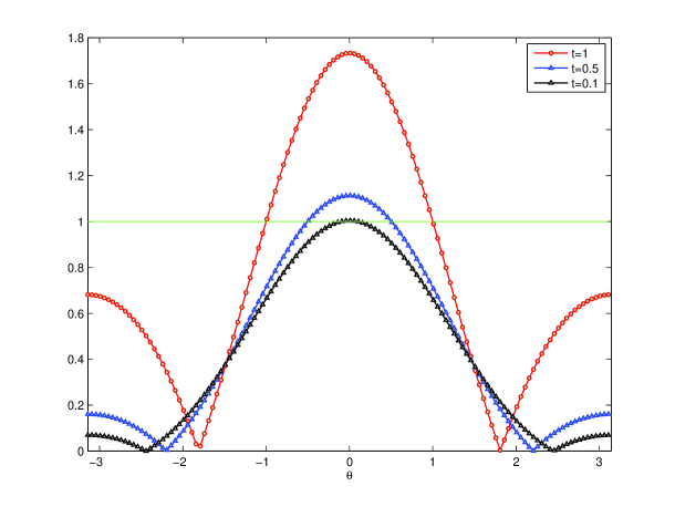
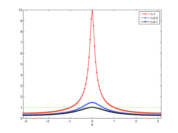
Since the parameter in CIP-FEM may influence the pollution error, it is critical to make a suitable choice. For the case , it has been derived in [20] that for one dimensional problem there exists an optimal choice such that the pollution error vanishes when the penalty parameter is chosen as , where the constant is independent of and . The left graph of Figure 1 shows the Fourier symbols for -JAC smoother with and . We find that always occur at the low frequencies, and small leads to a better relaxation. Similar phenomenon is observed for GS-LEX smoother in the right graph of Figure 1. Thus, for fixed wave number , both -JAC and GS-LEX relaxations can be used as smoother on fine grid. Actually, the relaxation properties of these two smoothers are similar when is a complex number.
When -JAC smoother is utilized in the standard P1 FEM approximation, then
| (4.9) |
Thus, for near , the error is amplified by the smoothing. For CIP-FEM, there is a (complex) shift in the bilinear form, therefore the amplification factor is reduced. This may permit the use of -JAC smoother again. In fact, in our modified multilevel method, GMRES iteration is used on the intermediate grids (cf. [5]). In contrast with -JAC and GS-LEX relaxations, the Fourier symbol can not be derived for GMRES smoothing. In the following, we will give some explanations for the performance of GMRES smoothing from the numerical approach.
For simplification, we consider the one dimensional Helmholtz equation on an interval with homogeneous Dirichlet boundary conditions. The piecewise P1 CIP-FEM discretization leads to a linear system with coefficient matrix (cf. [20])
| (4.17) |
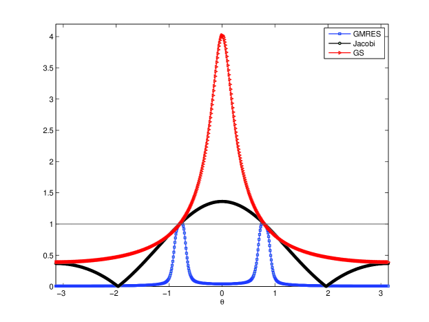
where . For , we apply the grid with mesh size , i.e., , and choose . Let the vector be an initial choice for smoothing, where , . We assume that is the relaxation iteration matrix and is the new vector after one step of smoothing. Then for fixed , we obtain the amplification factor for one step of smoothing , where stands for the Euclidean norm. Figure 2 shows the amplification factors of three different kinds of smoothing strategies: GS, Jacobi and GMRES relaxations. We can see that for high and low frequencies , the amplification factor of GMRES relaxation is always smaller than that of GS and Jacobi relaxations. The GMRES relaxation can still be convergent even when the other two smoothers lead to a divergent relaxation. The similar phenomenon can also be observed for other choices of and . Therefore, when standard Jacobi or GS relaxation fails as a smoother, we can replace this with the GMRES smoothing.
From the above analysis, we can see that for the relaxation of linear system for Helmholtz problem, the standard Jacobi or GS relaxation can be performed on the fine grids, but they fail on the coarse grids. In particular, the GMRES relaxation is efficient for smoothing on the intermediate coarse grids. In the next section, the correction scheme will be taken into account to obtain a more realistic convergence analysis of the multilevel method.
4.4 Two- and three-level local Fourier analysis
For more details about convergence property of multilevel method in Algorithm 3.1, we will focus on the LFA of two-level method. The LFA of three-level method will also be mentioned. For simplicity, we consider the case without postsmoothing. Since the Fourier symbol can not be obtained for GMRES smoothing, we only consider the two and three level methods with -JAC or GS-LEX relaxation. Then the iteration operator of Algorithm 3.1 in this case is the nonsymmetric version and can be derived as in (2.7). Three cases of iteration operator will be analyzed in the following: multilevel methods by shifted Laplace approach, multilevel methods with stable CIP-FEM coarse grid corrections, and multilevel methods with stable CIP-FEM for fine grid smoothing and coarse grid corrections.
The iteration operator of two-level method can be written as , and the operator is chosen for the corresponding algorithm. Since standard FEM is applied on the finest grid, we have , where is smoother determined by the algorithm. When CIP-FEM is used for smoothing on the grids and respectively, the iteration matrix is given by
Here, for , is smoothing relaxation matrix, with the same size as is identity matrix, is prolongation matrix from level to , is restriction matrix from level to , and stands for matrix representation of smoother with CIP-FEM approximation. Let (cf. [4]) stand for two-level iteration matrix, taking the smoothing based on shifted Laplace operator (4.7) with standard FEM approximation. Similarly, when applying standard FEM for smoothing on and CIP-FEM for correction on , the associated iteration matrix is derived as
where , and stands for smoothing matrix representation of with standard FEM approximation.
Since every two dimensional subspace (4.3) of -harmonics with is left invariant under -JAC or GS-LEX smoothing operator and correction operator, the representation of two-level iteration matrix of on is given by a matrix as follows:
| (4.31) | |||||
where is identity matrix and the subscript-D denotes the transformation of a vector into a diagonal matrix. Similarly, the representation of two-level iteration matrix based on shifted Laplace operator, can be easily obtained (cf. [4]). For the iteration operator , its representation on is given by
| (4.41) | |||||
Then the spectral radius of and for different can be obtained analytically and numerically.
The left graph of Figure 3 shows the spectral radius of with and over , and , under -JAC relaxation for on the finest grid. In order to make some comparisons between different algorithms, the penalty parameter in the CIP-FEM is always chosen as a complex number in the following if there is no special notation. If no confusion is possible, we will always denote for on the finest grid. The parameter in -JAC relaxation is always chosen as in this section. We observe that for most of the frequencies the spectral radius is smaller than one. The spectral radius tends to larger than one only under a few frequencies. Actually, the appearance of such a resonance is caused by the coarse grid correction and originates from the inversion of the coarse grid discretization symbol, in (4.31) and (4.41) for instance. The minimum of maximizes the spectral radius of and for fixed and .
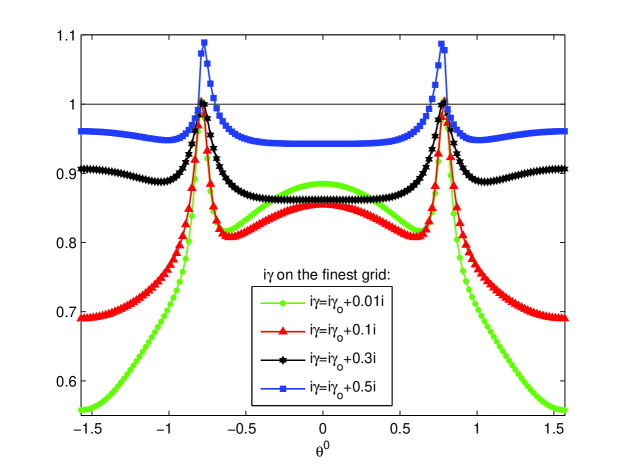
Moreover, for different choices of parameter in shifted Laplace operator, the properties of and with on the finest grid always perform better than that of . Although the spectral radius of with is almost equivalent to that of over the frequencies spreading near zero, there is a relatively large resonance causing by the coarse grid correction. Small in (4.7) deteriorates the coarse grid correction. However, large amplifies the corresponding spectral radius over the frequencies spreading near zero. We can refer to a recent work [4] about the choice of minimal complex shift parameter in shifted Laplace preconditioner. The choice of in or would also influence its spectral radius. The right graph of Figure 3 shows the spectral radius of with different under -JAC relaxation for . The influence of in is similar to in shifted Laplace preconditioner. For other small , the properties of , and can also be observed as above. Moreover, when on the finest grid is small enough, the spectral radiuses of , and can all be smaller than one over all . Due to the fact that our aim is to study the influences of smoothing corrections in two- and three-level methods, in the following we do not always assume to be sufficiently small.
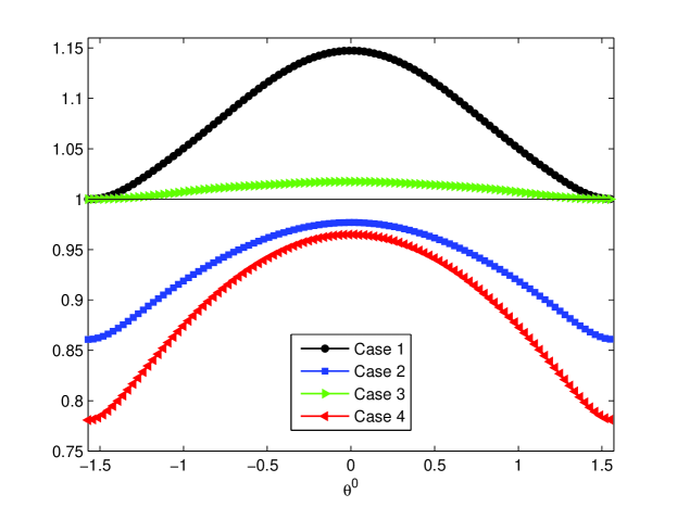
Alternatively, for large , the maximum of spectral radiuses of , and appear to be spread around . Actually, for large the main factor determining the spectral radius is the smoothing operator rather than the coarse grid correction. We assume that -JAC relaxation is used as smoother. It can be observed from Figure 4 that and reach a maximum in for and . Indeed, it has been analyzed in previous section and [4] that for CIP-FEM and shifted Laplace preconditioner (4.7) with continuous piecewise P1 approximation reaches a maximum at or . From (4.9), it is easy to see that the -JAC relaxation for discrete system from standard P1 FEM approximation is inefficient when is near . Thus, two-level method is inefficient in this case. However, and can still be applied due to the adding of complex parts on the fine and coarse grids. One can observe from Figure 4 that the spectral radiuses of and is always larger than one when , which implies the divergence of the associated two-level methods when applying -JAC smoother. However, the spectral radius is smaller than one when , which may permit the use of -JAC as a smoother on very coarse grids, but we shall not use this and utilize GMRES smoothing on coarse grids instead.
Furthermore, to get a comprehensive insight into the influence of multiple coarse grid corrections, we next carry out a three-level local Fourier analysis. The iteration operator of three-level method by nonsymmetric version of Algorithm 3.1 is derived as . Similar to the two-level method, when CIP-FEM is used for smoothing on and , the iteration matrix can be deduced to be
Define the four dimensional -harmonics by
where . For any , the three-level operators leaves the space of -harmonics invariant (cf. [18]). This yields a block diagonal representation of with the following matrix :
where is identity matrix, , , , , , and are defined similarly. For another approach, we assume that standard FEM is applied on for smoothing and CIP-FEM is used for correction on and , then the associated iteration matrix is given by
Moreover, similar to , we denote by the three-level iteration matrix, which takes the smoothing based on shifted Laplace operator (4.7) with standard FEM approximation. Then the representations , with respect to and respectively on the -harmonics can be derived directly.
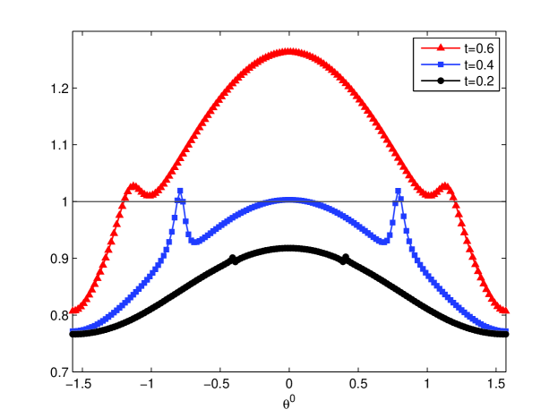
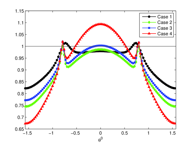
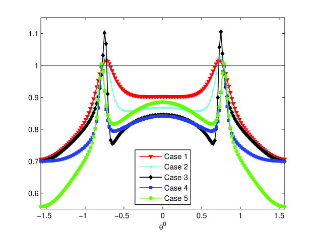
For fixed wave number , the performance of three-level methods is shown in Figure 5. For instance, one can observe from the left graph of Figure 5 that a coarser initial grid used for will deteriorate its convergence. The right graph of Figure 5 shows the spectral radiuses for three kinds of approaches: , and . For , both of and perform better than over most of the frequencies, and the spectral radius of is similar to that of over most of frequencies in this case. Actually, the performance of is always comparable with . This is also true for two-level method, which can be observed from the left graph of Figure 3. Thus, in order to reduce the computational cost, the modified multilevel methods (Algorithm 3.1) with stable CIP-FEM corrections on coarser grids and standard FEM corrections on finer grids can be usually utilized in practical. From the right graph of Figure 5, we can also see that the convergence of does not always perform better with more steps of intermediate coarse grid correction.
5 Numerical results
In this section, we present some numerical results to illustrate the performance of Algorithm 2.1 and modified multilevel method (Algorithm 3.1) for two Helmholtz problems in two dimension. The multilevel method is used as a preconditioner in outer GMRES iterations (PGMRES). Gauss-Seidel relaxation is always used as smoother when , and the smoothing steps are always chosen as one step if there is no any annotation. At the -th level, the discrete problem reads . We denote by the residual with respect to the -th iteration. The PGMRES algorithm terminates when
The number of iteration steps required to achieve the desired accuracy is denoted by iter.
Example 5.1.
We consider a two dimensional Helmholtz equation with the first order absorbing boundary condition (cf. [12, 19]):
Here is a unit square with center and is chosen such that the exact solution is
where are Bessel functions of the first kind.
| Level | 2 | 3 | 4 | 5 |
|---|---|---|---|---|
| DOFs | 16641 | 66049 | 263169 | 1050625 |
| iter (P1) | 27 | 24 | 21 | 20 |
| iter (P2) | 26 | 22 | 19 | 18 |
In this example, we assume that the coarsest level of multilevel method satisfies for . For , we choose the coarsest grid condition such that . The parameters in (2.1) are chosen as (cf. [12]) for CIP-P1, and for piecewise P2 CIP-FEM (CIP-P2). We first test the algorithms for the case with wave number . When Algorithm 2.1 is applied to the discrete system , the smoothing relaxations are all based on the CIP-FEM approximation on fine and coarse grids. Table 1 shows the corresponding iteration counts of PGMRES for discrete system from CIP-P1 and CIP-P2 approximations. We can observe that for fixed the algorithm is robust on different levels.
| Level | 2 | 3 | 4 | 5 | |
|---|---|---|---|---|---|
| DOFs | 16641 | 66049 | 263169 | 1050625 | |
| iter () | 58 | 87 | 94 | 90 | |
| iter () | 46 | 53 | 49 | 47 | |
| Level | 2 | 3 | 4 | 5 | |
| DOFs | 66049 | 263169 | 1050625 | 4198401 | |
| iter (=1) | 177 |
For fixed , when the grid is fine enough to get the accuracy, standard FEM can be utilized again to discretize the problem. But standard multigrid method fails to solve the corresponding discrete system for the case with large wave number. In the following, we mainly apply the multilevel method presented in Algorithm 3.1 with different smoothing strategies. Table 2 shows the iteration counts of this multilevel-preconditioned GMRES method with GMRES smoothing on coarse grids for , and the smoothing relaxations on fine and coarse grids are all based on standard P1 FEM (FEM-P1) approximation. We find that the iteration count is mesh independent for fixed , but it increases rapidly with larger wave number. For instance, for the case with , the iteration counts of PGMRES will be more than 200, even when the GMRES smoothing is performed by steps, the iteration counts are still more than 100. Although more steps of GMRES smoothing can reduce the total iteration counts, it requires more memory to store data in the computation. Actually, the slow convergence of the algorithm mainly lies in the bad approximation on coarse grids. Next, we apply CIP-FEM to construct stable coarse grid corrections.
| Level | 2 | 3 | 4 | 5 |
|---|---|---|---|---|
| DOFs | 16641 | 66049 | 263169 | 1050625 |
| iter (Case 1) | 52 | 64 | 66 | 63 |
| iter (Case 2) | 27 | 24 | 22 | 21 |
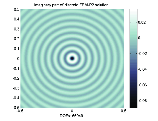
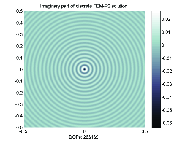
Figure 6 displays the surface plot of imaginary part of discrete FEM-P2 solutions for on the grid with mesh condition . Indeed, the discrete solutions have correct shapes and amplitudes as the exact solutions. Table 3 presents the comparing of shifted Laplace operator with FEM-P1 and the original Helmholtz operator with CIP-P1. For the case , we can see that the second approach has the minimum iteration counts. The iteration counts shown in Table 4 examine the performance of PGMRES based on Algorithm 3.1 with different steps of GMRES smoothing. The CIP-P1 and CIP-P2 are only used for approximations on coarse grids. From Tables 1, 3 and 4, it suggests that Algorithm 3.1 is also very efficient as Algorithm 2.1 and the second approach in Table 3 which uses CIP-FEM on both fine and coarse grids, and the growth in GMRES smoothing steps does not always reduce iteration counts obviously. This supports the similar phenomena shown in the right graph of Figure 5. Hence, in the following we will only use one step () of GMRES smoothing in Algorithm 3.1.
| Level | 3 | 4 | 5 |
|---|---|---|---|
| DOFs | 66049 | 263169 | 1050625 |
| iter (P1, ) | 24 | 23 | 22 |
| iter (P1, ) | 21 | 23 | 23 |
| iter (P2, ) | 27 | 21 | 19 |
| iter (P2, ) | 32 | 21 | 18 |
| Level | 3 | 4 | 5 | |
|---|---|---|---|---|
| DOFs | 16641 | 66049 | 263169 | |
| iter (P1) | 15 | 15 | 15 | |
| iter (P2) | 23 | 14 | 13 | |
| Level | 3 | 4 | 5 | |
| DOFs | 263169 | 1050625 | 4198401 | |
| iter (P1) | 49 | 57 | 55 | |
| iter (P2) | 44 | 41 | 36 | |
| Level | 2 | 3 | 4 | |
| DOFs | 263169 | 1050625 | 4198401 | |
| iter (P1) | 111 | 115 | 112 | |
| iter (P2) | 41 | 44 | 39 |
| FEM-P1 | Level | 2 | 3 | FEM-P2 | Level | 2 | 3 |
|---|---|---|---|---|---|---|---|
| DOFs | 1050625 | 4198401 | DOFs | 1050625 | 4198401 | ||
| iter () | 30 | 26 | iter () | 21 | 14 | ||
| iter () | 71 | 50 | iter () | 29 | 25 | ||
| iter () | 156 | 141 | iter () | 43 | 47 |
Tables 5 and 6 show the iteration counts of PGMRES based on Algorithm 3.1 with CIP-FEM used for correction only on coarse grids for discrete system from FEM-P1 and FEM-P2. For fixed , one can observe that the iteration counts are robust on different levels. Due to the same coarsest grid used for , the growth of iteration counts is a little faster than linear when . But when the FEM-P2 is applied in particular, the growth of iteration counts with increasing wave number is more stable than FEM-P1.
Example 5.2.
In a unit square domain with center , we consider the Helmholtz problem (1.1)-(1.2) with discontinuous wave number, which is defined by
where . We set the Robin boundary condition (1.2) with and the external force to be a narrow Gaussian point source (cf. [7]) located at :
| Level | 3 | 4 | |
|---|---|---|---|
| DOFs | 263169 | 1050625 | |
| iter (P1,) | 26 | 27 | |
| iter (P1,) | 28 | 29 | |
| iter (P2,) | 16 | 15 | |
| iter (P2,) | 17 | 15 | |
| Level | 3 | 4 | |
| DOFs | 1050625 | 4198401 | |
| iter (P1,) | 30 | 30 | |
| iter (P1,) | 32 | 33 | |
| iter (P2,) | 16 | 15 | |
| iter (P2,) | 16 | 15 |
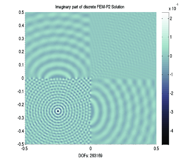
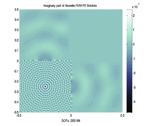
In this example, we test Algorithm 3.1 for the Helmholtz problem with discontinuous wave number. Due to the fact that , the coarsest mesh condition is according to the choice of . Figure 7 displays the surface plot of imaginary part of discrete FEM-P2 solutions for with and on the grid with mesh condition . The iteration counts of PGMRES based on Algorithm 3.1 for different and are listed in Table 7. For fixed and polynomial order, we note that the iteration counts are robust on different levels. Similar to the first example, the PGMRES iteration for FEM-P2 is more stable than FEM-P1.
References
- [1] R. Adams, Sobolev Spaces, Academic Press, New York, 1975.
- [2] A. Brandt, Multi-level adaptive solutions to boundary-value problems, Math. Comp., 31 (1977), pp. 333–390.
- [3] A. Brandt and I. Livshits, Wave-ray multigrid method for standing wave equations, Electron. Trans. Numer. Anal., 6 (1997), pp. 162–181.
- [4] S. Cools and W. Vanroose, Local Fourier Analysis of the Complex Shifted Laplacian preconditioner for Helmholtz problems, preprint, 2011.
- [5] H.C. Elman, O.G. Ernst, and D.P. O’Leary, A multigrid method enhanced by Krylov subspace iteration for discrete Helmholtz equations, SIAM J. Sci. Comput., 23 (2001), pp. 1291–1315.
- [6] B. Engquist and L. Ying, Sweeping preconditioner for the Helmholtz equation: hierarchical matrix representation, Comm. Pure Appl. Math., 64 (2011), pp. 697–735.
- [7] B. Engquist and L. Ying, Sweeping preconditioner for the Helmholtz equation: moving perfectly matched layers, Multiscale Model. Simul., 9 (2011), pp. 686–710.
- [8] Y. A. Erlangga, C. Vuik, and C. W. Oosterlee, On a class of preconditioners for solving the Helmholtz equation, Appl. Numer. Math., 50 (2004), pp. 409–425.
- [9] Y. A. Erlangga, C. W. Oosterlee, and C. Vuik, A novel multigrid based preconditioner for heterogeneous Helmholtz problems, SIAM J. Sci. Comput., 27 (2006), pp. 1471–1492.
- [10] Y.A. Erlangga, Advances in iterative methods and preconditioners for the Helmholtz equation, Arch. Comput. Methods Eng., 15 (2008), pp. 37–66.
- [11] O.G. Ernst and M.J. Gander, Why it is difficult to solve Helmholtz problems with classical iterative methods?, in: I. Graham, T. Hou, O. Lakkis, R. Scheichl (Eds.), Numerical Analysis of Multiscale Problems, Springer, 2011.
- [12] X. Feng and H. Wu, Discontinuous Galerkin methods for the Helmholtz equation with large wave number, SIAM J. Numer. Anal, 47 (2009), pp. 2872–2896.
- [13] X. Feng and H. Wu, hp-discontinuous Galerkin methods for the Helmholtz equation with large wave number, Math. Comp, 80 (2011), pp. 1997–2024.
- [14] F. Ihlenburg, Finite Element Analysis of Acoustic Scattering, Springer-Verlag, New York, 1998.
- [15] S. Kim and S. Kim, Multigrid simulations for high-frequency solutions of the Helmholtz problem in heterogeneous media, SIAM J. Sci. Comput., 24 (2002), pp. 684–701.
- [16] I. Livshits and A. Brandt, Accuracy properties of the wave-ray multigrid algorithm for Helmholtz equations, SIAM J. Sci. Comput., 28 (2006), pp. 1228–1251.
- [17] P.S. Vassilevski and J. Wang, An application of the abstract multilevel theory to nonconforming finite element methods, SIAM J. Numer. Anal., 32 (1995), 235–248.
- [18] R. Wienands and W. Joppich, Practical Fourier Analysis for Multigrid Methods, Chapman & Hall/CRC, London, 2004.
- [19] H. Wu, Pre-asymptotic error analysis of CIP-FEM and FEM for Helmholtz equation with high wave number. Part I: Linear version, to appear, 2013.
- [20] L. Zhu, E. Burman, and H. Wu, Continuous Interior Penalty Finite Element Method for Helmholtz Equation with Large Wave Number: One Dimension Analysis, to appear, 2013.
- [21] L. Zhu and H. Wu, Pre-asymptotic error analysis of CIP-FEM and FEM for Helmholtz equation with high wave number. Part II: version, SIAM J. Numer. Anal., to appear, 2013. (See also arXiv: http://arxiv.org/pdf /1204.5061v1).