Multilevel rejection sampling for approximate Bayesian computation
Abstract
Likelihood-free methods, such as approximate Bayesian computation, are powerful tools for practical inference problems with intractable likelihood functions. Markov chain Monte Carlo and sequential Monte Carlo variants of approximate Bayesian computation can be effective techniques for sampling posterior distributions in an approximate Bayesian computation setting. However, without careful consideration of convergence criteria and selection of proposal kernels, such methods can lead to very biased inference or computationally inefficient sampling. In contrast, rejection sampling for approximate Bayesian computation, despite being computationally intensive, results in independent, identically distributed samples from the approximated posterior. An alternative method is proposed for the acceleration of likelihood-free Bayesian inference that applies multilevel Monte Carlo variance reduction techniques directly to rejection sampling. The resulting method retains the accuracy advantages of rejection sampling while significantly improving the computational efficiency.
1 Introduction
Statistical inference is of fundamental importance to all areas of science. Inference enables the testing of theoretical models against observations, and provides a rational means of quantifying uncertainty in existing models. Modern approaches to statistical inference, based on Monte Carlo sampling techniques, provide insight into many complex phenomena (Beaumont et al., 2002; Pooley et al., 2015; Ross et al., 2017; Stumpf, 2014; Sunnåker et al., 2013; Tavaré et al., 1997; Thorne and Stumpf, 2012; Vo et al., 2015).
Suppose we have: a set of observations, ; a method of determining the likelihood of these observations, , under the assumption of some model characterised by parameter vector ; and a prior probability density, . The posterior probability density, , can be computed using Bayes’ Theorem,
| (1) |
Explicit expressions for likelihood functions are rarely available (Tavaré et al., 1997; Warne et al., 2017; Wilkinson, 2009); motivating the development of likelihood-free methods, such as approximate Bayesian computation (ABC) (Stumpf, 2014; Sunnåker et al., 2013). ABC methods approximate the likelihood through evaluating the discrepancy between data generated by a simulation of the model of interest and the observations, yielding an approximate posterior,
| (2) |
Here, is data generated by the model simulation process, , is a discrepancy metric, and is the acceptance threshold. Due to this approximation, Monte Carlo estimators based on Equation (2) are biased (Barber et al., 2015). In spite of this bias, however, ABC methods have proven to be very powerful tools for practical inference applications in many scientific areas, including evolutionary biology (Beaumont et al., 2002; Tavaré et al., 1997; Thorne and Stumpf, 2012), ecology (Stumpf, 2014), cell biology (Ross et al., 2017; Johnston et al., 2014; Vo et al., 2015) and systems biology (Wilkinson, 2009).
1.1 Sampling algorithms for ABC
The most elementary implementation of ABC is ABC rejection sampling (Pritchard et al., 1999; Sunnåker et al., 2013), see Algorithm 1. This method generates independent and identically distributed samples from the posterior distribution by accepting proposals, , when the data generated by the model simulation process is within of the observed data, , under the discrepancy metric . ABC rejection sampling is simple to implement, and samples are independent and identically distributed. Therefore ABC rejection sampling is widely used in many applications (Browning et al., 2018; Grelaud et al., 2009; Navascués et al., 2017; Ross et al., 2017; Vo et al., 2015). However, ABC rejection sampling can be computationally prohibitive in practice (Barber et al., 2015; Fearnhead and Prangle, 2012). This is especially true when the prior density is highly diffuse compared with the target posterior density (Marin et al., 2012), as most proposals are rejected.
To improve the efficiency of ABC rejection sampling, one can consider a likelihood-free modification of Markov chain Monte Carlo (MCMC) (Beaumont et al., 2002; Marjoram et al., 2003; Tanaka et al., 2006) in which a Markov chain is constructed with a stationary distribution identical to the desired posterior. Given the Markov chain is in state , a state transition is proposed via a proposal kernel, .
The Metropolis-Hastings (Hastings, 1970; Metropolis et al., 1953) state transition probability, , can be modified within an ABC framework to yield
The stationary distribution of such a Markov chain is the desired approximate posterior (Marjoram et al., 2003). Algorithm 2 provides a method for computing iterations of this Markov chain.
While MCMC-ABC sampling can be highly efficient, the samples in the sequence, , are not independent. This can be problematic as it is possible for the Markov chain to take long excursions into regions of low posterior probability. This incurs additional bias that is potentially significant (Sisson et al., 2007). A poor choice of proposal kernel can also have considerable impact upon the efficiency of MCMC-ABC (Green et al., 2015). The question of how to choose the proposal kernel is non-trivial. Typically proposal kernels are determined heuristically. However, automatic and adaptive schemes are available to assist in obtaining near optimal proposals in some cases (Cabras et al., 2015; Roberts and Rosenthal, 2009). Another additional complication is that of determining when the Markov Chain has converged; this is a challenging problem to solve in practice (Roberts and Rosenthal, 2004).
Sequential Monte Carlo (SMC) sampling was introduced to address these potential inefficiencies (Del Moral et al., 2006) and later extended within an ABC context (Sisson et al., 2007; Drovandi and Pettitt, 2011; Toni et al., 2009). A set of samples, referred to as particles, is evolved through a sequence of ABC posteriors defined through a sequence of acceptance thresholds, (Sisson et al., 2007; Beaumont et al., 2009). At each step, , the current ABC posterior, , is approximated by a discrete distribution constructed from a set of particles with importance weights that is, for . The collection is updated to represent the ABC posterior of the next step, , through application of rejection sampling on particles perturbed by a proposal kernel, . If is similar to , the acceptance rate should be high. The importance weights of the new family of particles are updated using an optimal backwards kernel (Sisson et al., 2007; Beaumont et al., 2009). Algorithm 3 outlines the process.
Through the use of independent weighted particles, SMC-ABC avoids long excursions into the distribution tails that are possible with MCMC-ABC. However, SMC-based methods can be affected by particle degeneracy, and the efficiency of each step is still dependent on the choice of proposal kernel (Green et al., 2015; Filippi et al., 2013). Just as with MCMC-ABC, adaptive schemes are available to guide proposal kernel selection (Beaumont et al., 2009; Del Moral et al., 2012). The choice of the sequence of acceptance thresholds is also important for the efficiency of SMC-ABC. However, there are good solutions to generate these sequences in an adaptive manner (Drovandi and Pettitt, 2011; Silk et al., 2013).
1.2 Multilevel Monte Carlo
Multilevel Monte Carlo (MLMC) is a recent development that can significantly reduce the computational burden in the estimation of expectations (Giles, 2008). To demonstrate the basic idea of MLMC, consider computing the expectation of a continuous-time stochastic process at time . Let denote a discrete-time approximation to with time step : the expectations of and are related according to
That is, an estimate of can be treated as a biased estimate of . By taking a sequence of time steps , the indices of which are referred to as levels, we can arrive at a telescoping sum,
| (3) |
Computing this form of the expectation returns the same bias as that returned when computing directly. However, Giles (2008) demonstrates that a Monte Carlo estimator for the telescoping sum can be computed more efficiently than directly estimating in the context of stochastic differential equations (SDEs). This efficiency comes from exploiting the fact that the bias correction terms, , measure the expected difference between the estimates on levels and . Therefore, sample paths of need not be independent of sample paths of . In the case of SDEs, samples may be generated in pairs driven by the same underlying Brownian motion, that is, the pair is coupled. By the strong convergence properties of numerical schemes for SDEs, Giles (2008) shows that this coupling is sufficient to reduce the variance of the Monte Carlo estimator. This reduction in variance is achieved through optimally trading off statistical error and computational cost across all levels. Through this trade-off, an estimator is obtained with the same accuracy in mean-square to standard Monte Carlo, but at a reduced computational cost. This saving of computational cost is achieved since fewer samples of the most accurate discretisation are required.
1.3 Related work
Recently, several examples of MLMC applications to Bayesian inference problems have appeared in the literature. One of the biggest challenges in the application of MLMC to inverse problems is the introduction of a strong coupling between levels. That is, the construction of a coupling mechanism that reduces the variances of the bias correction terms enough to enable the MLMC estimator to be computed more efficiently than standard Monte Carlo. Dodwell et al. (2015) demonstrate a MLMC scheme for MCMC sampling applicable to high-dimensional Bayesian inverse problems with closed-form likelihood expressions. The coupling of Dodwell et al. (2015) is based on correlating Markov chains defined on a hierarchy in parameter space. A similar approach is also employed by Efendiev et al. (2015). A multilevel method for ensemble particle filtering is proposed by Gregory et al. (2016) that employs an optimal transport problem to correlate a sequence of particle filters of different levels of accuracy. Due to the computational cost of the transport problem, a local approximation scheme is introduced for multivariate parameters (Gregory et al., 2016). Beskos et al. (2017) look more generally at the case of applying MLMC methods when independent and identically distributed sampling of the distributions on some levels is infeasible, the result is an extension of MLMC in which coupling is replaced with sequential importance sampling, that is, a multilevel variant of SMC (MLSMC).
MLMC has also recently been considered in an ABC context. Guha and Tan (2017) extend the work of Efendiev et al. (2015) by replacing the Metropolis-Hasting acceptance probability in a similar way to the MCMC-ABC method (Marjoram et al., 2003). The MLSMC method (Beskos et al., 2017) is exploited to achieve coupling in an ABC context by Jasra et al. (2017).
1.4 Aims and contribution
ABC samplers based on MCMC and SMC are generally more computationally efficient than ABC rejection sampling (Marjoram et al., 2003; Sisson et al., 2007; Toni et al., 2009). However, there are many advantages to using ABC rejection sampling. Specific advantages are: (i) its simple implementation; (ii) it produces truly independent and identically distributed samples, that is, there is no need to re-weight samples; and (iii) there are no algorithm parameters that affect the computational efficiency. In particular, no proposal kernels need be heuristically defined for ABC rejection sampling.
The aim of this work is to design a new algorithm for ABC inference that retains the aforementioned advantages of ABC rejection sampling, while still being efficient and accurate. The aim is not to develop a method that is always superior to MCMC and SMC methods, but rather provide a method that requires little user-defined configuration, and is still computationally reasonable. To this end, we investigate MLMC methods applied directly to ABC rejection sampling.
Various applications of MLMC to ABC inference have been demonstrated very recently in the literature (Guha and Tan, 2017; Jasra et al., 2017), with each implementation contributing different ideas for constructing effective control variates in an ABC context. It is not yet clear when one approach will be superior to another. Thus the question of how best to apply MLMC in an ABC context remains an open problem. Since there are no examples of an application of MLMC methods to the most fundamental of ABC samplers, that is rejection sampling, such an application is a significant contribution to this field.
We describe a new algorithm for ABC rejection sampling, based on MLMC. Our new algorithm, called MLMC-ABC, is as general as standard ABC rejection sampling but is more computationally efficient through the use of variance reduction techniques that employ a novel construction for the coupling problem. We describe the algorithm, its implementation, and validate the method using a tractable Bayesian inverse problem. We also compare the performance of the new method against MCMC-ABC and SMC-ABC using a standard benchmark problem from epidemiology.
Our method benefits from the simplicity of ABC rejection sampling. We require only the discrepancy metric and a sequence of acceptance thresholds to be defined for a given inverse problem. Our approach is also efficient, and achieves comparable or superior performance to MCMC-ABC and SMC-ABC methods, at least for the examples considered in this paper. Therefore, we demonstrate that our algorithm is a promising method that could be extended to design viable alternatives to current state-of-the-art approaches. This work, along with that of Guha and Tan (2017) and Jasra et al. (2017), provides an additional set of computational tools to further enhance the utility of ABC methods in practice.
2 Methods
In this section, we demonstrate our application of MLMC ideas to the likelihood-free inference problem given in Equation (2). The initial aim is to compute an accurate approximation to the joint posterior cumulative distribution function (CDF) of , using as few data generation steps as possible. We define a data generation step to be a simulation of the model of interest given a proposed parameter vector. While the initial presentation is given in the context of estimating the joint CDF, the method naturally extends to expectations of other functions (see A). However, the joint CDF is considered first for clarity in the introduction of the MLMC coupling strategy.
We apply MLMC methods to likelihood-free Bayesian inference by reposing the problem of computing the posterior CDF as an expectation calculation. This allows the MLMC telescoping sum idea, as in Equation (3), to be applied. In this context, the levels of the MLMC estimator are parameterised by a sequence of acceptance thresholds with for all . The efficiency of MLMC relies upon computing the terms of the telescoping sum with low variance. Variance reduction is achieved through exploiting features of the telescoping sum for CDF approximation, and further computational gains are achieved by using properties of nested ABC rejection samplers.
2.1 ABC posterior as an expectation
We first reformulate the Bayesian inference problem (Equation (1)) as an expectation. To this end, note that, given a -dimensional parameter space, , and the random parameter vector, , if the joint posterior CDF, is differentiable, that is, its probability density function (PDF) exists, then
where . This can be expressed as an expectation by noting
where is the indicator function: whenever and otherwise. Now, consider the ABC approximation given in Equation (2) with discrepancy metric and acceptance threshold . The ABC posterior CDF, denoted by , will be
| (4) |
The marginal ABC posterior CDFs, , are
2.2 Multilevel estimator formulation
We now introduce some notation that will simplify further derivations. We define to be a random vector distributed according to the ABC posterior CDF, , with acceptance threshold, , as given in Equation (2.1). This provides us with simplification in notation for the ABC posterior PDF, , and the conditional expectation, . For any expectation, , we use to denote the Monte Carlo estimate of this expectation using samples.
The standard Monte Carlo integration approach is to generate samples from the ABC posterior, , then evaluate the empirical CDF (eCDF),
| (5) |
for , where is a discretisation of the parameter space . For simplicity, we will consider to be a -dimensional regular lattice. In general, a regular lattice will not be well suited for high dimensional problems. However, since this is the first time that this MLMC approach has been presented, it is most natural to begin the exposition with a regular lattice, and then discuss other more computationally efficient approaches later. More attention is given to other possibilities in Section 4.
The eCDF is not, however, the only Monte Carlo approximation to the CDF one may consider. In particular, Giles et al. (2015) demonstrate the application of MLMC to a univariate CDF approximation. We now present a multivariate equivalent of the MLMC CDF of Giles et al. (2015) in the context of ABC posterior CDF estimation. Consider a sequence of acceptance thresholds, , that is strictly decreasing, that is, . In this work, the problem of constructing optimal sequences is not considered, as the focus is the initial development of the method. More discussion around this problem is given in Section 4. Given such a sequence, , we can represent the CDF (Equation (2.1)) using the telescoping sum
| (6) |
where
| (7) |
Using our notation, the MLMC estimator for Equation (6) and Equation (7) is given by
| (8) |
where
| (9) |
and is a Lipschitz continuous approximation to the indicator function; this approximation is computed using a tensor product of cubic polynomials,
where is the lattice spacing in the th dimension, and is a piece-wise continuous polynomial,
This expression is based on the rigorous treatment of smoothing required in the univariate case given by Giles et al. (2015). While other polynomials that satisfy certain conditions are possible (Giles et al., 2015; Reiss, 1981), here we restrict ourselves to this relatively simple form. Application of the smoothing function improves the quality of the final CDF estimate, just as using smoothing kernels improves the quality of PDF estimators (Silverman, 1986). Such a smoothing is also necessary to avoid convergence issues with MLMC caused by the discontinuity of the indicator function (Avikainen, 2009; Giles et al., 2015).
To compute the term (Equation (9)), we generate samples from ; this represents a biased estimate for . To compensate for this bias, correction terms, , are evaluated for , each requiring the generation of samples from and samples from , as given in Equation (9). It is important to note that the samples, , used to compute are independent of the samples, , used to compute .
2.3 Variance reduction
The goal is to introduce a coupling between levels that controls the variance of the bias correction terms. With an effective coupling, the result is an estimator with lower variance, hence the number of samples required to obtain an accurate estimate is reduced. Denote as the variance of the estimator . For this can be expressed as
where and denote the variance and covariance, respectively. Introducing a positive correlation between the random variables and will have the desired effect of reducing the variance of .
In many applications of MLMC, a positive correlation is introduced through driving samplers at both the and level with the same randomness. Properties of Brownian motion or Poisson processes are typically used for the estimation of expectations involving SDEs or Markov processes (Giles, 2008; Anderson and Higham, 2012; Lester et al., 2016). In the context of ABC methods, however, simulation of the quantity of interest is necessarily based on rejection sampling. The reliance on rejection sampling makes a strong coupling, in the true sense of MLMC, a difficult, if not impossible task. Rather, here we introduce a weaker form of coupling through exploiting the fact that our MLMC estimator is performing the task of computing an estimate of the ABC posterior CDF. We combine this with a property of nested ABC rejection samplers to arrive at an efficient algorithm for computing .
We proceed to establish a correlation between levels as follows. Assume we have computed, for some , the terms in Equation (8). That is, we have an estimator to the CDF at level by taking the sum
with marginal distributions for . We can use this to determine a coupling based on matching marginal probabilities when computing . After generating samples from , we compute the eCDF, , using Equation (5) and obtain the marginal distributions, for . We can thus generate coupled pairs by choosing the with the same marginal probabilities as the empirical probability of . That is, the th component of is given by
where is the th component of and is the inverse of the th marginal distribution of . This introduces a positive correlation between the sample pairs, , since an increase in any of the components of will cause an increase in the same component . This correlation reduces the variance in the bias correction estimator computed according to Equation (9). We can then update the MLMC CDF to get an improved estimator by using
and apply an adjustment that ensures monotonicity. We continue this process iteratively to obtain .
It must be noted here that this coupling mechanism introduces an approximation for the general inference problem; therefore some additional bias can be introduced. This is made clear when one considers the process in terms of the copula distributions of and . If these copula distributions are the same, then the coupling is exact and there is no additional bias. The coupling is also exact for the univariate case (). Therefore, under the assumption that the correlation structure does not change significantly between levels, then the bias should be low. In practice, this requirement affects the choice of the acceptance threshold sequence, ; we discuss this in more detail in Section 4. In Section 3.1, we demonstrate that for sensible choices of this sequence, the introduced bias is small compared with the bias that is inherent in the ABC approximation.
2.4 Optimal sample sizes
We now require the sample numbers that are the optimal trade-off between accuracy and efficiency. Denote as the number of data generation steps required during the computation of and let be the average number of data generation steps per accepted ABC posterior sample using acceptance threshold .
Given and , for , one can construct the optimal under the constraint , where is the target variance of the MLMC CDF estimator. As shown by Giles (2008), using a Lagrange multiplier method, the optimal are given by
| (10) |
In practice, the values for and will not have analytic expressions available; rather, we perform a low accuracy trial simulation with all , for some comparatively small constant, , to obtain the relative scaling of variances and data generation requirements.
2.5 Improving acceptance rates
A MLMC method based on the estimator in Equation (8) and the variance reduction strategy given in Section 2.3 would depend on standard ABC rejection sampling (Algorithm 1) for the final bias correction term . For many ABC applications of interest, the computation of this final term will dominate the computational costs. Therefore, the potential computational gains depend entirely on the size of compared to the number of samples, , required for the equivalent standard Monte Carlo approach (Equation (5)). While this approach is often an improvement over rejection sampling, we can achieve further computational gains by exploiting the iterative computation of the bias correction terms.
Let denote the support of a function , and note that, for any , . This follows from the fact that if, for any , , then since . That is, any simulated data generated using parameter values taken from outside cannot be accepted on level since almost surely. Therefore, we can truncate the prior to the support of when computing , thus increasing the acceptance rate of level samples. In practice, we need to approximate the support regions through sampling. For simplicity, in this work we restrict sampling of the prior at level to within the bounding box that contains all the samples generated at level . However, more sophisticated approaches could be considered, and may result in further computational improvements.
2.6 The algorithm
We now have all the components to construct our MLMC-ABC algorithm. We compute the MLMC CDF estimator (Equation (8)) using the coupling technique for the bias correction terms (Section 2.3) and prior truncation for improved acceptance rates (Section 2.5).
Optimal are estimated as per Equation (10) and Section 2.4. Once have been estimated, computation of the MLMC-ABC posterior CDF proceeds according to Algorithm 4.
The computational complexity of MLMC-ABC (Algorithm 4) is roughly where is the expected cost of generating a single sample of the ABC posterior with threshold , is the cost of updating the CDF estimate and is the cost of the coupling which involves the marginal CDF inverses. From Algorithm 4, we have and from Barber et al. (2015) we have where is the dimensionality of . The marginal inverse operations require only two steps:
-
1.
find such that, . Such an operation is, at most, ;
-
2.
invert the interpolating cubic spline, which can be done in .
It follows that . For any practical application, will need to be sufficiently small, that is, , in order for the cost of generating posterior samples at level dominates the cost of the marginal CDF inverse operations and the lattice updating. Computational gains over ABC rejection sampling are achieved through decreasing and , via variance reduction and prior truncation.
Our primary focus in Algorithm 4 is on using MLMC to estimate the posterior CDF. The coupling mechanism is more readily communicated in this case. However, the MLMC-ABC method is more general and can be used to estimate where is any Lipschitz continuous function. In this more general case, only the marginal CDFs need be accumulated to facilitate the coupling mechanism. For more details see A.
3 Results
In this section, we provide numerical results to demonstrate the validity, accuracy and performance of our MLMC-ABC method using some common models from epidemiology. In the first instance, we consider a tractable compartmental model, the stochastic SIS (Susceptible-Infected-Susceptible) model (Weiss and Dishon, 1971), to confirm the convergence and accuracy of MLMC-ABC. We then consider the Tuberculosis transmission model introduced by Tanaka et al. (2006) as a benchmark to compare our method with MCMC-ABC (Algorithm 2) and SMC-ABC (Algorithm 3). While we have chosen to perform our evaluation using an epidemiological model due to the particular prevalence of ABC methods in the life sciences, the techniques outlined in this manuscript are completely general and applicable to many areas of science.
3.1 A tractable example
The SIS model is a common model from epidemiology that describes the spread of a disease or infection for which no significant immunity is obtained after recovery; the common cold, for example. The model is given by
with parameters and hazard functions for infection and recovery given by
respectively. This process defines a discrete-state continuous-time Markov process with a forward transitional density function that is computationally feasible to evaluate exactly for small populations . That is, for , the probability of given , with density denoted by , has a solution obtained through the th element of the vector
| (11) |
where the th element of column vector, , is one and all other elements zero, denotes the matrix exponential and is the infinitesimal generator matrix of the Markov process; for the SIS model, is a tri-diagonal matrix dependent only on the parameters of the model.
Let be an observation at time of the number of susceptible individuals in the population. We generate observations using a single realisation of the SIS model with parameters and , population size , and initial conditions and ; Observations are taken at times . Using the analytic solution to the SIS transitional density (using Equation (11)), we arrive at the likelihood function
| (12) |
where almost surely. Hence, we can obtain an exact solution to the SIS posterior given the priors and . Given this exact posterior, quadrature can be applied to compute the posterior CDF, given by
For the ABC approximation we use a discrepancy metric based on the sum of squared errors,
where is a realisation of the model generated using the Gillespie algorithm (Gillespie, 1977) for a given set of parameters, and . An appropriate acceptance threshold sequence for this metric is , with , and (Toni et al., 2009).
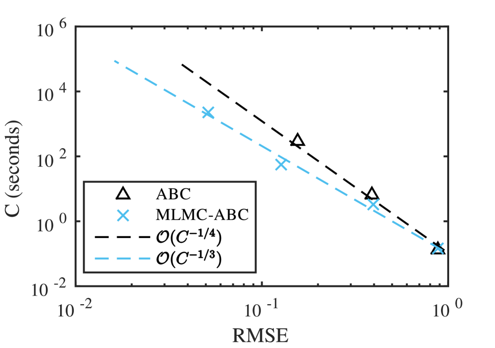
We can use the exact likelihood (Equation (12)) to evaluate the convergence properties of our MLMC-ABC method. Based on the analysis of ABC rejection sampling by Barber et al. (2015), the rate of decay of the root mean-squared error (RMSE) as the computational cost is increased is slower for ABC than standard Monte Carlo. We find experimentally for ABC rejection sampling, that the decay of RMSE of the SIS model is approximately , where is the expected computational cost of generating ABC posterior samples. The confidence interval of this experimental rate is , which is consistent with the expected theoretical result of (Barber et al., 2015). This is slower than the expected decay typically achieved with standard Monte Carlo. We compare the ABC rejection sampler decay rate with that achieved by our MLMC-ABC methods.
We use the norm for the RMSE, that is,
where is the exact posterior CDF, evaluated directly from the likelihood (Equation (12)), and is the Monte Carlo estimate of the CDF. A regular lattice that consists of points is used for this estimate. The computation required for Gillespie simulations completely dominates the added computation of updating the lattice. The RMSE is computed using independent MLMC-ABC CDF estimations for . The sequence of sample numbers, , is computed using Equation (10) with target variance of and trial samples. Figure 1 demonstrates the improved convergence rate over the ABC rejection sampler convergence rate. Based on the least-squares fit, the RMSE decay is approximately . The confidence interval for the rate is which is consistent with theory from Giles et al. (2015) for the univariate situation. For smaller target RMSE, this results in an order of magnitude reduction in the computational cost.
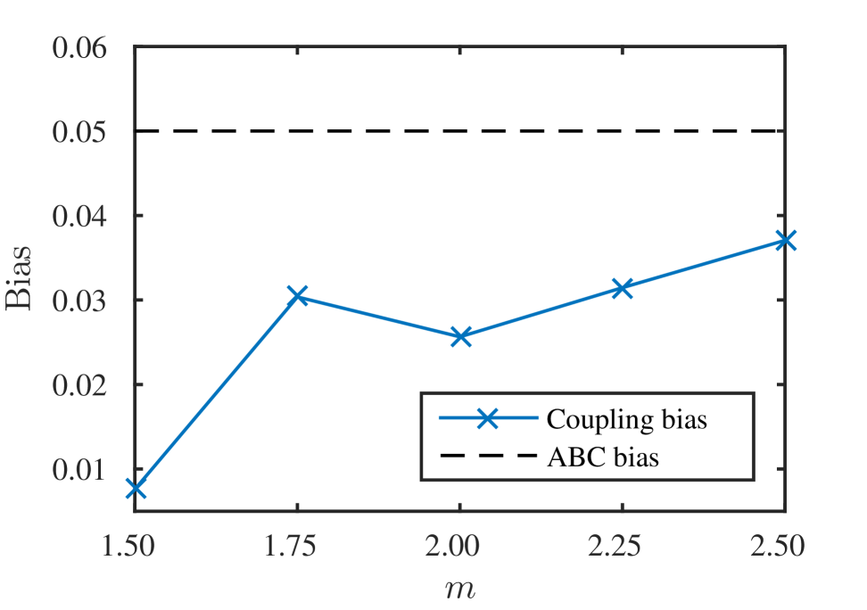
We also consider the effect of the additional bias introduced through the coupling mechanism as presented in Section 2.3. We set the sample numbers at all levels to be to ensure the Monte Carlo error is negligible and compare the bias for different values of acceptance threshold scaling factor . The bias is computed according to the norm, that is,
where denotes the estimator computed according to Algorithm 4 and denotes the estimator computed without any coupling. That is, is computed using standard Monte Carlo to evaluate each term in the MLMC telescoping sum (Equation (6)). Note that, computationally, will always be inferior to a standard Monte Carlo estimate. Figure 2 shows that, not only does the bias decay as decreases, but also the additional bias is well within the order of bias expected from the ABC approximation. This result, along with Figure 1, demonstrates that the reduction in estimator variance can dominate the increase in bias. Thus, compared with standard Monte Carlo, a significantly lower RMSE for the same computational effort is achieved with MLMC using this coupling strategy.
3.2 Performance evaluation
We now evaluate the performance of MLMC-ABC using the model developed by Tanaka et al. (2006) in the study of tuberculosis transmission rate parameters using DNA fingerprint data (Small et al., 1994). This model has been selected due to the availability of published comparative performance evaluations of MCMC-ABC and SMC-ABC (Tanaka et al., 2006; Sisson et al., 2007).
The model proposed by Tanaka et al. (2006) describes the occurrence of tuberculosis infections over time and the mutation of the bacterium responsible, Myobacterium tuberculosis. The number of infections, , at time is
where is the number of distinct genotypes and is the number of infections caused by the th genotype at time . For each genotype, new infections occur with rate , infections terminate with rate , and mutation occurs with rate ; causing an increase in the number of genotypes. This process, as with the SIS model, can be described by a discrete-state continuous-time Markov process. In this case, however, the likelihood is intractable, but the model can still be simulated using the Gillespie algorithm (Gillespie, 1977). After a realisation of the model is completed, either by extinction or when a maximum infection count is reached, a sub-sample of cases is collected and compared against the IS DNA fingerprint data of tuberculosis bacteria samples (Small et al., 1994). The dataset consists of distinct genotypes; the infection cases are clustered according to the genotype responsible for the infection. The collection of clusters can be summarised succinctly as where denotes there are clusters of size . The discrepancy metric used is
| (13) |
where is the size of the population sub-sample (e.g., ), denotes the number of distinct genotypes in the dataset (e.g., ) and the genetic diversity is
where is the cluster size of the th genotype in the dataset.
We perform likelihood-free inference on the tuberculosis model for the parameters with the goal of evaluating the efficiencies of MLMC-ABC, MCMC-ABC and SMC-ABC. We use a target posterior distribution of with as defined in Equation (13) and . The acceptance threshold sequence, , used for both SMC-ABC and MLMC-ABC is with and . The improper prior is given by , and (Sisson et al., 2007; Tanaka et al., 2006). For the MCMC-ABC and SMC-ABC algorithms we apply a typical Gaussian proposal kernel,
with covariance matrix
| (14) |
Such a proposal kernel is reasonable to characterise the initial explorations of an ABC posterior as no correlations between parameters are assumed.
While MLMC-ABC does not require a proposal kernel function, some knowledge of the variance of each bias correction term is needed to determine the optimal sample numbers, . This is achieved using trial samples of each level. The number of data generation steps is also recorded to compute , as per Equation (10). The resulting sample numbers are then scaled such that is a user prescribed value.
The efficiency metric we use is the root mean-squared error (RMSE) of the CDF estimate versus the total number of data generation steps, . The mean-squared error (MSE) is taken under the norm, that is, where is the exact ABC posterior CDF and is the Monte Carlo estimate using a regular lattice with points. To compute the RMSE, a high precision solution is computed using ABC rejection samples of the target ABC posterior. This is computed over a period of 48 hours using 500 processor cores.
Table 1 presents the RMSE for MCMC-ABC, SMC-ABC and MLMC-ABC for different configurations. The RMSE values are computed using 10 independent estimator calculations. The algorithm parameter varied is the number of particles, , for SMC-ABC, the number of iterations, , for MCMC-ABC and the level sample number, , for MLMC-ABC.
| MLMC-ABC | MCMC-ABC | SMC-ABC | ||||||
|---|---|---|---|---|---|---|---|---|
| RMSE | RMSE | RMSE | ||||||
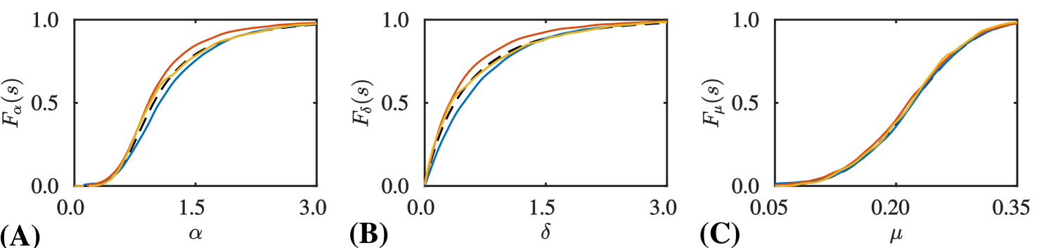
Using the proposal kernel provided in Equation (14), SMC-ABC requires almost more data generation steps than MLMC-ABC to obtain the same RMSE. MLMC-ABC obtains nearly double the accuracy of MCMC-ABC for the same number of data generation steps. Figure 3 shows an example of the high precision marginal posterior CDFs, , and , compared with the numerical solutions computed using the three methods.
We note that these results represent a typical scenario when solving this problem with a standard choice of proposal densities for MCMC-ABC and SMC-ABC. However, obtaining a good proposal kernel is a difficult open problem, and infeasible to do heuristically for high-dimensional parameter spaces. Therefore, efficient proposal kernels are almost never obtained without significant manual adjustment or additional algorithmic modifications such as adaptive schemes (Beaumont et al., 2009; Del Moral et al., 2012; Roberts and Rosenthal, 2009). Nevertheless, we demonstrate in Table 2 the increased efficiency for MCMC-ABC and SMC-ABC when using a highly configured Gaussian proposal kernel with covariance matrix as determined by Tanaka et al. (2006)
| (15) |
| MLMC-ABC | MCMC-ABC | SMC-ABC | ||||||
|---|---|---|---|---|---|---|---|---|
| RMSE | RMSE | RMSE | ||||||
We note that Sisson et al. (2007) use a similar proposal kernel, however they do not explicitly state the difference in the covariance matrix ; we therefore assume that Equation (15) represents a proposal kernel that is heuristically optimal to the target posterior density. We emphasise that it would be incredibly rare to arrive at an optimal proposal kernel without any additional experimentation. Even in this unlikely case, MLMC-ABC is still comparable with MCMC-ABC. However, MLMC-ABC is clearly not as efficient as SMC-ABC for this heuristically optimised scenario. The scenario is intentionally biased toward MCMC-ABC and SMC-ABC, so this result is not unexpected. Future research could consider a comparison of the methods when the extra computational burden of determining the optimal , such as implementation of an adaptive scheme, is taken into account.
4 Discussion
Our results indicate that, while SMC-ABC and MCMC-ABC can be heuristically optimised to be highly efficient, an accurate estimate of the parameter posterior can be obtained using the MLMC-ABC method presented here in a relatively automatic fashion. Furthermore, the efficiency of MLMC-ABC is comparable or improved over MCMC-ABC and SMC-ABC, even in the case when efficient proposal kernels are employed.
The need to estimate the variances of each bias correction term could be considered a limitation of the MLMC-ABC approach. However, we find in practice that these need not be computed to high accuracy and can often be estimated with a relatively small number of samples. There could be examples of Bayesian inference problems where MLMC-ABC is inefficient on account of the variance estimation inaccuracy. We have so far, however, failed to find an example for which samples of each bias correction term is insufficient to obtain a good MLMC-ABC estimator.
There are many modifications one could consider to further improve MLMC-ABC. In this work, we explicitly specify the sequence of acceptance thresholds in advance for both MLMC-ABC and SMC-ABC. As this is the initial presentation of the method, it is appropriate to consider this idealised case. However, it is unclear if an optimal sequence of thresholds for SMC-ABC will also be optimal for MLMC-ABC and vice versa. Furthermore, as mention in Section 1, practical applications of SMC-ABC often determine such sequences adaptively (Drovandi and Pettitt, 2011; Silk et al., 2013). A modification of MLMC-ABC to allow for adaptive acceptance thresholds would make MLMC-ABC even more practical as it could be used to minimise the coupling bias. The exact mechanisms to achieve this could be based on similar ideas to adaptive SMC-ABC (Drovandi and Pettitt, 2011). Given the solution at level , the next level could be determined through: (i) sampling a fixed set of prior samples; (ii) sorting these samples based on the discrepancy metric; (iii) selecting a discrepancy threshold, , that optimises coupling bias and the variance of the bias correction term. Future work should address these open problems.
Other improvements could focus on the discretisation used for the eCDF calculations. The MLMC-ABC method has no requirement of a regular lattice, and alternative choices would likely enable MLMC-ABC to scale to much higher dimensional parameter spaces. Adaptive grids that refine with each level is one option that could be considered; however, unstructured grids or kernel based methods also have potential.
Improvements to the coupling scheme are also possible avenues for future consideration. The coupling approach we have considered depends only on the computation of the marginal posterior CDFs and assumes nothing about the underlying model. It may be possible to take advantage of certain model specific features to improve variance reduction. There may also be cases where the rejection sampling scheme is prohibitive for the more accurate acceptance levels. The combination of our coupling scheme with the MLSMC scheme recently proposed by Beskos et al. (2017) and Jasra et al. (2017) is a promising possibility to mitigate these issues. Future work should investigate, compare and contrast the variety of available coupling strategies in the growing body of literature on MLMC for ABC and Bayesian inverse problems.
We have shown, in a practical way, how MLMC techniques can be applied to ABC inference. We also demonstrate that variance reduction strategies, even when applied to simple methods such as rejection sampling, can achieve performance improvements comparable, and in some cases superior, to modern advanced ABC methods based on MCMC and SMC methods. Therefore, the MLMC framework is a promising area for designing improved samplers for complex statistical problems with intractable likelihoods.
Acknowledgements
This work is supported by the Australian Research Council (FT130100148). REB would like to thank the Royal Society for a Royal Society Wolfson Research Merit Award and the Leverhulme Trust for a Leverhulme Research Fellowship. REB would also like to acknowledge support from the Biotechnology and Biological Sciences Research Council (BB/R000816/1). Computational resources were provided by High Performance Computing and Advanced Research Computing support (HPC-ARCs), Queensland University of Technology (QUT). The authors thank Mike Giles and Chris Drovandi for helpful discussions, and two anonymous reviewers and the Associate Editor for insightful comments and suggestions.
Appendix A MLMC for ABC with general Lipschitz functions
Minor modifications of the MLMC-ABC method (Algorithm 4) are possible to enable the computation of expectations of the form
where is any Lipschitz continuous function.
Using the same notation as defined in Section 2.2, the MLMC telescoping sum may be formed for a given sequence of acceptance thresholds, , to compute the expectation . That is,
| (16) |
From Equation (16), it is straightforward to obtain equivalent expressions to Equation (8) and Equation (9).
The modified MLMC-ABC algorithm proceeds in a very similar fashion to Algorithm 4, however, there is no need to hold a complete discretisation of the parameter space, . This is because only the marginal CDFs, , are required to form the coupling strategy in Section 2.3. Thus, we denote to be a discretisation of the th coordinate axis. This significantly reduces the computational burden of the lattice in higher dimensions since . The resulting algorithm is given in Algorithm 5.
References
- Anderson and Higham (2012) Anderson, D.F., Higham, D.J., 2012. Multilevel Monte Carlo for continuous time Markov chains, with applications in biochemical kinetics. Multiscale Modeling & Simulation 10(1):146–179. DOI 10.1137/110840546
- Avikainen (2009) Avikainen, R., 2009. On irregular functionals of SDEs and the Euler scheme. Finance and Stochastics 13(3):381–401. DOI 10.1007/s00780-009-0099-7
- Barber et al. (2015) Barber, S., Voss, J., Webster, M., 2015. The rate of convergence for approximate Bayesian computation. Electronic Journal of Statistics 9:80–105. DOI 10.1214/15-EJS988
- Beaumont et al. (2002) Beaumont, M.A., Zhang, W., Balding, D.J., 2002. Approximate Bayesian computation in population genetics. Genetics 162(4):2025–2035.
- Beaumont et al. (2009) Beaumont, M.A., Cornuet, J.M., Marin, J.M., Robert, C.P., 2009. Adaptive approximate Bayesian computation. Biometrika 96(4):983–990.
- Beskos et al. (2017) Beskos, A., Jasra, A., Law, K., Tempone, R., Zhou, Y., 2017. Multilevel sequential Monte Carlo samplers. Stochastic Processes and their Applications 127(5):1417–1440. DOI 10.1016/j.spa.2016.08.004
- Browning et al. (2018) Browning, A.P., McCue, S.W., Binny, R.N., Plank, M.J., Shah, E.T., Simpson, M.J., 2018. Inferring parameters for a lattice-free model of cell migration and proliferation using experimental data. Journal of Theoretical Biology 437:251–260. DOI 10.1016/j.jtbi.2017.10.032
- Cabras et al. (2015) Cabras, S., Castellanos Neuda, M.E., Ruli, E., 2015. Approximate Bayesian computation by modelling summary statistics in a quasi-likelihood framework. Bayesian Analysis 10(2):411–439. DOI 10.1214/14-BA921
- Del Moral et al. (2006) Del Moral, P., Doucet, A., Jasra, A., 2006. Sequential Monte Carlo samplers. Journal of the Royal Statistical Society: Series B (Statistical Methodology) 68(3):411–436. DOI 10.1111/j.1467-9868.2006.00553.x
- Del Moral et al. (2012) Del Moral, P., Doucet, A., Jasra, A., 2012. An adaptive sequential Monte Carlo method for approximate Bayesian computation. Statistics and Computing 22(5):1009–1020. DOI 10.1007/s11222-011-9271-y
- Dodwell et al. (2015) Dodwell, T.J., Ketelsen, C., Scheichl, R., Teckentrup, A.L., 2015. A hierarchical multilevel Markov chain Monte Carlo algorithm with applications to uncertainty quantification in subsurface flow. SIAM/ASA Journal on Uncertainty Quantification 3(1):1075–1108. DOI 10.1137/130915005
- Drovandi and Pettitt (2011) Drovandi, C.C., Pettitt, A.N., 2011. Estimation of parameters for macroparasite population evolution using approximate Bayesian computation. Biometrics 67(1):225–233. DOI 10.1111/j.1541-0420.2010.01410.x
- Efendiev et al. (2015) Efendiev, Y., Jin, B., Michael, P., Tan, X., 2015. Multilevel Markov chain Monte Carlo method for high-contrast single-phase flow problems. Communications in Computational Physics 17(1):259–286. DOI 10.4208/cicp.021013.260614a
- Fearnhead and Prangle (2012) Fearnhead, P., Prangle, D., 2012. Constructing summary statistics for approximate Bayesian computation: semi-automatic approximate Bayesian computation. Journal of the Royal Statistical Society Series B (Statistical Methodology) 74(3):419–474. DOI 10.1111/j.1467-9868.2011.01010.x
- Filippi et al. (2013) Filippi, S., Barnes, C.P., Cornebise, J., Stumpf, M.P.H., 2013. On optimality of kernels for approximate Bayesian computation using sequential Monte Carlo. Statistical Applications in Genetics and Molecular Biology 12(1):87–107. DOI 10.1515/sagmb-2012-0069
- Giles (2008) Giles, M.B., 2008. Multilevel Monte Carlo path simulation. Operations Research 56(3):607–617. DOI 10.1287/opre.1070.0496
- Giles et al. (2015) Giles, M.B., Nagapetyan, T., Ritter, K., 2015. Multilevel Monte Carlo approximation of cumulative distribution function and probability densities. SIAM/ASA Journal on Uncertainty Quantification 3(1):267–295. DOI 10.1137/140960086
- Gillespie (1977) Gillespie, D.T., 1977. Exact stochastic simulation of coupled chemical reactions. The Journal of Physical Chemistry 81(25):2340–2361. DOI 10.1021/j100540a008
- Green et al. (2015) Green, P.J., Łatuszyński, K., Pereyra, M., Robert, C.P., 2015. Bayesian computation: a summary of the current state, and samples backwards and forwards. Statistics and Computing 25(4):835–862. DOI 10.1007/s11222-015-9574-5
- Gregory et al. (2016) Gregory, A., Cotter, C.J., Reich, S., 2016. Multilevel ensemble transform particle filtering. SIAM Journal on Scientific Computing 38(3):A1317–A1338. DOI 10.1137/15M1038232
- Grelaud et al. (2009) Grelaud, A., Marin, J.-M., Robert, C.P., Rodolphe, F., Tallay, J.-F., 2009. ABC likelihood-free methods for model choice in Gibbs random fields. Bayesian Analysis 4(2):317–335. DOI 10.1214/09-BA412
- Guha and Tan (2017) Guha, N., Tan, X., 2017. Multilevel approximate Bayesian approaches for flows in highly heterogeneous porous media and their applications. Journal of Computational and Applied Mathematics 317:700 – 717. DOI 10.1016/j.cam.2016.10.008
- Hastings (1970) Hastings, W.K., 1970. Monte Carlo sampling methods using Markov chains and their applications. Biometrika 57(1):97–109.
- Jasra et al. (2017) Jasra, A., Jo, S., Nott, D., Shoemaker, C., Tempone, R., 2017. Multilevel Monte Carlo in approximate Bayesian computation. ArXiv e-prints URL https://arxiv.org/abs/1702.03628, 1702.03628.
- Johnston et al. (2014) Johnston, S.T., Simpson, M.J., McElwain, D.L.S., Binder, B.J., Ross, J.V., 2014 Interpreting scratch assays using pair density dynamics and approximate Bayesian computation. Open Biology 4(9):140097. DOI 10.1098/rsob.140097
- Lester et al. (2016) Lester, C., Baker, R.E., Giles, M.B., Yates, C.A., 2016. Extending the multi-level method for the simulation of stochastic biological systems. Bulletin of Mathematical Biology 78(8):1640–1677. DOI 10.1007/s11538-016-0178-9
- Marjoram et al. (2003) Marjoram, P., Molitor, J., Plagnol, V., Tavaré, S., 2003. Markov chain Monte Carlo without likelihoods. Proceedings of the National Academy of Sciences of the United States of America 100(26):15,324–15,328. DOI 10.1073/pnas.0306899100
- Marin et al. (2012) Marin, J.-M., Pudlo, P., Robert, C.P., Ryder, R.J., 2012. Approximate Bayesian computational methods. Statistics and Computing 22(6):1167–1180. DOI 10.1007/s11222-011-9288-2
- Metropolis et al. (1953) Metropolis, N., Rosenbluth, A.W., Rosenbluth, M.N., Teller, A.H., Teller, E., 1953. Equation of state calculations by fast computing machines. The Journal of Chemical Physics 21(6):1087–1092. DOI 10.1063/1.1699114
- Navascués et al. (2017) Navascués, M., Leblois, R., Burgarella, C., 2017. Demographic inference through approximate-Bayesian-computation skyline plots. PeerJ 5:e3530. DOI 10.7717/peerj.3530
- Pooley et al. (2015) Pooley, C.M., Bishop, S.C., Marion, G., 2015. Using model-based proposals for fast parameter inference on discrete state space, continuous-time Markov processes. Journal of the Royal Society Interface 12(107):20150225. DOI 10.1098/rsif.2015.0225
- Pritchard et al. (1999) Pritchard, J.K, Seielstad, M.T., Perez-Lezaun, A.. Feldman, M.W., 1999. Population growth of human Y chromosomes: a study of Y chromosome microsatellites. Molecular Biology and Evolution 16(12):1791–1798. DOI 10.1093/oxfordjournals.molbev.a026091
- Reiss (1981) Reiss, R.-D., 1981. Nonparametric estimation of smooth distribution functions. Scandinavian Journal of Statistics 8:116–119.
- Roberts and Rosenthal (2004) Roberts, G.O., Rosenthal, J.S., 2004. General state space Markov chains and MCMC algorithms. Probability Surveys 1:20–71. DOI 10.1214/154957804100000024
- Roberts and Rosenthal (2009) Roberts, G.O., Rosenthal, J.S., 2009. Examples of adaptive MCMC. Journal of Computational and Graphical Statistics 18(2):349–367. DOI 10.1198/jcgs.2009.06134
- Ross et al. (2017) Ross, R.J.H., Baker, R.E., Parker, A., Ford, M.J., Mort, R.L., Yates, C.A., 2017. Using approximate Bayesian computation to quantify cell-cell adhesion parameters in cell migratory process. npj Systems Biology and Applications 3(1):9. DOI 10.1038/s41540-017-0010-7
- Silk et al. (2013) Silk, D., Filippi, S., Stumpf, M.P.H., 2013. Optimizing threshold-schedules for sequential approximate Bayesian computation: applications to molecular systems. Statistical Applications in Genetics and Molecular Biology 12(3):603–618. DOI 10.1515/sagmb-2012-004
- Silverman (1986) Silverman, B.W., 1986. Density estimation for statistics and data analysis. Monographs on Statistics and Applied Probability. Boca Ranton: Chapman & Hall/CRC.
- Sisson et al. (2007) Sisson, S.A., Fan, Y., Tanaka, M.M., 2007. Sequential Monte Carlo without likelihoods. Proceedings of the National Academy of Sciences of the United States of America 104(6):1760–1765. DOI 10.1073/pnas.0607208104
- Small et al. (1994) Small, P.M., Hopewell, P.C., Singh, S.P., Paz, A., Parsonnet, J., Ruston, D.C., Schecter, G.F., Daley, C.L., Schoolnik, G.K., 1994. The epidemiology of tuberculosis in San Francisco – a population-based study using conventional and molecular methods. New England Journal of Medicine 330(24):1703–1709. DOI 10.1056/NEJM199406163302402
- Stumpf (2014) Stumpf, M.P.H., 2014. Approximate Bayesian inference for complex ecosystems. F1000Prime Reports 6:60. DOI 10.12703/P6-60
- Sunnåker et al. (2013) Sunnåker, M., Busetto, A.G., Numminen, E., Corander, J., Foll, M., Dessimoz, C., 2013. Approximate Bayesian computation. PLOS Computational Biology 9(1):e1002803. DOI 10.1371/journal.pcbi.1002803
- Tanaka et al. (2006) Tanaka, M.M., Francis, A.R., Luciani, F., Sisson, S.A., 2006. Using approximate Bayesian computation to estimate tuberculosis transmission parameter from genotype data. Genetics 173(3):1511–1520. DOI 10.1534/genetics.106.055574
- Tavaré et al. (1997) Tavaré, S., Balding, D.J., Griffiths, R.C., Donnelly, P., 1997. Inferring coalescence times from DNA sequence data. Genetics 145(2):505–518.
- Thorne and Stumpf (2012) Thorne, T., Stumpf, M.P.H., 2012. Graph spectral analysis of protein interaction network evolution. Journal of The Royal Society Interface 9(75):2653–2666. DOI 10.1098/rsif.2012.0220
- Toni et al. (2009) Toni, T., Welch, D., Strelkowa, N., Ipsen, A., Stumpf, M.P.H., 2009. Approximate Bayesian computation scheme for parameter inference and model selection in dynamical systems. Journal of the Royal Society Interface 6:187–202. DOI 10.1098/rsif.2008.0172
- Vo et al. (2015) Vo, B.N., Drovandi, C.C., Pettit, A.N., Simpson, M.J., 2015. Quantifying uncertainty in parameter estimates for stochastic models of collective cell spreading using approximate Bayesian computation. Mathematical Biosciences 263:133–142. DOI 10.1016/j.mbs.2015.02.010
- Warne et al. (2017) Warne, D.J., Baker, R.E., Simpson M.J., 2017. Optimal quantification of contact inhibition in cell populations. Biophysical Journal 113(9):1920–1924. DOI 10.1016/j.bpj.2017.09.016
- Weiss and Dishon (1971) Weiss, G.H., Dishon, M., 1971. On the asymptotic behavior of the stochastic and deterministic models of an epidemic. Mathematical Biosciences 11(3):261–265. DOI 10.1016/0025-5564(71)90087-3
- Wilkinson (2009) Wilkinson, D.J., 2009. Stochastic modelling for quantitative description of heterogeneous biological systems. Nature Reviews Genetics 10:122–133. DOI 10.1038/nrg2509