Multimodal Distributions for Circular Axial Data
Abstract
The family of circular distributions based on non-negative trigonometric sums (NNTS), developed by Fernández-Durán (2004), is highly flexible for modeling datasets exhibiting multimodality and/or skewness. In this article, we extend the NNTS family to axial data by identifying conditions under which the original NNTS family is suitable for modeling undirected vectors. Since the estimation is performed using maximum likelihood, likelihood ratio tests are developed for characteristics of the density function such as uniformity and symmetry. The proposed methodology is applied to real datasets involving orientations of rocks, animals, and plants.
Keywords: Undirected Vectors, Quadratic Forms, Manifolds, Likelihood Ratio Tests, Maximum Likelihood Estimation
1 Introduction
Axial data, defined as data representing undirected vectors, are relevant in many applications across different disciplines, notably in Paleomagnetism for the statistical analysis of Earth’s magnetic field directions recorded during rock formation. Axial data also appear in analyses of astronomical body orientations, protein structure axes, and certain anatomical structures in animals and humans, such as the posterior corneal curvature of the eye. In Ecology, axial data assist in tracking animal magnetic orientation, and in Environmental Science, they aid the study of vegetation orientation patterns, their relation to climate change, and associated effects on wind direction.
Arnold and Sengupta (2011) describe various methods to generate densities for an axial random variable, , from either a linear random variable or a circular random variable . The first method involves wrapping a linear random variable: . The second, called adding, defines the axial density as the sum of a circular density at and , equivalent to wrapping a circular variable: . The third method, doubling, defines , which Arnold and Sengupta (2011) argue is generally inadequate. The fourth method uses polar transformation of a bivariate linear vector , defining .
Common models for axial data include the axial von Mises (AvM), axial wrapped Cauchy (AWC), and sine-skewed distributions. The AvM model (Arnold and SenGupta, 2006), derived using the adding method, has the density:
where is the location parameter, is the dispersion parameter, and denotes the modified Bessel function of the first kind (order zero). Similarly, the AWC model, obtained by wrapping a linear Cauchy random variable, is symmetric and unimodal:
where . Additionally, Arnold and SenGupta (2011) introduced the angular central Gaussian (AACG) model, which generalizes the AWC by using a polar transformation of a bivariate Gaussian vector:
with parameters and . Abe et al. (2012) proposed sine-skewed (SineSk) axial models, introducing asymmetry through a perturbation term:
where is the base symmetric axial density, , and . When , the SineSk model reduces to the symmetric base model. Multimodal axial densities may also be constructed as mixtures (e.g., mixtures of axial von Mises distributions), though this approach complicates numerical parameter estimation when the number of modes increases.
In this paper, we generalize the family of flexible circular NNTS distributions to axial data, enabling modeling of multimodal and asymmetric distributions beyond previous literature models. The maximum likelihood estimation (MLE) of NNTS axial model parameters is efficiently carried out using a numerical Newton optimization algorithm on manifolds. This facilitates direct application of likelihood ratio tests for assessing features such as uniformity, symmetry, or homogeneity across axial populations.
This paper is organized as follows. Section two presents conditions necessary to extend NNTS distributions for modeling axial data and outlines constraints required for symmetry. It also introduces likelihood ratio tests based on parameter restrictions. Section three demonstrates the proposed methodology with real datasets involving orientations from geology, animal behavior, and plant biology. Finally, section four provides concluding remarks.
2 A Family of Distributions for Circular Axial Data Based on Nonnegative Trigonometric Sums
2.1 Definition
The density function of a circular random variable , based on non-negative trigonometric sums (NNTS) with a complex parameter vector , is defined as
| (1) |
where , and are complex parameters for , with and being the real and imaginary parts, respectively. Here, . The NNTS density is thus the squared norm of a complex sum. To define a valid density function, the parameters must satisfy
where . This implies that , making a positive real number.
A density function for an axial random variable must satisfy the condition since an axis represents an undirected unit vector. If is the angle of a unit vector on a circle, then the density should have identical values at and , representing opposite directions. Thus, the condition for the NNTS circular density becomes
| (2) |
Evaluating this condition:
Since , and for even and for odd , the condition implies:
To satisfy these conditions, we must have for all odd . Thus, the NNTS density for an axial random variable , with a complex parameter vector , is defined by considering only even indexes in the summation of Equation (1):
| (3) |
This corresponds to doubling the original circular angle , a common technique for analyzing axial data. For this to be a valid density, the parameters must satisfy
implying must be a non-negative real number. Alternatively, the NNTS axial density can be expressed as:
| (4) |
with , placing parameters on the unit complex hypersphere .
The number of free parameters in equals , and determines the maximum number of modes for the NNTS axial density. The support of the axial random variable can be due to , although the interval is also common in literature. Note that NNTS axial models are nested; models with smaller are special cases of those with larger , facilitating likelihood ratio tests. Specifically, the case corresponds to the uniform axial density.
The trigonometric moments, , for a non-negative integer, of the NNTS axial distribution in Equation (4), are given by:
| (5) |
The integral equals zero when , and equals when . Since and are integers, the trigonometric moment is zero for odd and simplifies to:
| (6) |
for when is even, and when is odd. From these trigonometric moments, one can derive other characteristics of the NNTS axial distribution, such as the mean direction, circular variance, asymmetry coefficient, and kurtosis (see Mardia and Jupp, 2000).
In many practical applications, it is necessary to model axial data that are symmetric with respect to an angle , known as the axis of symmetry. A NNTS axial model is symmetric if the complex parameter vector is restricted to be real (see Fernández-Durán and Gregorio-Domínguez, 2025). The corresponding density function is defined as:
| (7) |
Here, is a vector of real coefficients. Alternatively, the complex vector can be defined with . The total number of free parameters in a symmetric NNTS axial model is .
Since the proposed NNTS axial density can be expressed as a quadratic form,
with as the parameter vector and as the vector of trigonometric statistics, the estimation algorithm described by Fernández-Durán and Gregorio-Domínguez (2010) can be used. This involves a modified Newton algorithm on the complex unit hypersphere (manifold) . It is recommended to have at least observations to reliably fit an NNTS axial model with .
Since the model parameters are estimated via maximum likelihood, likelihood ratio tests can be defined as
where is the vector of observed axial data, is the MLE under the general model, is the MLE under the restricted model, and denotes the corresponding maximized log-likelihood values. Under standard regularity conditions, asymptotically follows a chi-squared distribution with degrees of freedom equal to the number of constraints imposed to derive from .
For instance, a test for symmetry can be performed by comparing the general NNTS axial model to a symmetric version. In this case, the test statistic follows a chi-squared distribution with degrees of freedom. To test for homogeneity across different populations with independent samples, one compares the sum of the maximized log-likelihoods from each population to the log-likelihood obtained from pooling all data into a single model. The degrees of freedom for the test are given by:
where is the number of parameters in the fitted model for population , and is the number of parameters in the pooled model.
3 Real Data Examples
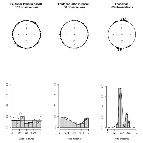
3.1 Feldspar Lath Orientations in Basalt
Feldspar crystals within rocks often align in parallel or subparallel patterns, providing valuable insights into the processes of rock formation and historical geological events, such as volcanic eruptions. Dataset B2 from Fisher (1993) contains measurements of the long-axis orientations of 133 feldspar laths in basalt. Table 1 (columns 2 to 4) presents maximized log-likelihood, Bayesian Information Criterion (BIC), and Akaike Information Criterion (AIC) values for fitted NNTS axial models with parameter ranging from 0 to 13. Figure 1 (left plot) shows a circular dot plot and histogram of the dataset along with the best-fitted NNTS axial densities selected by BIC () and AIC (). A uniformity test by Fernández-Durán and Gregorio-Domínguez (2024), applied by doubling the axial angle, rejects the null hypothesis of uniformity implied by the BIC-selected model () in favor of the multimodal NNTS axial model chosen by AIC (), yielding a p-value of less than 0.01.
Dataset B5 from Fisher (1993) contains orientations of an additional 60 feldspar laths in basalt. Fisher emphasized the importance of testing uniformity and determining the number of modes in this dataset. Table 1 (columns 5 to 7) presents maximized log-likelihood, Akaike Information Criterion (AIC), and Bayesian Information Criterion (BIC) values for NNTS axial models with parameter ranging from 0 to 6. Figure 1 (center plot) shows the histogram along with the best-fitting BIC and AIC models, both of which correspond to a unimodal and symmetric density with =1. We conducted a likelihood ratio test comparing a symmetric NNTS model with against an asymmetric NNTS model with , depicted as a dashed line in Figure 1 (center plot). The resulting p-value was 0.6077, indicating insufficient evidence to reject the simpler symmetric model () in favor of the asymmetric alternative (). When comparing the symmetric and asymmetric NNTS axial models with () using a likelihood ratio test for symmetry, the null hypothesis of symmetry is rejected at a 5% significance level with a p-value equal to 0.0459.
Additionally, the uniformity test by Fernández-Durán and Gregorio-Domínguez (2024) produced a p-value between 0.01 and 0.05, leading to the rejection of the null hypothesis of uniformity at a 5% significance level when comparing the uniform density model () with the best AIC- and BIC-selected NNTS axial models with . Our results are consistent with those of Fisher (1993), supporting both the non-uniformity and unimodality of the dataset.
3.2 Face Cleat in a Coal Seam
Face cleats are longitudinal fractures that represent significant geological features within coal seams-structures composed of coal deposits embedded within layers of rock. Variations in the orientation of these fractures can indicate hazardous mining conditions, including the potential presence of gas. Dataset B22 from Fisher (1993) includes 63 median directions of face cleats measured at the Wallsend Borehole Colliery in New South Wales, Australia. The median directions were measured at intervals of 20 meters along the coal seam. Consequently, the dataset exhibits sequential ordering, implying that the observations may not be independent. Despite the presence of potential dependence structures within the dataset, we analyzed the data as if it were a random sample to facilitate a direct comparison with results presented by Arnold and SenGupta (2006).
Table 1 (columns 8 to 10) provides maximized log-likelihood, Akaike Information Criterion (AIC), and Bayesian Information Criterion (BIC) values for fitted NNTS axial models with parameter ranging from 0 to 7. Figure 1 (right plot) shows the histogram along with the best-fitting AIC and BIC models, both of which select . The selected NNTS model with displays two prominent modes within the observed range of data. This result contrasts with findings by Arnold and SenGupta (2006), who considered only unimodal densities for the same dataset.
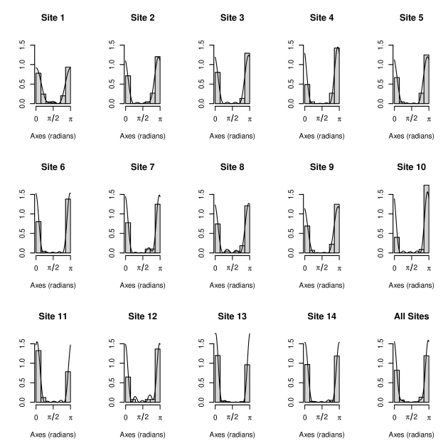
3.3 Orientations of Termite Mounds
Dataset B13 from Fisher (1993) contains measurements of termite mound orientations for the species Amitermes laurensis, collected from 14 sites on the Cape York Peninsula, North Queensland, Australia. Observed orientations were standardized to the interval between 0 and by subtracting from any measurement greater than . Figure 2 displays histograms for the orientation data at each of the 14 sites, along with sample sizes and geographical coordinates (latitude and longitude in degrees). The figure also shows the best-fitting NNTS axial densities according to the Bayesian Information Criterion (BIC) for each site. The final plot in Figure 2 presents the circular dot plot, histogram and the best BIC-fitted NNTS axial density for the combined data from all 14 sites, which serves as the basis for a likelihood ratio test of homogeneity, with the null hypothesis stating that the NNTS axial density is the same across all 14 sites. Table 2 provides maximized log-likelihood, AIC, and BIC values for NNTS axial densities with .
Applying a likelihood ratio test for homogeneity using the best-fitting BIC-selected NNTS models for the 14 individual sites compared to the best-fitting BIC NNTS model for the combined dataset yields a p-value of , assuming an asymptotic chi-squared distribution with 140 degrees of freedom. An alternative test, comparing the fitted NNTS models with at each site against a joint model, produces a p-value of 0.0062 with 130 degrees of freedom. In both tests, the null hypothesis of homogeneity across the 14 sites is rejected, indicating that variations exist in the orientation densities of termite mounds depending on their geographic location (latitude and longitude). These findings confirm the results obtained by Fisher (1993), who performed separate tests for the equality of mean directions and dispersions using a von Mises density model by doubling the axial angles to analyze them as circular data. However, it should be noted that the von Mises model is inherently unimodal and therefore unsuitable for modeling multimodal datasets, such as several of those shown in Figure 2, particularly evident in the histograms and fitted NNTS axial densities for site 8.
Fisher (1993) conducted tests of homogeneity specifically for pairs of sites 5 and 14, and sites 6 and 8. Using a von Mises density model by doubling the axial angles to analyze them as circular data, Fisher rejected the null hypothesis of equal mean directions for both pairs. However, for the pair of sites 6 and 8, Fisher concluded that the hypothesis of equal dispersions could not be rejected. To comprehensively compare our results with Fisher’s (1993) analysis, we performed likelihood ratio homogeneity tests for the same pairs (sites 5 and 14, and sites 6 and 8) using an NNTS axial model with parameter . The resulting p-values were 0.0051 for sites 5 and 14, and 0.0010 for sites 6 and 8, leading us to reject the null hypothesis of homogeneity for both pairs. These outcomes align with Fisher’s results, although Fisher’s tests separately evaluated mean directions and dispersions, while our approach employs a single integrated likelihood ratio test of overall homogeneity.
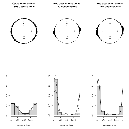
3.4 Magnetic Orientations of Ruminants
Using satellite imagery, deer bedding patterns in snow, and field observations, Begall et al. (2008) analyzed the body orientations of domestic cattle, red deer, and roe deer during grazing and resting, with respect to true (geographic) North, at various locations worldwide with differing magnetic declinations. Their analysis suggested that the primary factor influencing the animals’ orientations is alignment with Earth’s magnetic field, even after accounting for factors such as site-specific declination, wind direction, solar position, and temperature. For each of the three samples, Begall et al. (2008) clearly rejected the null hypothesis of uniformity using the Rayleigh uniformity test. We utilized the dataset from Begall et al. (2008), consisting of mean axial vector directions for herds observed at 308 locations for domestic cattle, 40 locations for red deer, and 201 locations for roe deer. Using these data, we fitted NNTS axial models and conducted homogeneity tests on the orientations across the three populations. Particular attention was paid to assessing homogeneity between red and roe deer populations.
Table 3 shows maximized log-likelihood, AIC, and BIC values for fitted NNTS axial models with different values of (from 0 to 5 for red deer, and from 0 to 10 for cattle and roe deer). When testing homogeneity across the three populations, we clearly rejected the null hypothesis, obtaining p-values of (best BIC model: for cattle, for red deer, for roe deer, and for all three populations combined) and (best AIC model: for cattle, for red deer, for roe deer, and for all three populations combined).
When testing homogeneity specifically between red deer and roe deer, we obtained p-values of 0.0511 (best BIC model with ) and 0.9999 (best AIC model with ). Figure 3 displays circular dot plots, histograms, and fitted density curves based on the best BIC and AIC NNTS axial models for cattle, red deer, and roe deer. For each population, the modes correspond to the average magnetic declination of the various sampling locations worldwide, as reported by Begall et al. (2008).
3.5 Leaf Inclination Angles
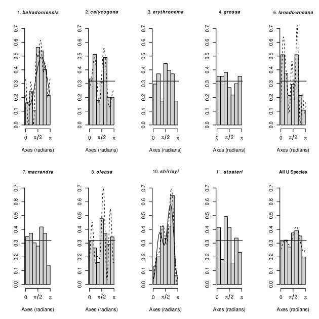
The spatial orientation of plant leaves, particularly leaf inclination angles, provides essential information regarding key biological processes such as photosynthesis efficiency, reflectance, temperature regulation, and overall resource utilization. Leaf inclination angle distributions vary according to plant species and geographic location. Recent advancements in digital imaging technology have significantly increased the availability of leaf inclination angle measurements, as algorithms can now efficiently determine these angles directly from digital images (see Pisek and Adamson, 2020).
In botanical studies, the leaf inclination angle typically ranges from 0 to . It is common practice in the literature to model the transformed linear variable using a Beta distribution with parameters and , and a probability density proportional to . Based on parameter estimates for different plant species, de Wit (1965) proposed six theoretical distributions for leaf orientation angles: planophile (leaves predominantly horizontal), erectophile (leaves predominantly vertical), plagiophile (leaves predominantly inclined), extremophile (leaves predominantly horizontal and vertical), spherical (leaves oriented isotropically like a sphere), and uniform. The parameters of the Beta distribution for the plagiophile case satisfy with , whereas for the extremophile case, they satisfy with , indicating that the Beta distribution takes equal values at the extremes 0 and 1 (see Chianucci et al., 2018). For the uniform distribution, the parameters satisfy . Therefore, the angle can be treated as an axial angle, and the distributions of for plants exhibiting plagiophile, extremophile, or uniform leaf distributions can be modeled using NNTS axial models.
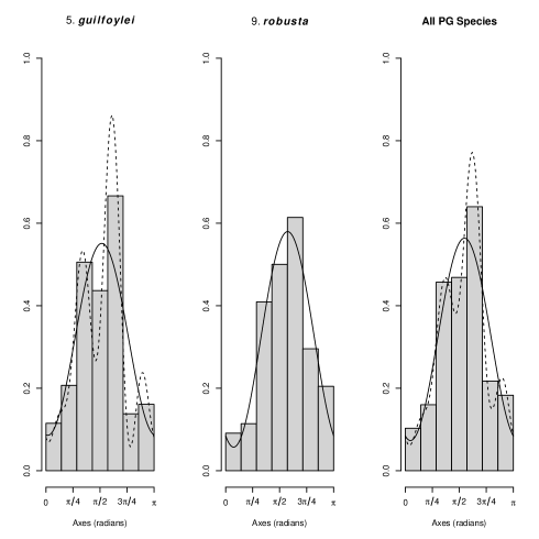
The dataset from Pisek and Adamson (2020) contains leaf inclination angle measurements for 71 species of gum trees (genus Eucalyptus). From these, we selected 11 species observed at the Huntington Library, Art Collections, and Botanical Gardens in Pasadena, California (latitude 34.125, longitude -118.114, altitude 207 m.a.s.l.), classified by Pisek and Adamson (2020) as either uniform (9 species) or plagiophile (2 species). Table 4 provides species names, sample sizes, Beta distribution parameter estimates, the optimal values for the best-fitting NNTS axial models based on the Bayesian Information Criterion (BIC), and the corresponding BIC values. Figures 4 and 5 display circular dot plots, histograms, and the best BIC-fitted NNTS axial densities for species classified as uniform (U) and plagiophile (PG), respectively.
Notably, for species classified as uniform (cases 1 balladoniensis and 10 shirleyi), neither the best BIC- nor AIC-selected NNTS axial densities corresponded to a uniform distribution (Figure 4). This observation is further confirmed by the uniformity test of Fernández-Durán and Gregorio-Domínguez (2024) shown in Table 4, where the null hypothesis of uniformity is rejected for cases 1 and 10 when comparing against either a NNTS axial model with or the best BIC-selected NNTS axial model. Moreover, when using the best AIC-selected NNTS axial model as an alternative, the hypothesis of uniformity is additionally rejected for cases 2, 6, and 8 at a 5% significance level.
4 Conclusions
A flexible new family of axial data densities is developed by identifying conditions under which NNTS densities, originally defined for circular data, are suitable for axial data. These NNTS axial densities may be uniform, symmetric, asymmetric, or multimodal, depending on parameter constraints. Efficient numerical optimization on manifolds, adapted from Fernández-Durán and Gregorio-Domínguez (2010), facilitates maximum likelihood estimation and enables direct implementation of likelihood ratio tests. The proposed methodology was successfully applied to real datasets involving the orientations of rocks, animals, and plants, showing excellent performance. Importantly, these results demonstrate significant improvements over previous methodologies that did not consider multimodal axial densities.
Acknowledgments
The authors wish to thank the Asociación Mexicana de Cultura, A.C. for its support and Prof. Sabine Begall for providing the dataset on magnetic orientations of ruminants.
References
- [1] Abe, T. Shimizu, K., Kuuluvainen, T. and Aakala, T. (2012). Sine-Skewed Axial Distributions with An Application Application to Fallen Tree Data. Environmental and Ecological Statistics, 19, 295-307.
- [2] Arnold, B.C. and SenGupta, A. (2006). Probability Distributions and Statistical Inference for Axial Data. Environmental and Ecological Statistics, 13, 271-285.
- [3] Arnold, B.C. and SenGupta, A. (2011). Models for Axial Data. In: Wells, M., SenGupta, A. (eds) Advances in Directional and Linear Statistics. Physica-Verlag HD.
- [4] Begall, S., Červený, J., Neef, J., Vojtěch, O. and Burda, H. (2008). Magnetic Alignment in Grazing and Resting Cattle and Deer, Proceedings of the National Academy of Sciences, 105, 13451-13455.
- [5] Chianucci, F., Pisek, J., Raabe, K., Marchino, L., Ferrara, C. and Corona, P. (2018). A Dataset of Leaf Inclination Angles for Temperate and Boreal Broadleaf Woody Species, Annals of Forest Science, 75:50.
- [6] de Wit, C.T. (1965). Photosyntesis of Leaf Canopies. Agricultural Research Report, no. 663, Wageningen.
- [7] Fernández-Durán, J.J. and Gregorio-Domínguez, M.M. (2010). Maximum Likelihood Estimation of Nonnegative Trigonometric Sums Models Using a Newton-like Algorithm on Manifolds. Electronic Journal of Statistics, 4, 1402-10.
- [8] Fernández-Durán, J.J. and Gregorio-Domínguez, M.M. (2012). CircNNTSR: An R Package for the Statistical Analysis of Circular Data Using Nonnegative Trigonometric Sums (NNTS) Models. R package version 2.0. http://CRAN.R-project.org/package=CircNNTSR
- [9] Fernández-Durán, J. J. and Gregorio-Domínguez, M. M. (2024). Sums of Independent Circular Random Variables and Maximum Likelihood Circular Uniformity Tests Based on Nonnegative Trigonometric Sums Distributions. AppliedMath, 4, 495-516. https://doi.org/10.3390/appliedmath4020026
- [10] Fisher, N.I. (1993). Statistical Analysis of Circular Data. Cambridge, New York: Cambridge University Press.
- [11] Mardia, K.V. and Jupp, P.E. (2000). Directional Statistics. Chichester, New York: John Wiley and Sons.
- [12] Pisek, J. and Adamson, K. (2020). Dataset of Leaf Inclination Angles for 71 Different Eucalyptus Species. Data in Brief, 33, 106391
- [13] R Development Core Team (2012). R: A language and environment for statistical computing. R Foundation for Statistical Computing, Vienna, Austria. ISBN 3-900051-07-0, URL http://www.R-project.org/.
| Feldspar laths in basalt | Feldspar laths in basalt | Face cleat | |||||||
|---|---|---|---|---|---|---|---|---|---|
| 133 observations | 60 observations | 63 observations | |||||||
| loglik | BIC | AIC | loglik | BIC | AIC | loglik | BIC | AIC | |
| 0 | -152.25 | 304.50* | 304.50 | -110.27 | 220.55 | 220.55 | -72.12 | 144.24 | 144.24 |
| 1 | -150.36 | 310.49 | 304.71 | -65.12 | 138.42* | 134.23* | -34.78 | 77.85 | 73.57 |
| 2 | -147.66 | 314.89 | 303.33 | -64.62 | 145.61 | 137.24 | -19.80 | 56.17 | 47.60 |
| 3 | -143.33 | 316.01 | 298.66 | -64.58 | 153.72 | 141.16 | -15.31 | 55.47 | 42.61 |
| 4 | -137.26 | 313.64 | 290.51* | -63.59 | 159.93 | 143.17 | -8.71 | 50.56 | 33.42 |
| 5 | -136.90 | 322.70 | 293.80 | -62.95 | 166.84 | 145.90 | 3.49 | 34.45 | 13.01 |
| 6 | -136.61 | 331.90 | 297.21 | -61.54 | 172.22 | 147.08 | 10.10 | 29.52* | 3.80* |
| 7 | -134.28 | 337.03 | 296.56 | 11.95 | 34.11 | 4.10 | |||
| 8 | -132.50 | 343.25 | 297.00 | ||||||
| 9 | -132.13 | 352.29 | 300.27 | ||||||
| 10 | -130.35 | 358.50 | 300.70 | ||||||
| 11 | -129.24 | 366.08 | 302.49 | ||||||
| 12 | -128.94 | 375.25 | 305.88 | ||||||
| 13 | -128.41 | 383.97 | 308.82 | ||||||
| Site | Latitude | Longitude | BIC | AIC | loglik | loglik 5 | |||
|---|---|---|---|---|---|---|---|---|---|
| 1 | 100 | -15∘ 43′′ | 144∘ 42′′ | 2 | 122.12 | 2 | 111.69 | -51.85 | -50.10 |
| 2 | 50 | -15∘ 32′′ | 144∘ 17′′ | 3 | 42.48 | 4 | 30.50 | -9.50 | -6.92 |
| 3 | 50 | -14∘ 59′′ | 143∘ 35′′ | 3 | 30.02 | 4 | 17.40 | -3.27 | -0.17 |
| 4 | 50 | -14∘ 19′′ | 143∘ 19′′ | 4 | 33.12 | 4 | 17.82 | -0.91 | 0.15 |
| 5 | 50 | -13∘ 21′′ | 142∘ 53′′ | 3 | 37.56 | 3 | 26.09 | -7.04 | -3.69 |
| 6 | 50 | -12∘ 50′′ | 142∘ 44′′ | 4 | 17.96 | 6 | 2.52 | 6.67 | 8.74 |
| 7 | 66 | -11∘ 54′′ | 142∘ 30′′ | 4 | 46.92 | 4 | 29.40 | -6.70 | -5.69 |
| 8 | 48 | -12∘ 06′′ | 142∘ 33′′ | 3 | 38.75 | 3 | 27.52 | -7.76 | -4.63 |
| 9 | 100 | -12∘ 29′′ | 142∘ 39′′ | 3 | 66.85 | 3 | 51.22 | -19.61 | -17.65 |
| 10 | 50 | -13∘ 12′′ | 142∘ 46′′ | 4 | 6.74 | 7 | -13.26 | 12.28 | 16.13 |
| 11 | 37 | -15∘ 02′′ | 143∘ 41′′ | 4 | 13.37 | 6 | -2.14 | 7.76 | 10.38 |
| 12 | 31 | -14∘ 47′′ | 143∘ 30′′ | 4 | 28.27 | 5 | 15.49 | -0.40 | 2.26 |
| 13 | 132 | -13∘ 50′′ | 143∘ 12′′ | 5 | -4.02 | 6 | -33.02 | 26.42 | 26.42 |
| 14 | 92 | -13∘ 50′′ | 143∘ 12′′ | 4 | 25.36 | 5 | 2.98 | 5.41 | 8.51 |
| all | 906 | 5 | 274.43 | 6 | 225.31 | -103.17 | -103.17 |
| Cattle | Red Deer | Roe Deer | Cattle, Red, Roe Deer | Red, Roe Deer | |||||||||||
|---|---|---|---|---|---|---|---|---|---|---|---|---|---|---|---|
| loglik | BIC | AIC | loglik | BIC | AIC | loglik | BIC | AIC | loglik | BIC | AIC | loglik | BIC | AIC | |
| 0 | -352.58 | 705.15 | 705.15 | -45.79 | 91.58 | 91.58 | -230.09 | 460.18 | 460.18 | -628.46 | 1256.91 | 1256.91 | -275.88 | 551.76 | 551.76 |
| 1 | -275.77 | 562.99* | 555.53 | -21.46 | 50.31 | 46.93 | -123.40 | 257.40 | 250.79 | -424.91 | 862.43 | 853.81 | -145.37 | 301.71 | 294.74 |
| 2 | -272.92 | 568.76 | 553.84* | -10.40 | 35.56 | 28.80 | -70.66 | 162.53 | 149.31 | -380.34 | 785.92 | 768.69 | -81.44 | 184.82 | 170.88 |
| 3 | -271.25 | 576.88 | 554.50 | -2.41 | 26.96* | 16.82 | -42.29 | 116.40 | 96.58 | -370.96 | 779.77 | 753.92 | -45.68 | 124.28 | 103.37 |
| 4 | -270.30 | 586.43 | 556.59 | 0.88 | 27.74 | 14.23 | -32.23 | 106.88 | 80.45 | -361.87 | 774.20* | 739.74 | -34.13 | 112.14 | 84.27 |
| 5 | -268.71 | 594.73 | 557.43 | 4.25 | 28.38 | 11.49* | -26.76 | 106.56 | 73.53 | -356.94 | 776.95 | 733.87* | -25.57 | 105.99 | 71.14 |
| 6 | -268.09 | 604.94 | 560.18 | -18.43 | 100.50* | 60.86* | -355.46 | 786.62 | 734.92 | -14.58 | 94.97* | 53.15* | |||
| 7 | -267.85 | 615.92 | 563.70 | -17.87 | 109.99 | 63.75 | -354.64 | 797.59 | 737.28 | -13.60 | 103.99 | 55.21 | |||
| 8 | -267.77 | 627.22 | 567.54 | -17.50 | 119.86 | 67.00 | -354.02 | 808.96 | 740.03 | -13.00 | 113.75 | 58.00 | |||
| 9 | -266.00 | 635.15 | 568.01 | -15.44 | 126.34 | 66.88 | -352.15 | 817.85 | 740.31 | -10.70 | 120.13 | 57.40 | |||
| 10 | -265.66 | 645.91 | 571.31 | -14.87 | 135.81 | 69.75 | -351.43 | 829.02 | 742.86 | -9.94 | 129.58 | 59.88 | |||
| id | Species name | Beta dist. | Type | p-value unif. test vs. | loglik | |||||||
| Eucalyptus … | =1 | |||||||||||
| 1 | balladoniensis | 83 | 1.62 | 1.31 | U | 1 | 5 | <0.01 | <0.01 | <0.01 | -87.59 | -77.71 |
| 2 | calycogona | 100 | 1.06 | 1.29 | U | 0 | 3 | <0.01 | >0.10 | -114.47 | -105.64 | |
| 3 | erythronema | 90 | 1.18 | 1.23 | U | 0 | 0 | >0.10 | -103.03 | -103.03 | ||
| 4 | grossa | 82 | 0.81 | 0.85 | U | 0 | 0 | >0.10 | -93.87 | -93.87 | ||
| 6 | lansdowneana | 83 | 0.96 | 1.29 | U | 0 | 5 | <0.01 | >0.10 | -95.01 | -79.00 | |
| 7 | macrandra | 96 | 1.04 | 1.20 | U | 0 | 0 | >0.10 | -109.89 | -109.89 | ||
| 8 | oleosa | 84 | 1.07 | 1.01 | U | 0 | 4 | >0.01 | >0.10 | -96.16 | -86.58 | |
| <0.05 | ||||||||||||
| 10 | shirleyi | 100 | 1.90 | 1.61 | U | 2 | 3 | <0.01 | <0.01 | <0.01 | -100.39 | -96.85 |
| 11 | stoateri | 86 | 1.02 | 1.15 | U | 0 | 0 | >0.10 | -98.45 | -98.45 | ||
| All U Species | 804 | 0 | 2 | <0.01 | <0.01 | -920.36 | -909.67 | |||||
| 5 | guilfoylei | 97 | 2.29 | 2.19 | PG | 1 | 4 | <0.01 | <0.01 | <0.01 | -95.95 | -87.69 |
| 9 | robusta | 98 | 2.64 | 2.13 | PG | 1 | 1 | <0.01 | <0.01 | <0.01 | -93.24 | -93.24 |
| All PG Species | 195 | 1 | 4 | <0.01 | <0.01 | <0.01 | -190.51 | -183.90 | ||||