Multimodal Techniques for Malware Classification
Abstract
The threat of malware is a serious concern for computer networks and systems, highlighting the need for accurate classification techniques. In this research, we experiment with multimodal machine learning approaches for malware classification, based on the structured nature of the Windows Portable Executable (PE) file format. Specifically, we train Support Vector Machine (SVM), Long Short-Term Memory (LSTM), and Convolutional Neural Network (CNN) models on features extracted from PE headers, we train these same models on features extracted from the other sections of PE files, and train each model on features extracted from the entire PE file. We then train SVM models on each of the nine header-sections combinations of these baseline models, using the output layer probabilities of the component models as feature vectors. We compare the baseline cases to these multimodal combinations. In our experiments, we find that the best of the multimodal models outperforms the best of the baseline cases, indicating that it can be advantageous to train separate models on distinct parts of Windows PE files.
1 Introduction
Rapid development in technology has changed the way humans use and acquire knowledge and interact with society, leading to an increased reliance on personal computers and smart devices. In recent decades, valuable information has become available on the Internet and on personal computers, and such data is a natural target for cybercriminals [1]. Cybercrime and malware go hand-in-hand, and hence malware detection and classification are vital concerns in cybersecurity.
Windows Portable Executable (PE) files are the most common victims of malware attacks. Due to their popularity, malware creators often choose to attack PE file formats [21].
Traditional signature-based detection methods are fast, efficient, and accurate for known threats. However, due to their dependency on predefined patterns or signatures of known malware, they lack adaptability and are vulnerable to evasion techniques. Malware that can change its code structure while maintaining malicious functionality can easily escape from the signature-based antivirus scanning [12]. As a result, machine learning and deep learning techniques have become mainstays in the malware detection field.
In this research, we apply machine learning techniques to the problem of Windows PE malware classification using a multimodal approach. In this context, multimodal means that we apply machine learning techniques that combine multiple types of data, with the goal of improving the accuracy of the system. Specifically, in this paper, we train learning models on different parts of PE files, then train another machine learning model with the probability vectors of the component models serving as features. While copious previous research has trained trained a wide variety learning models on a wide range of features, (byte sequences, opcode sequences, API calls, various graph structures, features derived from code analysis, metadata, and so on, there is relatively little research that attempts to directly utilize the structure inherent in PE files [24, 39, 44].
This research expands upon traditional methods by focusing on the structural characteristics of PE files, which are composed of headers and various additional sections (heretofore referred to simply as sections) . We extract features from PE headers and from the PE sections. Then we train models just using the header-based features, we train models just using the sections-based features, and we train models using features from both the header and sections (i.e., the entire PE file). We then train multimodal learning models using the output of the header and section models as the feature vectors. In this context, the output of a model refers to the probability vector generated by the output layer of the model. We then compare the results of these different cases, namely header-based models, section-based models, models trained on the entire PE file, and multimodal models trained on the output of header and sections based models. Note that in the multimodal cases, the training of the header based model and the sections based model can be viewed as a feature engineering step, with the output of these models yielding additional features that may be more informative, as compared to the original features used to train the component models.
For the header-based, sections-based models, and the models trained on the entire PE file, we experiment with Support Vector Machines (SVM), Long Short-Term Memory (LSTM) models, and Convolutional Neural Networks (CNN). For the multimodal models we use SVMs to combine the output of the header-based and sections-based models.
The remainder of this paper is organized as follows. Section 2 introduces relevant background topics, including an overview of the PE file format and the learning models employed in our experiments. In Section 3 we discuss representative examples of relevant related work. Section 4 presents our experiment, including dataset preparation, feature extraction, model design, hyperparameter tuning, and so on. In this section, we also compare and analyze our results. Section 5 summarizes the key findings of this research and provides some suggestions for further work.
2 Background
The Portable Executable (PE) file format is the standard for Windows executables. Due to their ubiquity, PE files are the predominant target for malware creators. According to a 2020 report from Kaspersky, nearly 90% of all malware detected daily occurred in PE files [20]. Given the frequency of this format in malware attacks, understanding the structure and functionality of PE files may be advantageous for malware analysis. Furthermore, a deep understanding of PE file structure facilitates the extraction of useful features for machine learning-based malware detection. Next, we provide an overview of the PE file format, which is followed by an introduction to the three types of machine learning models considered in this research.
2.1 Overview of the PE File Format
The PE file format is derived from the Microsoft Common Object File Format (COFF). It is a highly modular and structured file format that ensures portability and compatibility on various Windows platforms [5]. Compared to a single contiguous memory-mapped file, PE files utilize header information that provides detailed instructions to the Windows dynamic linker, enabling it to load code (including required libraries) into designated memory locations with the appropriate permissions. This approach is designed to ensure performance and safety during execution. Common PE format executable extensions include .exe, .dll, .scr, and .sys. While all of these file types adhere to the PE structure, each type include unique metadata or characteristics to support their specific use cases [10].
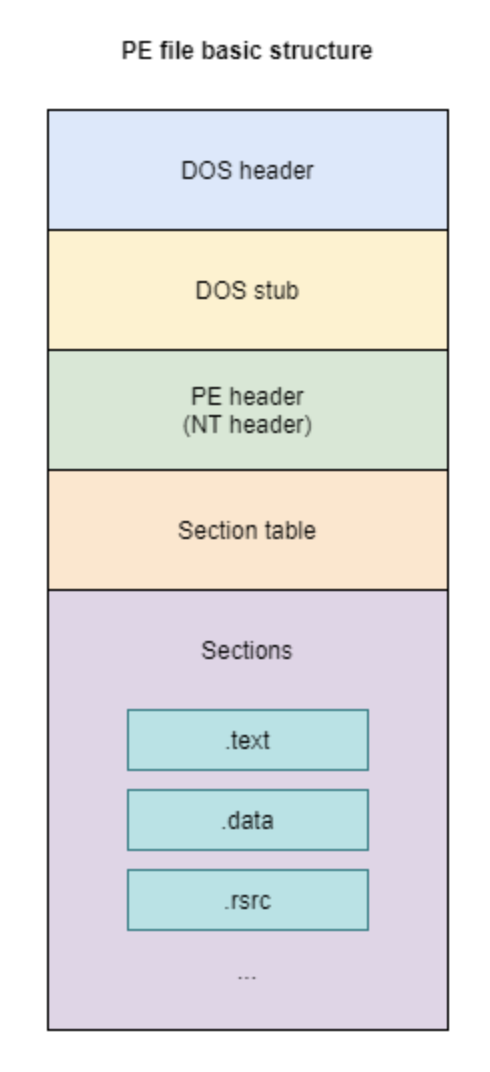
An example layout of the Windows PE file is shown in Figure 1. Note that the PE file includes the DOS Header, DOS Stub, PE File Header (aka NT header), Section Table, and Sections. Next, we briefly discuss each of these components of a PE file.
- DOS Header
-
— The DOS Header is the first data structure in a PE file. It provides backward compatibility with MS-DOS applications, which were applications designed to run in the Microsoft Disk Operating System (MS-DOS) environment during the beginning of 1980. The DOS Header occupies the first 64 bytes of the file, followed by a DOS stub program that outputs a message "This program cannot be run in DOS mode". This message is used to notify the users that the file is currently executing in a DOS environment. The first and last elements of the DOS Header are e_magic and e_lfanew, respectively. This first element, e_magic, is the two-byte “magic number” 0x5A4D (or MZ in ASCII), which is used to simply denote the file as an MS-DOS executable. The last member of the DOS Header structure, e_lfanew, is the offset to the NT headers. This field is crucial for the PE loader on Windows systems to determine where to locate the NT headers to begin loading the executable. An example of a DOS header is illustrated in Figure 2.
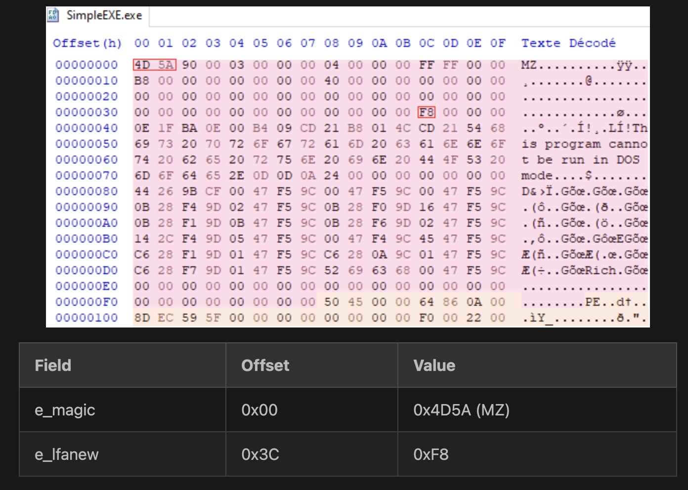
Figure 2: DOS header [38] - PE Header
-
— The PE Header (or NT header) begins with the PE signature (PE\0\0). It is a marker that identifies the file as a Portable Executable. It is followed by the COFF file header that provides metadata about the file, such as the target machine architecture, the number of sections, the file creation timestamp, and attributes that describe the file’s characteristics [5].
- Optional Header
-
— Contrary to its name, the Optional Header is not optional, as it is required for all PE image files. It provides necessary information like entry point address, the preferred memory location for loading, the size of the image in memory, and various attributes like subsystem type and security features. This header helps to guide the Windows loader in correctly loading and executing the program. However, it is optional for files like object files, which do not require runtime information [5].
- Section Table
-
— The Section Table is a series of section headers. Each entry in the table provides information for a specific section of the file, including the section name, virtual size, virtual address, raw data size, and assigned permissions. These headers contain the crucial information required by the loader to correctly map each section into memory with appropriate attributes, such as read, write, or execute permissions. Both the Section Table and the Optional Header play important roles in the loading and execution of a PE file but address different levels of detail: the Section Table focuses on sections, while the Optional Header provides a high-level view of the entire file and execution requirements.
- Sections
-
— The Sections represent the actual contents of the PE file, including executable code, initialized and uninitialized data, and various embedded resources. Common sections typically found in most PE files include the following.
- .text:
-
The .text section contains the executable instructions for the application. Within this section, the entry point can be found. In this research, it served as the starting point for section-based feature extraction. Notably, An application may include multiple sections containing executable instructions.
- .data:
-
The .data section holds initialized data, such as global and static variables. It often includes constants and strings defined in the source code.
- .rdata or .idata:
-
The .radata or .idata sections generally store read-only data and the import table. The import table lists the Windows API functions used by the executable file, along with the names of their associated dynamic link libraries. This information allows the Windows loader to locate and link the required API functions from the appropriate system dynamic link libraries.
- .reloc:
-
The .reloc session contains the relocation table, which provides information needed when the executable is loaded at a base address different from the one initially specified. It helps adjust the addresses of code and data references accordingly. By default, most executable files assume a preferred base address. It will be the starting address in memory where they expect to be loaded. If the program is loaded at the preferred base address, then all its hard-coded addresses will be correct, and the program can run without modification. However, if the executable is loaded to a different base address, this section would provide the necessary information.
- .rsrc:
-
The .rsrc section contains various embedded resources used by the executable, such as icons, dialogs, images, menus, and version information. These resources are typically part of the application’s user interface.
- .debug:
-
This .debug section stores debugging information, including symbols and source line references. It is used by debuggers to provide meaningful diagnostics during development.
2.2 Machine Learning Methods
This section introduces the machine learning that are used in the experiments considered in this paper. Specifically, we discuss Support Vector Machines (SVM), Long Short-Term Memory (LSTM) models, and Convolutional Neural Networks (CNN).
2.2.1 Support Vector Machines
The main ideas behind SVMs are the following.
-
•
Separating hyperplane — The goal is to separate labeled training data into two classes based on a hyperplane.
-
•
Maximize the margin — When constructing the separating hyperplane, we maximize the margin, which is defined as the minimum separation between the two classes in the training set.
-
•
Work in a higher dimensional space — By moving the problem to a higher dimension, there is more space available, and hence there is a better chance of finding a separating hyperplane.
-
•
Kernel trick — A kernel function can be used to transform the data to a higher dimensional space, with the goal of obtaining better separation. The reason that this is considered a “trick” is because we are able to work in a higher dimensional space, while paying a minimal performance penalty.
Figure 3 provides a generic view of linearly separable data, along with the separating hyperplane of an SVM, which maximizes the margin.
According to [4, p. 9], “SVMs are a rare example of a methodology where geometric intuition, elegant mathematics, theoretical guarantees, and practical algorithms meet.” We note in passing that the SVM technique easily generalizes to multiclass data, in which case the technique is sometimes referred to as Support Vector Classifier (SVC).
2.2.2 Long Short-Term Memory
In this section, we present long short-term memory (LSTM) networks in some detail. A vast number of variants of the LSTM architecture have been developed. However, according to an extensive empirical study [13], “none of the variants can improve upon the standard LSTM architecture significantly.”
In addition to being a tongue twister, LSTM networks are a class of RNN architectures that are designed to deal with long-range dependencies. That is, LSTM can deal with “gaps” between the appearance of a feature and the point at which it is used by the model [13]. The claim to fame of LSTM is that it can mitigate the effect of vanishing gradients, which is what enables such models to account for longer-range dependencies [16].
Before outlining the ideas behind LSTM, we note that the LSTM architecture has been one of the most commercially successful learning techniques ever developed. Among many other applications, LSTMs have been used in Google Allo [23], Google Translate [42], Apple’s Siri [25], and Amazon Alexa [15]. However, the commercial dominance of LSTM may be waning [29].
Figure 4 illustrates a generic LSTM. From this high level perspective, an obvious difference from a plain vanilla RNN is that an LSTM has two “lines” entering and exiting each state. As in a standard RNN, one of these lines represents the hidden state, while the second line is designed to serve as a gradient “highway” during backpropagation. In this way, the gradient can “flow” much further back with less chance that it will vanish along the way.
In Figure 5 we expand one LSTM cell that appears in Figure 4. Here, is the sigmoid function, is the hyperbolic tangent (i.e., ) function, the operators “” and “” are pointwise multiplication and addition, respectively, while “” indicates concatenation of vectors. The vector is the “input gate,” is the “forget gate,” and is the “output gate.” The vector is an intermediate gate and is sometimes referred to as the “gate gate” [26]. We have much more to say about these gates below.
The gate vectors that appear in Figure 5 are computed as
where the terms are biases. The outputs are given by
where, as mentioned above, “” is pointwise multiplication and “” is the usual pointwise addition. Note that each of the weight matrices is .
In matrix form, ignoring the bias terms, we have
where and are column vectors of length , and is a weight matrix of the form
Each of the gates , , , and is a column vector of length . Recall that the sigmoid squashes its input to be within the range of 0 to 1, whereas the function produces output within the range of to .
To highlight the intuition behind LSTM, we follow a similar approach as that given in the excellent presentation at [26]. Specifically, we focus on the extreme cases, that is, we pretend that the output of each sigmoid is either 0 or 1, and each hyperbolic tangent is either or . Under this assumption, the forget gate is a vector of 0s and 1s, where the 0s tell us the elements of that the model will forget (i.e., set to 0) and the 1s indicate the elements that the model will remember (i.e., retain).
Again, assuming we only have the extreme cases, the input gate and gate gate together determine which elements of to increment or decrement. Specifically, when element of is 1 and element of is , we increment element of . On the other hand, if element of is 1 and element of is , then we decrement element of . This serves to emphasize or de-emphasize particular elements in the new-and-improved cell state .
Finally, the output gate determines which elements of the cell state will become part of the hidden state . Note that the hidden state is fed into the output layer of the LSTM. Also note that before the cell states are operated on by the output gate, the values are first squeezed down to be within the range of to by the function.
Of course, in general, the LSTM gates are not simply counters that increment or decrement. But, the intuition holds, that is, the gates keep track of incremental changes, thus allowing relevant information to “flow” over long distances via the cell state. In this way, an LSTM can mitigate the gradient issues that arise in plain vanilla RNNs.
2.2.3 Convolution Neural Network
Artificial Neural Networks typically use fully connected layers, where a neuron at one layer is connected to all neurons at the layers above and below. A fully connected layer can deal effectively with correlations between any elements within the training vectors. However, due to these fully connected layers, the number of weight that must be determined via training can be vast. In contrast, a Convolution Neural Network (CNN), is designed to deal with local structure, which results in a dramatic reduction in the number of weights that must be learned during training. Thus, a key benefit of CNNs is that convolutional layers can be trained far more efficiently than fully connected layers.
For images, most of the relevant structure (edges and gradients, for example) is local. Hence, CNNs would seem to be an ideal tool for image analysis. However, CNNs have performed well in a wide variety of other problem domains. In general, any problem for which there exists a data representation where local structure predominates is a candidate for a CNN. In addition to images, local structure is of primary importance in fields such as text analysis and speech recognition, for example.
A convolutional layer is illustrated in Figure 6. In this case, five filters are trained on an RGB color image. By initializing the filters with different values, they can potentially learn different features.
CNNs typically employ multiple convolutional layers. The first convolutional layer learns intuitive features, such as edges and gradients, while higher convolutional layers learn progressively more abstract features, which ultimately allows for discrimination between complex classes, such as “cat” and “dog”. Pooling layers are frequently employed between convolutional layers, which serve to reduce the dimensionality, while also playing a role in translation invariance. Various regularization techniques are used when training CNNs so as to mitigate issues related to overfitting. For example, cutout regularization forces the model to consider different parts of an image when training.
A detailed discussion of CNNs can be found at [19], while the paper [7] provides some interesting insights. For a more intuitive discussion of CNNs, see [18], and visual representations can be found at [11] For our purposes, it is important to note that image-based analysis has recently proven highly effective for malware classification and analysis [17, 31, 43].
3 Related Work
In this section, we review examples of related work where PE file features have been used for malware classification. But first we mention that, in general, features used for malware analysis can be considered static or dynamic [9]. Static features are those that can be obtained directly from the the malware file, whereas dynamic features require code execution or emulation. Examples of static features include byte histograms and opcode sequences, whereas API calls and various graph-based features typically must be collected in a dynamic mode. Dynamic features are generally more robust with respect to obfuscation techniques, while it is typically fare more efficient to collect static features. In the experiments reported in this paper, we only consider static features.
In [2], the EMBER dataset is introduced and analyzed. This dataset consists of a large set of static features extracted from 1.1 million PE files. The features include byte histograms, metadata in the header, and import table characteristics. The result from this study shows that machine learning techniques applied to these static features can distinguish between malware and benign with good accuracy.
Rezaei et al. [34] proposed a method focusing on using features from the PE header. They combined deep learning techniques and clustering techniques with 324 bytes of the header to train a malware classification model. The result of this model show good accuracy in malware classification, even when faced with obfuscation techniques. Similarly, Kattamuri et al. [22] developed the SOMLAP dataset, which includes 51,409 samples, and from each sample, they extract 108 PE header attributes. They first apply feature reduction techniques using swarm optimization algorithms, including Ant Colony Optimization (ACO), Cuckoo Search Optimization (CSO), and Grey Wolf Optimization (GWO), which is followed by traditional machine-learning techniques. This research claimed to achieve a high malware detection accuracy. The two papers discussed in this paragraph illustrate the potential effectiveness of using header-based features.
Raff et al. [32] proposed an end-to-end deep learning approach that avoids the need for manual feature selection. This approach feeds the entire byte sequence of PE files directly into a neural network, skipping typical feature engineering steps. This allows the network to independently learn meaningful feature patterns. This approach showed high accuracy on large-scale datasets with one downside being heavy computational time. In addition, the technique struggled with obfuscated malware.
Damodaran [9] evaluated static, dynamic, and hybrid feature sets using Hidden Markov Models (HMMs). This paper highlights the trade-offs between different feature selection strategies and serves as a useful reference for optimizing feature selection methods. Static features like opcode sequences were found to be almost as effective as dynamic features in most cases. Hybrid approaches, which combine static and dynamic features, introduced additional complexity and failed to outperform standard approaches.
Finally, Wen and Chow [40] proposed a malware detection model based on CNNs. In this research, variable-size binary fragments obtained from PE files are considered. The research simulated real-world scenarios where network packet size limitations result in incomplete file captures, aiming to demonstrate the ability to deal with such fragmented input. The dataset was derived from antivirus tools and included examples of zero-day malware. Even with these challenges, the model still performed relatively well.
Table 1 summarizes the related work discussed in this section. Taken as a whole, these studies demonstrate that a wide variety of PE-based feature selection and extraction methods have been used to build high-performing malware detection systems. Typical features include header fields, byte sequences, specific sections of the file, and even the full binary content analyzed using learning techniques. Together, these features enhance the performance of both traditional machine learning and modern deep learning models in malware classification.
Research Main results Anderson and Roth [2] Combining static features improved malware detection Rezaei, et al. [34] Header-based features more robust against obfuscation Kattamuri, et al. [22] High accuracy with swarm optimization on header features Raff, et al. [32] Achieved high accuracy using PE file byte sequences, but struggled with obfuscation Damodaran, et al. [9] Static features nearly as effective as dynamic features; hybrid approaches add complexity without consistent gain Wen and Chow [40] Good accuracy using CNN models on fragmented inputs and effective for zero-day malware scenario
Multimodal Machine Learning (MML) has developed as an innovative approach, utilizing diverse data modalities to enhance the performance of models. In [3], Barua et al., review key advancements and challenges in MML, including the current state of the field, and they provide insights into challenges and potential solutions, while also discussing several frameworks and trends. One significant finding in this paper is the growing trend toward deep learning approaches. These approaches have gained attention due to their ability to effectively process complex multimodal data, particularly in areas such as representation learning, fusion techniques, and alignment strategies. Several deep learning architectures are mentioned for their contributions to MML applications, including CNNs, Recurrent Neural Networks (RNN), and transformer-based architectures.
In another paper, Zhai et al. [45] proposed an online classification model for darknet traffic classification that integrates a CNN and a Bidirectional Gated Recurrent Unit (BiGRU) to extract spatial and temporal features from packet payloads. To enhance the overall representation of network traffic, the model incorporates flow-level abstract features processed by a Multilayer Perceptron (MLP). The authors state that this multimodal approach improves accuracy across multiple categories while reducing time and memory consumption by approximately 50%. The authors claim that compared to state-of-the-art traffic classification models, the proposed method demonstrates superior classification performance.
Further, in [37], Shobhit and Bera proposed a deep learning-based malware detection system with a unique architecture that combines image representations, text representations, and Generative Adversarial Networks (GANs). This so-called ModCGAN system architecture comprises several key components, including an Image Autoencoder, a Text Autoencoder, and a GAN. They utilized log files containing API call sequences to generate both image and text representations. These representations are fed into the respective autoencoders and combined into a single feature vector. This feature vector is then used for malware classification purposes. The results demonstrated that this multi-modal approach effectively captures the dynamic behavior of malware, resulting in improved malware detection accuracy compared to traditional single-modality methods.
Lastly, in [14], Guo et al. propose another innovative approach called Multimodal Dual-Embedding Networks (MDENet), which they use to detect malware with highly similar features. MDENet leverages malware features from different modalities, such as malware images (generated from numeric features of malware samples) and malware “sentences” (created by organizing tokenized malware features into sentence-like structures). MDENet achieves good accuracy in both classifying known malware and detecting new, unknown families. Its effectiveness is validated through experiments on the popular Mailing dataset and the MAL-100+ dataset. This study provides further evidence of the value of a multimodal approach in addressing challenging malware problems.
4 Experiments and Results
In this section, we present experimental results comparing the performance of various multimodal approaches to typical machine learning models. We train models using histograms, byte sequences, and bytes interpreted as 2-dimensional images, depending on the model under consideration. For each of the three model types discussed in Section 2.2, namely, SVM, LSTM, and CNN, we train a model on the header, we train another model on the sections, and we train a third model on the entire file. Then we consider multimodal experiments, where we train an SVM on the output of each of the nine combinations of header and section models. We evaluate all of our models based on accuracy, which is computed as
where we have , , , and .
But, before we discuss our experimental results, we provide details on the dataset and features utilized in the experiments.
4.1 Dataset
All the experiments presented in this study are based on malware samples from the Malicia dataset—specifically, release_malicia_1.0 dataset—which consists of malicious files in raw PE file format, along with metadata that includes the class label for each sample [28]. The dataset contains a large number of families, many of which have only a few samples, so we restrict our attention to the following five malware families.
- Cridex
-
is designed to steal banking credentials. In addition, after infecting a system, Cridex may integrate the compromised device into a botnet and exploit it for malicious activities, such as generating spam or executing Distributed Denial of Service (DDoS) attacks [8].
- Harebot
-
is classified as both a backdoor and a rootkit. It installs itself on Windows systems without the user’s consent, enabling attackers to gain unauthorized access to devices, networks, applications, and sensitive user information [46].
- SecurityShield
-
is malware disguised as antivirus software. It secretly monitors and collects information about a user’s activity while falsely reporting virus detections to coerce users into purchasing unnecessary software [36].
- Zbot
-
, also known as Zeus, is a Trojan that commonly spreads through spam emails, social media links, or drive-by downloads. It monitors infected systems to steal sensitive information such as banking credentials and passwords [41].
- ZeroAccess
-
is a Trojan horse equipped with an advanced rootkit, allowing it to conceal its presence, create hidden files, install backdoors, and download additional malware for various malicious purposes.
Figure 7 lists the number of samples that we consider from each of these malware families. Thus, the dataset for our experiments consists of 2114 samples and five classes, with a large imbalance between classes.
4.2 SVM Results
For the SVM model, we use byte histogram features. The raw byte sequences are extracted and interpreted as integer values ranging from 0 to 255. These integer values are then gathered into relative histograms, which yields a feature vector of length 256, where each element is between 0 and 1, and the sum of all 256 elements is 1, i.e., the vector satisfies the requirements of a discrete probability distribution. These histograms serve as the feature sets for our SVM classification models.
We use an 80-20 stratified split for training and testing and 5-fold cross-validation. To determine the hyperparameters, we perform a grid search on the values listed in Table 2, using the header features. Note that the values selected are in boldface in Table 2.
Hyperparameter Values tested Description {0.001, 0.01, 0.1, 1, 10} Regularization parameter {0.001, 0.01, 0.1, 1} Kernel coefficient kernel {poly, linear, rbf} Kernel type
In Figure 8, we observe that the SVM performs well when applied to histogram features. The best results are for a model is trained on only the sections, while the header model performs slightly worse and the entire file gives almost the same results as the sections model.
4.3 LSTM Results
Our LSTM models are trained on byte sequences. Since the PE header is typically 324 bytes, this is the sequence length used for our header model. For efficiency, when training the sections model and the “entire” PE file model, we experiment with lengths of 1000 and 2000 bytes.
The structure of the LSTM models is detailed in Table 3. Note that the only variation between the models is the input sequence length.
Hyperparameter Value Batch size 30 Epochs 10 Data used for validation 20% Input sequence length (bytes) 324 Number of LSTM units 64 Activation function (hidden layer) Sigmoid Number of dense units (output layer) 5 Activation function (output layer) Softmax Loss function Categorical cross-entropy Optimizer Adam
From Figure 9 we observe that the LSTM model performed reasonably well on when trained in the PE header, the other models yielded very poor results. The malware files under consideration are typically much larger than 2000 bytes, and hence better results might be obtainable using longer sequence lengths. However, LSTM models are computationally expensive to train for large sequence lengths, and we have already obtained strong results for the sections and entire file cases using SVM models.
4.4 CNN Results
For our CNN models, we convert the raw bytes into simple images as follows. For the header model, we generate a “byte image” from the first 256 bytes of the PE header as
where is the byte of the PE file. In an analogous manner we construct byte images of size for both the sections and entire file features, beginning at byte in the sections case, and beginning at byte for the entire file case. Note that in both of these latter two cases, we are considering precisely 1024 bytes. These byte images are then converted into grayscale images using the Python library Pillow [30]. The conversion process involves interpreting the binary data as a sequence of unsigned 8-bit integers, and each value corresponds to the intensity of the corresponding grayscale pixel, and the pixel intensity values are then assigned to the image using the putdata method.
We experimented with various CNN architectures. Details on the selected architecture are given in Table 4.
Layer (type) Output shape Number of parameters conv2d (Conv2D) (None, 30, 30, 32) 320 max_pooling2d (MaxPooling2D) (None, 15, 15, 32) 0 flatten (Flatten) (None, 7200) 0 dense_1 (Dense) (None, 128) 921,728 dense_2 (Dense) (None, 5) 645
Figure 10 shows that our CNN models perform well in all three cases, with images based on the first 1024 bytes of the entire file yielding the best accuracy. These results demonstrates the efficacy of image-based techniques in general—and CNNs in particular—in the realm of malware classification.
4.5 Multimodal Models
For our multimodal experiments, we test all combinations of one of our header-based models with one of our sections-based models. Since we trained models with header features and models with sections features for each of three distinct cases (SVM, LSTM, and CNN), we have a total of nine multimodal combinations.
To combine our models in a multimodal fashion, the output layer probabilities of the header-based model and the sections-based model are concatenated, and the resulting vector serves as the feature vector for an SVM classifier. Since each model is trained to distinguish between five classes, the feature vectors for the final SVM classifier are all of length 10.
We note in passing that for this multimodal approach, training the header-based model and the sections-based model can be viewed as feature engineering steps, since these component models take the raw features as input and produce new features for the final SVM classifier. We also note that this feature engineering step is straightforward for LSTM and CNN models, but an SVM does not directly generate probabilities. Therefore, for our header-based and sections-based SVM models, we set svm.SVC(probability=True) in scikit-learn, which introduces a post-training probability calculation step.
The results for all of our multimodal models are summarized in Figure A.1 of the Appendix. In these results, multimodal models are specified in the form
where is the model trained using header-based features, is the model trained using section-based features, and is the multimodal model that acts as the classifier, based on the output—in the form of vectors of probabilities—of the models and . Each subfigure represents the accuracy—given to two decimal places—achieved by different combinations of models. Note that Figures A.1(a) through (c) are sorted by the header model, while Figures A.1(d) through (f) give the same results, but sorted by the sections model. As mentioned above, in all cases, SVM is used as the multimodal classifier.
Figure 11 provides a comparison of the best multimodal model result to the best results obtained with each of the individual models, namely, SVM, LSTM, and CNN. The best of the multimodal models are
which achieve accuracies of 0.9929 and 0.9930, respectively. We observe that these best multimodal accuracies are about 1% better than the best of the individual models.
While a 1% improvement may not seem overly impressive at first glance, it is important to note that the second-best model had already attained more than 98% accuracy. Therefore, the results show that the number of samples misclassified by our best multimodal model is about half the number that were misclassified by the best of the individual models. Thus, we conclude that the multimodal approach to PE malware classification considered in this paper appears to have genuine merit.
5 Conclusion and Future Work
In this paper, we demonstrated the effectiveness of combining multiple machine-learning models in a multimodal sense can enhance malware classification accuracy. For our baseline cases, we trained SVM, LSTM, and CNN models on features extracted from the PE header, and on features extracted from the other sections of the PE file, and we also trained these same models on the overall PE file. We then generated multimodal models, where the output layer probabilities of a PE-header model and a PE-sections model were combined and used as feature vectors to train an SVM classifier. In this multimodal approach, we were able to take advantage of the unique strengths of specific learning techniques on different parts of the Windows PE file, which improved classification accuracy, as compared to the baseline cases.
There are many potential directions for improvements and extensions of the research presented in this paper. Testing the techniques considered in this paper on a larger, more diverse, and more challenging dataset would aid in more accurately quantifying the effectiveness of such a multimodal approach. We could also consider additional features, such as opcode sequences, API calls, and various graph structures, and we could employ advanced feature engineering techniques, such as Word2Vec [6]. In a similar vein, it has been demonstrated that the method used to generate images from raw data can affect the accuracy of CNN classifiers [35], and hence more sophisticated image-generation techniques should be considered. Experiments involving additional learning techniques would also be interesting—in particular, Graph Neural Networks have shown considerable promise in the malware domain [27], and such techniques are likely to provide unique strengths in a multimodal setting.
References
- [1] Mohammad Nasser Alenezi, Haneen Khalid Alabdulrazzaq, Abdullah Abdulhai Alshaher, and Mubarak Mohammad Alkharang. Evolution of malware threats and techniques: A review. International Journal of Communication Networks and Information Security, 12(3):326–337, 2020.
- [2] Hyrum S. Anderson and Phil Roth. EMBER: An open dataset for training static PE malware machine learning models. https://arxiv.org/abs/1804.04637, 2018.
- [3] Arnab Barua, Mobyen Uddin Ahmed, and Shahina Begum. A systematic literature review on multimodal machine learning: Applications, challenges, gaps and future directions. IEEE Access, 11:14804–14831, 2023.
- [4] Kristin P. Bennett and Colin Campbell. Support vector machines: Hype or hallelujah? SIGKDD Explorations, 2(2):1–13, 2000.
- [5] Karl Bridge et al. PE format. https://learn.microsoft.com/en-us/windows/win32/debug/pe-format.
- [6] Aniket Chandak, Wendy Lee, and Mark Stamp. A comparison of word2vec, hmm2vec, and pca2vec for malware classification. In Mark Stamp, Mamoun Alazab, and Andrii Shalaginov, editors, Malware Analysis Using Artificial Intelligence and Deep Learning, pages 287–320. Springer, 2021.
- [7] Daphne Cornelisse. An intuitive guide to convolutional neural networks. https://medium.freecodecamp.org/an-intuitive-guide-to-convolutional-neural-networks-260c2de0a050, 2018.
- [8] Cridex malware. Computer Hope. https://www.computerhope.com/jargon/c/cridex-malware.htm, 2017.
- [9] Anusha Damodaran, Fabio Di Troia, Corrado Aaron Visaggio, Thomas H. Austin, and Mark Stamp. A comparison of static, dynamic, and hybrid analysis for malware detection. Journal of Computer Virology and Hacking Techniques, 13(1):1–12, 2015.
- [10] Satyajit Daulaguphu. A comprehensive guide to PE structure, the layman’s way. https://tech-zealots.com/malware-analysis/pe-portable-executable-structure-malware-analysis-part-2/#:~:text=And%20PE%20file%20format%20is,scr%2C%20and%20.
- [11] Adit Deshpande. A beginner’s guide to understanding convolutional neural networks. https://adeshpande3.github.io/A-Beginner%27s-Guide-To-Understanding-Convolutional-Neural-Networks/, 2018.
- [12] Daniel Gibert. Machine learning for windows malware detection and classification: Methods, challenges, and ongoing research. In Dimitris Gritzalis, Kim-Kwang Raymond Choo, and Constantinos Patsakis, editors, Malware: Handbook of Prevention and Detection, pages 143–173. Springer, 2025.
- [13] Klaus Greff, Rupesh Kumar Srivastava, Jan Koutník, Bas R. Steunebrink, and Jürgen Schmidhuber. LSTM: A search space odyssey. IEEE Transactions on Neural Networks and Learning Systems, 28(10):2222–2232, 2017. https://arxiv.org/pdf/1503.04069.pdf.
- [14] Jingcai Guo, Yuanyuan Xu, Wenchao Xu, Yufeng Zhan, Yuxia Sun, and Song Guo. MDENet: Multi-modal dual-embedding networks for malware open-set recognition. https://arxiv.org/abs/2305.01245, 2023.
- [15] Arpit Gupta. Alexa blogs: How Alexa is learning to converse more naturally. https://developer.amazon.com/blogs/alexa/post/15bf7d2a-5e5c-4d43-90ae-c2596c9cc3a6/how-alexa-is-learning-to-converse-more-naturally, 2018.
- [16] Sepp Hochreiter and Jürgen Schmidhuber. Long short-term memory. Neural Computation, 9(8):1735–1780, 1997. http://www.bioinf.jku.at/publications/older/2604.pdf.
- [17] Mugdha Jain, William Andreopoulos, and Mark Stamp. Convolutional neural networks and extreme learning machines for malware classification. Journal of Computer Virology and Hacking Techniques, 16(3):229–244, 2020.
- [18] Ioannis Kalfas. Modeling visual neurons with convolutional neural networks. https://towardsdatascience.com/modeling-visual-neurons-with-convolutional-neural-networks-e9c01ddfdfa7, 2018.
- [19] Andrej Karpathy. Convolutional neural networks for visual recognition. http://cs231n.github.io/convolutional-networks/, 2018.
- [20] Kaspersky. The number of new malicious files detected every day increases by 5.2% to 360,000 in 2020. https://www.kaspersky.com/about/press-releases/the-number-of-new-malicious-files-detected-every-day-increases-by-52-to-360000-in-2020, 2020.
- [21] Sanjay Katkar. Virus Bulletin: Inside the PE file format. https://www.virusbulletin.com/virusbulletin/2006/06/inside-pe-file-format/, 2006.
- [22] Santosh Jhansi Kattamuri, Ravi Kiran Varma Penmatsa, Sujata Chakravarty, and Venkata Sai Pavan Madabathula. Swarm optimization and machine learning applied to pe malware detection towards cyber threat intelligence. Electronics, 12(2), 2023.
- [23] Pranav Khaitan. Google AI blog: Chat smarter with Allo. https://ai.googleblog.com/2016/05/chat-smarter-with-allo.html, 2016.
- [24] Hyunjong Lee, Sooin Kim, Dongheon Baek, Donghoon Kim, and Doosung Hwang. Robust IoT malware detection and classification using opcode category features on machine learning. IEEE Access, 11:18855–18867, 2023.
- [25] Steven Levy. The iBrain is here—and it’s already inside your phone. Wired. https://www.wired.com/2016/08/an-exclusive-look-at-how-ai-and-machine-learning-work-at-apple/, 2016.
- [26] Fei-Fei Li, Justin Johnson, and Serena Yeung. Lecture 10: Recurrent neural networks. http://cs231n.stanford.edu/slides/2017/cs231n_2017_lecture10.pdf, 2017.
- [27] Vrinda Malhotra, Katerina Potika, and Mark Stamp. A comparison of graph neural networks for malware classification. Journal of Computer Virology and Hacking Techniques, 20:53–69, 2024.
- [28] Antonio Nappa, M. Zubair Rafique, and Juan Caballero. The MALICIA dataset: Identification and analysis of drive-by download operations. International Journal of Information Security, 14(1):15–33, 2015.
- [29] George Philipp, Dawn Song, and Jaime G. Carbonell. The exploding gradient problem demystified — Definition, prevalence, impact, origin, tradeoffs, and solutions. https://arxiv.org/pdf/1712.05577.pdf, 2018.
- [30] Pillow. https://pillow.readthedocs.io/en/stable/, 2011.
- [31] Pratikkumar Prajapati and Mark Stamp. An empirical analysis of image-based learning techniques for malware classification. In Mark Stamp, Mamoun Alazab, and Andrii Shalaginov, editors, Malware Analysis Using Artificial Intelligence and Deep Learning, pages 411–435. Springer, 2021.
- [32] Edward Raff, Jon Barker, Jared Sylvester, Robert Brandon, Bryan Catanzaro, and Charles K. Nicholas. Malware detection by eating a whole EXE. In The Workshops of the The Thirty-Second AAAI Conference on Artificial Intelligence, volume WS-18 of AAAI Technical Report, pages 268–276, 2018.
- [33] Reverse engineering portable executables PE — part 2. Mossé Cyber Security Institute. https://library.mosse-institute.com/articles/2022/05/reverse-engineering-portable-executables-pe-part-2/reverse-engineering-portable-executables-pe-part-2.html, 2022.
- [34] Tina Rezaei, Farnoush Manavi, and Ali Hamzeh. A PE header-based method for malware detection using clustering and deep embedding techniques. Journal of Information Security and Applications, 60:102876, 2021.
- [35] Nhien Rust-Nguyen, Shruti Sharma, and Mark Stamp. Darknet traffic classification and adversarial attacks using machine learning. Computers & Security, 127:103098, 2023. https://www.sciencedirect.com/science/article/pii/S0167404823000081.
- [36] SecurityShield. Microsoft Security Intelligence. https://www.microsoft.com/en-us/wdsi/threats/malware-encyclopedia-description?Name=SecurityShield, 2019.
- [37] Shobhit and Padmalochan Bera. ModCGAN: A multimodal approach to detect new malware. In 2021 International Conference on Cyber Situational Awareness, Data Analytics and Assessment, CyberSA, pages 1–2, 2021.
- [38] Skr1x. Introduction to the PE file format. https://skr1x.github.io/portable-executable-format/, 2020.
- [39] Qiyu Wang. Support vector machine algorithm in machine learning. In 2022 IEEE International Conference on Artificial Intelligence and Computer Applications, ICAICA, pages 750–756, 2022.
- [40] Qiaokun Wen and K.P. Chow. CNN based zero-day malware detection using small binary segments. Forensic Science International: Digital Investigation, 38:301128, 2021.
- [41] Win32/Zbot. Microsoft Security Intelligence. https://www.microsoft.com/en-us/wdsi/threats/malware-encyclopedia-description?Name=Win32/Zbot, 2017.
- [42] Yonghui Wu et al. Google’s neural machine translation system: Bridging the gap between human and machine translation. https://arxiv.org/abs/1609.08144, 2016.
- [43] Sravani Yajamanam, Vikash Raja Samuel Selvin, Fabio Di Troia, and Mark Stamp. Deep learning versus gist descriptors for image-based malware classification. In Paolo Mori, Steven Furnell, and Olivier Camp, editors, Proceedings of the 4th International Conference on Information Systems Security and Privacy, ICISSP, pages 553–561, 2018.
- [44] Baoguo Yuan, Junfeng Wang, Dong Liu, Wen Guo, Peng Wu, and Xuhua Bao. Byte-level malware classification based on Markov images and deep learning. Computers & Security, 92:101740, 2020.
- [45] Jiangtao Zhai, Haoxiang Sun, Chengcheng Xu, and Wenqian Sun. ODTC: An online darknet traffic classification model based on multimodal self-attention chaotic mapping features. Electronic Research Archive, 31(8):5056–5082, 2023.
- [46] ZulaZuza. EnigmaSoft: Rootkit.HareBot. https://www.enigmasoftware.com/rootkitharebot-removal/, n.d.
Appendix
The results of all multimodal combinations tested are given in Figure A.1. For additional details on the multimodal experiments used to generate these results, see Section 4.5.
|
|
|
|
(a) SVM header models |
(b) LSTM header models |
|
|
|
|
(c) CNN header models |
(d) SVM sections models |
|
|
|
|
(e) LSTM sections models |
(f) CNN sections models |