Multiparameter quantum metrology using strongly interacting spin systems

Quantum metrology exploits quantum resources of well-controlled quantum systems to measure small signals with high sensitivity, and has great potential for both fundamental science and concrete applications [1, 2, 3, 4, 5, 6, 7, 8]. Interacting quantum systems have been recently recognized as an unprecedented playground to develop precise metrology [9, 10, 11, 12, 13, 14, 15, 16], where the interactions between probe systems can be a valuable quantum resource to improve the precision and other metrological performance, such as the achievement of metrological sensitivity beyond the Heisenberg limit [17, 18, 19, 20], the robustness against thermal noise [13], criticality-enhanced metrology [16, 21, 22, 23], and the evasion of rapid thermalization [24, 25, 11]. Moreover, the use of interactions that correlate probe systems can relax the experimental challenge of preparing entangled probe states [14, 26].

However, the current framework of interaction-based quantum metrology mainly focuses on single-parameter estimations [19, 13, 18, 14, 17, 15, 24, 16, 21, 20], neglecting many possible applications under realistic conditions. Indeed, numerous metrological applications are intrinsically multiparameter, such as measuring electric, magnetic, or gravitational fields. As a consequence, the field of multiparameter metrology has been intensively studied both theoretically and experimentally [27, 28, 29, 30, 31, 32, 33, 34, 35, 36]. The potential combination of interaction-based metrology and multiparameter estimation would open up exciting possibilities for developing precise metrology in applied and fundamental physics, such as quantum imaging [37, 38], sensor networks [39], navigation [40, 41, 42], the detection of vector fields [32, 33, 43, 34, 35], as well as the searches for spin-gravity coupling and ultralight dark matter axions [44, 45, 46]. Despite these appealing features, a demonstration of multiparameter metrology using the resource of interactions was heretofore lacking.

Here, we demonstrate an approach to interaction-based multiparameter estimation with the use of strongly interacting nuclear spins in molecules. We find that, as the interactions among nuclear spins become significantly larger than their Larmor frequencies, a different regime emerges where the strongly interacting spins can be simultaneously sensitive to all components of a multidimensional field, such as three-dimensional magnetic field and inertial rotation. Moreover, we observe that strong interactions between nuclear spins can increase their quantum coherence times as long as several seconds, leading to enhanced measurement precision. We experimentally illustrate the power of interaction-based multiparameter estimation by applying this approach to simultaneously estimating all three components of a magnetic field. Our work also provides a recipe for precisely measuring magnetic pseudo-fields originating from inertial rotation and constituting a new zero-field vector gyroscope. The present interaction-based metrology should be generic and promises to develop an entirely new class of multiparameter quantum sensors using a broad range of strongly interacting quantum systems, and will impact diverse metrological applications.

We would like to emphasize the difference of multiparameter metrology between this work and others. Although a variety of multiparameter quantum sensors have demonstrated the capability of measuring magnetic fields and inertial rotations [32, 33, 43, 34, 42, 35, 47, 36], they all make use of non-interacting probe systems, such as electron and nuclear spins. For example, all nuclear magnetic resonance (NMR) magnetometers tested so far use only a single spin species (for example, proton rich substances or noble gas ³He) that yields a single resonance line at the precession frequency [48, 49, 50]. Therefore, these magnetometers measure only the magnitude of the magnetic field, providing no information on its orientation. In conventional methods, external reference fields are additionally required to access the orientation information [32, 33, 34, 35]. This unavoidably produces significant static and radio frequency fields contamination, which are classical noise and would be a bottleneck for reaching the fundamental precision beyond the standard quantum limit. Unlike previous works, our work uses a different scheme in which strongly interacting spins are intrinsically sensitive to multidimensional fields. Thus, our work can avoid the classical noise caused by previously-required reference fields, thus opening a feasible route towards realizing multiparameter quantum sensors with quantum noise-limited sensitivity.

Nuclear and electron spin systems are progressively becoming a paradigm for precision metrology. Here nuclear-spin systems are used as a platform to develop multiparameter metrology. We focus on the estimation of all three components of an unknown magnetic field. In contrast to existing works based on non-interacting spins [32, 33, 43, 34, 42, 35], we employ a collection of molecules, where each molecule contains at least two different types of nuclear spins that interact with each other by an exchange interaction (a Heisenberg interaction). When such nuclear spins are imposed in a magnetic field $\mathbf{B}(\theta,\phi)$, they can be described by the Hamiltonian,

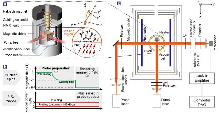
where $\gamma_{j}$ denotes the gyromagnetic ratio of the $j$th spin (here we set $\hbar=1$), $\mathbf{I}_{j}=(\hat{I}_{jx},\hat{I}_{jy},\hat{I}_{jz})$ is the spin angular momentum operator of the $j$th spin, $\mathbf{I}_{i}\cdot\mathbf{I}_{j}$ is called a Heisenberg interaction, and ${J_{ij}}$ is the strength of the Heisenberg interaction between the $i$th and $j$th spins. As shown in Fig. 1a, the unknown magnetic field $\mathbf{B}(\theta,\phi)=(B\sin\theta\cos\phi,B\sin\theta\sin\phi,B\cos\theta)$ is parameterized with the polar angle $\theta$, azimuthal angle $\phi$ and magnitude $B$, which are unknown parameters to be estimated.

Our interaction-based multiparameter estimation includes three stages: probe preparation, encoding with the strongly interacting spins, and probe readout, as shown in Fig. 1b. The initial probe state of nuclear spins is prepared as $\rho_{0}$, which is described in Appendix C1 for details. In the encoding stage, the key ingredient is the use of the quantum dynamics of the strongly interacting spins to encode the unknown parameters,

where $\rho(\theta,\phi,B,t)$ is the time-dependent density matrix of nuclear spins. Then, an atomic vapour sensor as a detector continuously measures the time-evolution of the nuclear magnetization $\textrm{Tr}[\rho(\theta,\phi,B,t)\hat{\mathbf{O}}_{z}]$ [51, 52, 53, 54]. Here, $\hat{\mathbf{O}}_{z}=\sum_{j}\gamma_{j}{\hat{I}}_{jz}$ represents the observable operator of $z$-magnetization. The observation values can be Fourier transformed into a spectrum. Consequently, the information of $\mathbf{B}(\theta,\phi)$ in the Hamiltonian $\mathcal{H}(\theta,\phi,B)$ can be encoded into the spectrum of the interacting spins, where each spectrally separating line corresponds to the transition between relevant eigenstates $|\Psi_{i}\rangle$ and $|\Psi_{j}\rangle$ of $\mathcal{H}(\theta,\phi,B)$ and its amplitude is proportional to a product of $\langle\Psi_{i}|\rho_{0}|\Psi_{j}\rangle\langle\Psi_{j}|\hat{\mathbf{O}}_{z}|\Psi_{i}\rangle$ [see Eqs. (11) and (12) in Appendix].

To show the explicit dependence on $\theta$ and $\phi$ of the spectral amplitudes, we introduce a convenient orthonormal coordinate system, where $\mathbf{z^{\prime}}=\mathbf{B}/B$, $\mathbf{x^{\prime}}=\frac{\partial\mathbf{z^{\prime}}}{\partial\theta}$, and $\mathbf{y^{\prime}}=(\frac{1}{\sin\theta})\frac{\partial\mathbf{z^{\prime}}}{\partial\phi}$ (see Appendix C2 for details), as shown in Fig. 1a. Consequently, $\langle\Psi_{i}|\hat{\mathbf{O}}|\Psi_{j}\rangle=\mathcal{P}(\theta,\phi)\langle\Psi_{i}|\hat{\mathbf{O}^{\prime}}|\Psi_{j}\rangle$, where $\mathcal{P}(\theta,\phi)$, depending on $\theta$ and $\phi$, is a $3\times 3$ transformation matrix [see Eq. (15)] and $\hat{\mathbf{O}}^{\prime}_{l^{\prime}}=\sum_{j}\gamma_{j}\hat{I}_{jl^{\prime}}$ ($l^{\prime}=x^{\prime},y^{\prime},z^{\prime}$). Importantly, we note that the transition amplitudes in the new defined coordinates $\langle\Psi_{i}|\hat{\mathbf{O}}^{\prime}|\Psi_{j}\rangle$ are independent of the magnetic field orientation ($\theta,\phi$) [see Eq. (17)], where $\langle\Psi_{i}|\hat{\mathbf{O}}^{\prime}_{z^{\prime}}|\Psi_{j}\rangle$ and $\langle\Psi_{i}|\hat{\mathbf{O}}^{\prime}_{x^{\prime},y^{\prime}}|\Psi_{j}\rangle$ respectively correspond to the observation parallel or perpendicular to the magnetic field and hence the zero- or single-quantum resonance line. Thus, the observed amplitudes of zero- and single-quantum lines therefore can be used to estimate the multiple parameters of $\theta$, $\phi$ and $B$ [see Eq. (20) in Appendix], and in turn the magnetic field vector $\mathbf{B}(\theta,\phi)$.

We now explain why the strong interaction is a valuable resource for multiparameter estimation. The situation is considered where the Heisenberg interactions are much stronger than those Larmor frequencies ($|J|\gg|\gamma_{j}B|$); in this situation, the nuclear spins in each molecule strongly interact with each other. Strong interactions between spins can modify the energy level structure of the system, enabling the direct detection of some forbidden transitions that are pivotal for our multiparameter estimation. To show in more detail, we focus on two-spin case. The eigenstates of the two-spin system in an arbitrary magnetic field are $|\Psi_{1}\rangle=\mid\uparrow\uparrow\rangle$, $|\Psi_{2}\rangle=\cos\xi\mid\uparrow\downarrow\rangle+\sin\xi\mid\downarrow\uparrow\rangle$, $|\Psi_{3}\rangle=\cos\xi\mid\uparrow\downarrow\rangle$ $-\sin\xi\mid\downarrow\uparrow\rangle$, $|\Psi_{4}\rangle=\mid\downarrow\downarrow\rangle$ [55], where $\mid\uparrow\rangle$ and $\mid\downarrow\rangle$ are the eigenstates of spin operators $\hat{I}_{jz^{\prime}}$ along the quantization axis $z^{\prime}$ (defined by the direction of magnetic field, see Fig. 1a) and $\tan(2\xi)=\frac{J}{(\gamma_{1}-\gamma_{2})B}$. The transition between $|\Psi_{2}\rangle$ and $|\Psi_{3}\rangle$ corresponds to a zero-quantum transition, and the transition probability is $p=|\langle\Psi_{2}|\hat{\mathbf{O}}_{z^{\prime}}|\Psi_{3}\rangle|=1/2|(\gamma_{1}-\gamma_{2})\sin(2\xi)|$. We immediately see that the strong interacting regime ($|J|\gg|\gamma_{1}B|,|\gamma_{2}B|$) is of particular interest, since $|\Psi_{2}\rangle$ and $|\Psi_{3}\rangle$ are entangled states between two spins and their transition probability $p\rightarrow|\gamma_{1}-\gamma_{2}|/2$. For non-interacting ($J=0$) and weakly interacting ($|J|\ll|\gamma_{1}B|,|\gamma_{2}B|$) cases, $p\rightarrow 0$, so the zero-quantum line should never be detected directly. In contrast, strongly interacting spins can produce oscillating magnetization along the magnetic-field direction ($z^{\prime}$). In this situation, zero-quantum spectral lines are detectable and moreover they are very narrow lines due to long-lived coherence mechanism [56]. Based on these unforbidden transitions in strongly interacting spin systems that encode unknown parameters, multiparameter estimation becomes possible.

It is important to experimentally measure the transition lines of the strongly interacting nuclear spins under the measured magnetic field. We consider a star topology with one central nuclear spin, and $n$-1 equivalent spins in liquid-state molecules, such as ¹³CH_n molecules, as the testbed. A liquid of such molecules is contained in a glass tube with a 100-$\mu$L volume and polarized with a permanent magnet ($\approx 1.3$ T). Then the liquid is pneumatically shuttled to a sensing region $\sim 1$ mm above the atomic vapour cell (shown in the inset of Fig. 1a). During the shuttling, a guiding field ($\approx 10^{-4}$ T) is applied on the spins, allowing adiabatic transfer of the polarized nuclear spins into the sensing region and preserving the spin polarization [51, 52, 53, 54]. The nuclear-spin coherence times ($\tau_{\textrm{coh}}$) of the spin clusters are typically a few seconds (see Appendix A2). As a result, the spin polarization is initialized through controlling the direction of the guiding field [see Eq. (9) in Appendix]. After the guiding field is turned off within 10 $\mu$s, subsequent evolution of the spin state produces oscillating magnetization under the magnetic field to be estimated [see Eq. (11)]. The magnetization encodes the information about the magnetic field and is read out by an atomic vapour sensor (Fig. 1c, see Appendix for details).

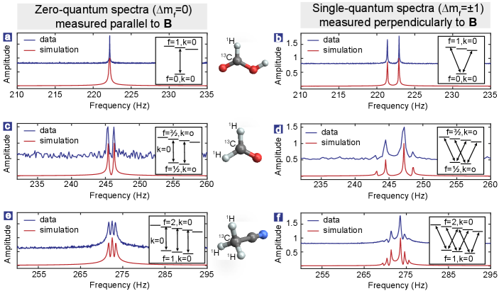
We first measure different quantum transitions of ¹³CH_n molecules. When one measures the spins along an axis parallel to the magnetic field $\mathbf{B}$ (i.e., $\theta=0$), the selection rules for allowed transitions are (referred as zero-quantum transitions): $\Delta f=0,\pm 1$, $\Delta m_{f}=0$. For example, formic acid yields a single resonance line at $222.2$ Hz (Fig. 2a). On the other hand, if one measures the spins along an axis perpendicular to the magnetic field $\mathbf{B}$ (i.e., $\theta=\pi/2$), the selection rules for allowed transitions are (referred as single-quantum transitions): $\Delta f=0,\pm 1$, $\Delta m_{f}=\pm 1$. In this case, formic acid yields two resonance lines centered at 222.2 Hz (Fig. 2b) split by $(\gamma_{h}+\gamma_{c})B$. Here, gyromagnetic ratios $\gamma_{c}\approx 10.7077$ MHz/T for carbon spins and $\gamma_{h}\approx 42.5775$ MHz/T for proton spins. Spectra of other ¹³CH_n molecules show similar patterns, as shown in Fig. 2c-f. The detailed splitting patterns are analysed in Eqs. (4)-(7) in Appendix B1. Additionally, zero- and single-quantum transitions can be simultaneously allowed when one measures the spins along an axis neither parallel nor perpendicular to the magnetic field. This implies that the information of magnetic-field orientation can be extracted from the observed spectral lines of ¹³CH_n molecules. Similar phenomena have been explored in the context of optical spectroscopy of multi-electron atoms [57, 58] but, to our knowledge, our work represents the first experimental demonstration in NMR spectroscopy.

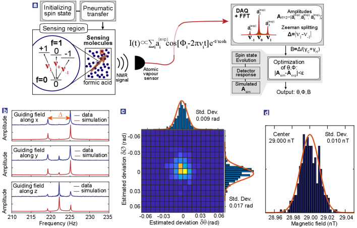
As a proof-of-principle demonstration, we use formic acid to estimate all three components of a magnetic field. As shown in Fig. 3a, in one single scan measurement, the amplitudes of three spectral lines at frequency $\nu_{0}$ for zero-quantum and at frequency $\nu_{\pm 1}$ for single-quantum are simultaneously recorded by the normalized form of $\mathbf{A}_{\textrm{exp}}=[\textrm{a}_{1}^{(\textrm{exp})}(\nu_{-1}),\textrm{a}_{2}^{(\textrm{exp})}(\nu_{0}),\textrm{a}_{3}^{(\textrm{exp})}(\nu_{1})]$. The magnetic field induces the Zeeman splitting $\Delta=|\nu_{1}-\nu_{-1}|$ of the doublet and, accordingly, the magnitude of the measured field can be determined in advance through $\Delta=(\gamma_{c}+\gamma_{h})B$ [the splittings $\Delta$ for arbitrary ¹³CH_n molecules are shown in Eqs. (4)-(7) in Appendix]. Furthermore, we use a model [see Appendix C] to calculate the amplitudes of relevant NMR lines, labelled by $\mathbf{A}_{\textrm{sim}}(\theta,\phi)=[\textrm{a}_{1}^{(\textrm{sim})}(\nu_{-1}),\textrm{a}_{2}^{(\textrm{sim})}(\nu_{0}),\textrm{a}_{3}^{(\textrm{sim})}(\nu_{1})]$ when $\theta$ and $\phi$ are given. Conversely, the parameters of $\theta$, $\phi$ can be obtained by minimizing the norm $|\mathbf{A}_{\textrm{sim}}(\theta,\phi)-\mathbf{A}_{\textrm{exp}}|$. However, multiple pairs of $(\theta,\phi)$ may result in the same spectrum if they satisfy certain symmetric conditions. To remove this ambiguity, we measure the nuclear-spin spectra and three sets of $\mathbf{A}_{\textrm{exp}}$ under various initial states $\rho_{0}$ by controlling the guiding field along ${x}$, ${y}$ and ${z}$ [51], in turn. The corresponding NMR spectra are shown in Fig. 3b. The $\theta,\phi$ can be unambiguously determined by finding the simulated $\mathbf{A}_{\textrm{sim}}(\theta,\phi)$ that simultaneously best matches the measured $\mathbf{A}_{\textrm{exp}}$ under three initial states. The magnetic field is determined to be such that $\theta\approx 1.289$ rad and $\phi\approx 0.047$ rad, and $B\approx 1.0788\cdot 10^{-7}$ T. The simulated Fourier spectra with red lines are in a good agreement with the experimental spectra.

In order to benchmark the precision of multiparameter estimation in our protocol, we simulate the performance of $\theta$, $\phi$ deviation under the influence of spectral amplitude variance. The variances $\{\delta\textrm{a}_{1}^{(\textrm{exp})},\delta\textrm{a}_{2}^{(\textrm{exp})},$ $\delta\textrm{a}_{3}^{(\textrm{exp})}\}$ are assumed to obey Gaussian noise $\sim\mathcal{N}(0,\sigma^{2})$, which comes mainly from the photon-shot noise of the probe beam in our experiment. Figure 3c shows the $\theta$, $\phi$ joint statistical distribution with $\sigma=0.01$ (corresponding to our current experimental signal-to-noise ratio (SNR) of 100). The uncertainties (standard deviations) of $\theta$, $\phi$ values are respectively estimated to be $\sigma_{\theta}\approx 0.009$ rad and $\sigma_{\phi}\approx 0.017$ rad, as shown in their histograms of deviations. One could increase, for example, the nuclear-spin initial polarization and NMR detector sensitivity, to decrease $\sigma$ and then achieve better orientation resolution.

We next discuss how precisely we can determine the magnitude of a magnetic field vector. The magnetic magnitude can be achieved by exploiting the Zeeman splitting of strongly interacting nuclear spins, for example, using the splitting $\Delta$ in the formic acid spectrum. For other ¹³CH_n molecules, there exists similar Zeeman splitting that can be used to measure the magnetic field magnitude [see Eqs. (4)-(7) in Appendix]. We use a set of such measurements to quantify the estimation precision. The uncertainties of $\Delta$ in the frequencies extracted from spectral profile fits are in the order of $0.3~{}\textrm{mHz}$. As shown in Fig. 3d, the statistical standard deviation of absolute magnetic field is $10^{-11}~{}\textrm{T}$.

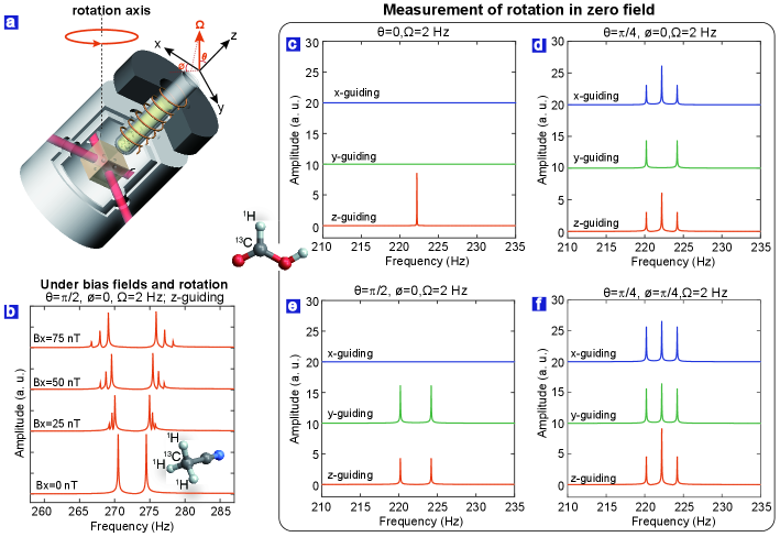
Nuclear spins can also be used to measure inertial rotation. Conventional nuclear spin gyroscopes [40, 41] usually rely on measuring the frequency shift of the freely precessing non-interacting spins (such as ³He) in a bias magnetic field, limiting the gyroscope to detection of rotation along the magnetic field direction. Here, we show that it could overcome this limitation by using strongly interacting nuclear spins, enabling to estimate three dimensional rotations. Similar to magnetic field sensing, strongly interacting nuclear spins can also be sensitive to magnetic pseudo-fields originating from inertial rotation. A magnetic pseudo-field $\mathbf{B}_{\Omega}^{j}=\bm{\Omega}/\gamma_{j}$ is induced on the $j$th spin [40, 59, 60] when the nuclear spin is probed with an atomic vapour sensor in a rotating frame, as shown in Fig. 4a. Here $\bm{\Omega}(\theta,\phi)$ is the rotation vector and parameterized with the polar angle $\theta$ and azimuthal angle $\phi$ and magnitude $\Omega$. The corresponding Hamiltonian is

where $\mathcal{H}_{\textrm{spins}}$ and $\mathcal{H}_{\textrm{int}}$ are described in Eq. (1).

Simulations are performed to investigate the rotational effect on the spectra of ¹³CH_n molecules. Figure 4b shows the spectra of acetonitrile in different magnetic fields and a rotation along the $x$ axis. With decreasing applied magnetic-field strength, the resonance lines gradually change from a multiplet to a doublet. More generally, under inertial rotation and zero magnetic field, arbitrary molecules yield fewer resonance lines than those in real magnetic field [see Eq. (8) in Appendix]. Thus, in contrast to real magnetic field sensing, a variety of molecular species that have no overlapping lines can function as rotation sensors in zero field.

The spectra of strongly interacting nuclear spins can be used to the simultaneous estimation of the rotation speed and the orientation of the rotation axis. As an illustration, we consider the case of nuclear spins initialized with the guiding field along $z$. When the rotation axis is along the sensitive $z$-axis of atomic vapour sensor, the resonance line of formic acid remains a single line (Fig. 4c, bottom). When the rotation axis is along $x$, the resonance line splits into a doublet with a splitting of $2\Omega$ (Fig. 4e, bottom). When the rotation axis is along $\theta=\pi/4$, $\phi=0$, the resonance line splits into a triplet (Fig. 4d, bottom). The above described spectra can still be explained by the theories [see Eqs. (4)-(7) in Appendix] for conventional magnetic field, if $\gamma_{h}\mathbf{B}$ and $\gamma_{c}\mathbf{B}$ are replaced by $\bm{\Omega}$. The measurement of the rotation vector $\bm{\Omega}$ can be performed with the same protocol as the one for the vector magnetometry above. As demonstrations, Figure 4c-f show the simulated spectra of formic acid for four physical rotations with different orientations of the rotation axis. Clearly, they show significant differences. Using the same procedure as for conventional field sensing, we can obtain the rotation frequency and the orientation of the rotation axis. Based on the experimental precision and orientation resolution of our sensor for the real magnetic field, the precision of the rotation frequency is about $2.7\cdot 10^{-4}$ Hz (corresponding to the bias stability of gyroscope [40]) and the rotation orientation resolution is about 0.02 rad. With further optimization (see conclusion and outlook for details), it should be possible to enhance the single-scan precision with several orders of magnitude improvement, which is sufficient for the measurement of Earth’s rotation (about $10^{-5}$ Hz).

In this paper, we have introduced a new approach to multiparameter metrology, using a set of strongly interacting nuclear spins as a quantum resource. Using this technique, we have demonstrated a new type of sensor capable of detecting all three components of a magnetic field or the axis of rotation of an overall sample rotation. This new measurement scheme has promising applications in geophysical surveys, high-precision navigation, and testing fundamental physics. Moreover, our technique naturally avoids the field contamination induced by previously-required reference fields [32, 33, 34, 35], and opens a feasible route towards realizing quantum noise-limited multiparameter sensors.

A further improvement of the experimental sensitivity can be anticipated. For example, the probe states used in this work are thermal equilibrium states with low nuclear-spin polarization. The extension to hyperpolarized states with near-unity spin polarization through many well-developed techniques, such as parahydrogen-induced polarization (PHIP) [61, 62], dynamic nuclear polarization (DNP) [63] and spin-exchange optical pumping (SEOP) [41] techniques, could yield at least five orders of magnitude improvements over currently achievable sensitivity. Moreover, it is also possible to improve the readout sensitivity of the atomic vapour sensor. For example, the application of magnetic gradiometer to the detection of nuclear-spin magnetization, as recently demonstrated in Ref. [52], could enhance the multiparameter estimation sensitivity by a factor of about ten. With recent quantum control technologies [51, 64] in ultralow-field NMR [65, 54, 53, 66], the NOON of the nuclear spins in each molecule can be created which offers an enhanced sensitivity to the multiparameter estimation at a fundamental level [67].

Although demonstrated for strongly-interacting nuclear-spin systems, the protocol presented here can be directly applied to other strongly interacting spin systems and design a new class of multiparameter quantum sensors. We suggest future theoretical and experimental studies of the interaction-based multiparameter metrology with electron-nuclear [68, 69, 70] or electron-electron [71, 72] interacting spin systems, taking a fresh look at many techniques, such as spectroscopy, magnetometry, imaging, navigation, and even biocompass mechanism. For example, the application to nitrogen-vacancy centers [73, 74], which offer the capability of realizing nanometer-scale spatial resolution, could realize a completely new nanometer-scale vector magnetic-field microscope. It can also be applied to explore the magnetic-field orientation dependence of electron-electron spin systems, such as radical pairs in magnetic proteins, which closely relate with the hitherto mysterious biocompass mechanism [71, 72]. We are therefore convinced that this new type of interaction-based multiparameter quantum metrology opens a promising new field of research.

We acknowledge Dmitry Budker, Ren-Bao Liu, Roman P. Frutos and Teng Wu for valuable discussions, and Jiankun Chen for drawing the set-up diagram. This work was supported by National Key Research and Development Program of China (grant no. 2018YFA0306600), National Natural Science Foundation of China (grants nos. 11661161018, 11927811, 12004371), Anhui Initiative in Quantum Information Technologies (grant no. AHY050000), USTC Research Funds of the Double First-Class Initiative (grant no. YD3540002002).

The multiparameter estimation presented in this work includes three stages: probe preparation, encoding with the strongly interacting spins, and probe readout. In the following, we provide the detailed theory of such three stages.

References

- [1] Giovannetti, V., Lloyd, S. & Maccone, L. Advances in quantum metrology. Nat. Photon. 5, 222 (2011).
- [2] Degen, C. L., Reinhard, F. & Cappellaro, P. Quantum sensing. Rev. Mod. Phys. 89, 035002 (2017).
- [3] Pezze, L., Smerzi, A., Oberthaler, M. K., Schmied, R. & Treutlein, P. Quantum metrology with nonclassical states of atomic ensembles. Rev. Mod. Phys. 90, 035005 (2018).
- [4] Braun, D. et al. Quantum-enhanced measurements without entanglement. Rev. Mod. Phys. 90, 035006 (2018).
- [5] Aasi, J. et al. Enhanced sensitivity of the LIGO gravitational wave detector by using squeezed states of light. Nat. Photon. 7, 613–619 (2013).
- [6] Budker, D. & Romalis, M. Optical magnetometry. Nat. Phys. 3, 227–234 (2007).
- [7] Safronova, M. et al. Search for new physics with atoms and molecules. Rev. Mod. Phys. 90, 025008 (2018).
- [8] Lang, J., Liu, R.-B. & Monteiro, T. Dynamical-decoupling-based quantum sensing: Floquet spectroscopy. Phys. Rev. X 5, 041016 (2015).
- [9] Álvarez, G. A., Suter, D. & Kaiser, R. Localization-delocalization transition in the dynamics of dipolar-coupled nuclear spins. Science 349, 846–848 (2015).
- [10] Lucchesi, L. & Chiofalo, M. L. Many-body entanglement in short-range interacting fermi gases for metrology. Phys. Rev. Lett. 123, 060406 (2019).
- [11] Kong, J. et al. Measurement-induced, spatially-extended entanglement in a hot, strongly-interacting atomic system. Nat. Commun. 11, 1–9 (2020).
- [12] Peyronel, T. et al. Quantum nonlinear optics with single photons enabled by strongly interacting atoms. Nature 488, 57–60 (2012).
- [13] Dooley, S., Hanks, M., Nakayama, S., Munro, W. J. & Nemoto, K. Robust quantum sensing with strongly interacting probe systems. NPJ Quant. Inf. 4, 1–7 (2018).
- [14] Nolan, S. P., Szigeti, S. S. & Haine, S. A. Optimal and robust quantum metrology using interaction-based readouts. Phys. Rev. Lett. 119, 193601 (2017).
- [15] Zhou, H. et al. Quantum metrology with strongly interacting spin systems. Phys. Rev. X 10, 031003 (2020).
- [16] Frérot, I. & Roscilde, T. Quantum critical metrology. Phys. Rev. Lett. 121, 020402 (2018).
- [17] Roy, S. & Braunstein, S. L. Exponentially enhanced quantum metrology. Phys. Rev. Lett. 100, 220501 (2008).
- [18] Napolitano, M. et al. Interaction-based quantum metrology showing scaling beyond the Heisenberg limit. Nature 471, 486–489 (2011).
- [19] Boixo, S., Flammia, S. T., Caves, C. M. & Geremia, J. M. Generalized limits for single-parameter quantum estimation. Phys. Rev. Lett. 98, 090401 (2007).
- [20] Zwierz, M., Pérez-Delgado, C. A. & Kok, P. General optimality of the Heisenberg limit for quantum metrology. Phys. Rev. Lett. 105, 180402 (2010).
- [21] Liu, R. et al. Experimental Adiabatic Quantum Metrology with the Heisenberg scaling. arXiv preprint arXiv:2102.07056 (2021).
- [22] Chu, Y., Zhang, S., Yu, B. & Cai, J. Dynamic framework for criticality-enhanced quantum sensing. Phys. Rev. Lett. 126, 010502 (2021).
- [23] Rams, M. M., Sierant, P., Dutta, O., Horodecki, P. & Zakrzewski, J. At the limits of criticality-based quantum metrology: Apparent super-Heisenberg scaling revisited. Phys. Rev. X 8, 021022 (2018).
- [24] Rovny, J., Blum, R. L. & Barrett, S. E. Observation of discrete-time-crystal signatures in an ordered dipolar many-body system. Phys. Rev. Lett. 120, 180603 (2018).
- [25] Kominis, I., Kornack, T., Allred, J. & Romalis, M. V. A subfemtotesla multichannel atomic magnetometer. Nature 422, 596–599 (2003).
- [26] Boixo, S. et al. Quantum metrology: dynamics versus entanglement. Phys. Rev. Lett. 101, 040403 (2008).
- [27] Szczykulska, M., Baumgratz, T. & Datta, A. Multi-parameter quantum metrology. Adv. Phys.: X 1, 621–639 (2016).
- [28] Vidrighin, M. D. et al. Joint estimation of phase and phase diffusion for quantum metrology. Nat. Commun. 5, 1–7 (2014).
- [29] Hou, Z. et al. Zero–trade-off multiparameter quantum estimation via simultaneously saturating multiple Heisenberg uncertainty relations. Sci. Adv. 7, eabd2986 (2021).
- [30] Roccia, E. et al. Multiparameter approach to quantum phase estimation with limited visibility. Optica 5, 1171–1176 (2018).
- [31] Hou, Z. et al. Minimal tradeoff and ultimate precision limit of multiparameter quantum magnetometry under the parallel scheme. Phys. Rev. Lett. 125, 020501 (2020).
- [32] Seltzer, S. & Romalis, M. Unshielded three-axis vector operation of a spin-exchange-relaxation-free atomic magnetometer. Appl. Phys. Lett. 85, 4804–4806 (2004).
- [33] Patton, B., Zhivun, E., Hovde, D. & Budker, D. All-optical vector atomic magnetometer. Phys. Rev. Lett. 113, 013001 (2014).
- [34] Thiele, T., Lin, Y., Brown, M. O. & Regal, C. A. Self-calibrating vector atomic magnetometry through microwave polarization reconstruction. Phys. Rev. Lett. 121, 153202 (2018).
- [35] Li, R. et al. A dual-axis, high-sensitivity atomic magnetometer. Chin. Phys. B 26, 120702 (2017).
- [36] Liu, J. & Yuan, H. Control-enhanced multiparameter quantum estimation. Phys. Rev. A 96, 042114 (2017).
- [37] Spagnolo, N. et al. Quantum interferometry with three-dimensional geometry. Sci. Rep. 2, 1–6 (2012).
- [38] Genovese, M. Real applications of quantum imaging. J. Optics 18, 073002 (2016).
- [39] Komar, P. et al. A quantum network of clocks. Nat. Phys. 10, 582–587 (2014).
- [40] Donley, E. A. Nuclear magnetic resonance gyroscopes. In SENSORS, 2010 IEEE, 17–22 (IEEE, 2010).
- [41] Walker, T. G. & Happer, W. Spin-exchange optical pumping of noble-gas nuclei. Rev. Mod. Phys. 69, 629 (1997).
- [42] Kornack, T., Ghosh, R. & Romalis, M. Nuclear spin gyroscope based on an atomic comagnetometer. Phys. Rev. Lett. 95, 230801 (2005).
- [43] Hurwitz, L. & Nelson, J. Proton vector magnetometer. J. Geophys. Research 65, 1759–1765 (1960).
- [44] Wu, T., Blanchard, J. W., Kimball, D. F. J., Jiang, M. & Budker, D. Nuclear-spin comagnetometer based on a liquid of identical molecules. Phys. Rev. Lett. 121, 023202 (2018).
- [45] Garcon, A. et al. Constraints on bosonic dark matter from ultralow-field nuclear magnetic resonance. Sci. Adv. 5, eaax4539 (2019).
- [46] Jiang, M., Su, H., Garcon, A., Peng, X. & Budker, D. Search for axion-like dark matter with spin-based amplifiers. arXiv preprint arXiv:2102.01448 (2021).
- [47] Hou, Z. et al. “Super-Heisenberg” and Heisenberg Scalings Achieved Simultaneously in the Estimation of a Rotating Field. Phys. Rev. Lett. 126, 070503 (2021).
- [48] Legchenko, A., Baltassat, J.-M., Beauce, A. & Bernard, J. Nuclear magnetic resonance as a geophysical tool for hydrogeologists. J. Appl. Geophys. 50, 21–46 (2002).
- [49] Gross, S. et al. Dynamic nuclear magnetic resonance field sensing with part-per-trillion resolution. Nat. Commun. 7, 1–7 (2016).
- [50] Waters, G. A measurement of the earth’s magnetic field by nuclear induction. Nature 176, 691–691 (1955).
- [51] Jiang, M. et al. Experimental benchmarking of quantum control in zero-field nuclear magnetic resonance. Sci. Adv. 4, eaar6327 (2018).
- [52] Jiang, M. et al. Magnetic gradiometer for the detection of zero-to ultralow-field nuclear magnetic resonance. Phys. Rev. Appl. 11, 024005 (2019).
- [53] Tayler, M. C. et al. Invited review article: Instrumentation for nuclear magnetic resonance in zero and ultralow magnetic field. Rev. Sci. Instrum. 88, 091101 (2017).
- [54] Jiang, M. et al. Interference in atomic magnetometry. Adv. Quantum Technol. 3, 2000078 (2020).
- [55] Béné, G. J. Nuclear magnetism of liquid systems in the earth field range. Phys. Rep. 58, 213–267 (1980).
- [56] Sarkar, R., Ahuja, P., Vasos, P. R. & Bodenhausen, G. Long-lived coherences for homogeneous line narrowing in spectroscopy. Phys. Rev. Lett. 104, 053001 (2010).
- [57] Zeeman, P. The effect of magnetisation on the nature of light emitted by a substance (1897).
- [58] Condon, E. U., Condon, E. & Shortley, G. The theory of atomic spectra (Cambridge University Press, 1935).
- [59] Wood, A. et al. Magnetic pseudo-fields in a rotating electron–nuclear spin system. Nat. Phys. 13, 1070–1073 (2017).
- [60] Heims, S. & Jaynes, E. Theory of gyromagnetic effects and some related magnetic phenomena. Rev. Mod. Phys. 34, 143 (1962).
- [61] Adams, R. W. et al. Reversible interactions with para-hydrogen enhance nmr sensitivity by polarization transfer. Science 323, 1708–1711 (2009).
- [62] Theis, T. et al. Parahydrogen-enhanced zero-field nuclear magnetic resonance. Nat. Phys. 7, 571–575 (2011).
- [63] Maly, T. et al. Dynamic nuclear polarization at high magnetic fields. J. Chem. Phys. 128, 02B611 (2008).
- [64] Jiang, M. et al. Numerical optimal control of spin systems at zero magnetic field. Phys. Rev. A 97, 062118 (2018).
- [65] Ledbetter, M. et al. Near-zero-field nuclear magnetic resonance. Phys. Rev. Lett. 107, 107601 (2011).
- [66] Jiang, M. et al. Zero-to ultralow-field nuclear magnetic resonance and its applications. Fundamental Research 1, 68–84 (2021).
- [67] Jones, J. A. et al. Magnetic field sensing beyond the standard quantum limit using 10-spin noon states. Science 324, 1166–1168 (2009).
- [68] Bermudez, A., Jelezko, F., Plenio, M. B. & Retzker, A. Electron-mediated nuclear-spin interactions between distant nitrogen-vacancy centers. Phys. Rev. Lett. 107, 150503 (2011).
- [69] Zhao, N., Hu, J.-L., Ho, S.-W., Wan, J. T. & Liu, R. Atomic-scale magnetometry of distant nuclear spin clusters via nitrogen-vacancy spin in diamond. Nat. Nanotechnol. 6, 242–246 (2011).
- [70] Schweiger, A. & Jeschke, G. Principles of pulse electron paramagnetic resonance (Oxford University Press on Demand, 2001).
- [71] Xiao, D.-W., Hu, W.-H., Cai, Y. & Zhao, N. Magnetic noise enabled biocompass. Phys. Rev. Lett. 124, 128101 (2020).
- [72] Qin, S. et al. A magnetic protein biocompass. Nat. Mater. 15, 217–226 (2016).
- [73] Shi, F. et al. Sensing and atomic-scale structure analysis of single nuclear-spin clusters in diamond. Nat. Phys. 10, 21–25 (2014).
- [74] Mamin, H. et al. Nanoscale nuclear magnetic resonance with a nitrogen-vacancy spin sensor. Science 339, 557–560 (2013).
- [75] Appelt, S. et al. Paths from weak to strong coupling in nmr. Phys. Rev. A 81, 023420 (2010).
- [76] Sjolander, T. F., Tayler, M. C., King, J. P., Budker, D. & Pines, A. Transition-selective pulses in zero-field nuclear magnetic resonance. J. Phys. Chem. A 120, 4343–4348 (2016).