Multiple pendulum and nonuniform distribution of average kinetic energy

Tetsuro Konishi tkonishi@isc.chubu.ac.jp College of Engineering, Chubu University, Kasugai 487-8501, Japan. Tatsuo Yanagita Department of Engineering Science, Osaka Electro-Communication University, Neyagawa 572-8530, Japan

Abstract

Multiple pendulums are investigated numerically and analytically to clarify the nonuniformity of average kinetic energies of particles. The nonuniformity is attributed to the system having constraints and it is consistent with the generalized principle of the equipartition of energy. With the use of explicit expression for Hamiltonian of a multiple pendulum, approximate expressions for temporal and statistical average of kinetic energies are obtained, where the average energies are expressed in terms of masses of particles. In a typical case, the average kinetic energy is large for particles near the end of the pendulum and small for those near the root. Moreover, the exact analytic expressions for the average kinetic energy of the particles are obtained for a double pendulum.

I Introduction

Pendulums are useful to explore the fundamental behavior of various physical systems. A simple pendulum is a good example of a system that can demonstrate periodic motion Galilei (1638). When the amplitude of the oscillation is small, i.e., the total energy is small, the periodic motion of a simple pendulum is well approximated by that of a harmonic oscillator, wherein the period of the oscillation does not depend on the amplitude Goldstein (1980).

The fundamental modes and principle of superposition can be understood by studying a double pendulum Bernoulli (1738, 1740); Cannon and Dostrovsky (1981); Goldstein (1980). When the amplitude of oscillation is small, there are two special motions called the fundamental modes, wherein both the upper and lower pendulums oscillate in the same period. For a small-amplitude oscillation, one can understand that every motion of the double pendulum is expressed by the superposition of the two fundamental modes. The principle of superposition is a key concept for understanding various linear phenomena. Since both fundamental modes of the double pendulum indicates periodic motion, the double pendulum exhibits periodic or quasiperiodic motion when the amplitudes are small.

Meanwhile, a double pendulum is also a good example of a system that indicates chaotic motion Lichtenberg and Lieberman (1992); Ott (2002); Tabor (1989); Shinbrot et al. (1992); Stachowiak and Okada (2006); Shinbrot et al. (1992); Rafat et al. (2009); Dullin (1994); Stachowiak and Szumiński (2015); Ivanov (1999, 2001a, 2000, 2001b). If a large energy is assigned and the amplitudes of displacements are not small, the motion of a double pendulum is no longer regular, and chaotic behavior is observed. Multiple pendulums with three or more degrees of freedom Bernoulli (1738, 1740); Cannon and Dostrovsky (1981) also exhibit chaotic behavior Oyama and Yanagita (1998); Saitoh et al. (1999); Saitoh and Yanagita (2000).

When chaos is strong in a multiple pendulum, one can expect that it admits a statistical description; the long time average of the physical quantity is considered to be approximately equal to the average over the energy surface. Then, each particle in the pendulum can be considered as a subsystem connected to a heat bath that comprises the rest of the pendulum; then, the particles are in a thermal equilibrium.

One may expect that the sytem in thermal equilibrium is almost uniform. However, a careful observation of the motions of a multiple pendulum indicate that the particle at the end of the pendulum moves faster than the particle nearest to the root of the pendulum, even if the masses of all particles are the same. In fact, one author conducted numerical computations and revealed that the time average of the kinetic energies of a multiple pendulum are different Oyama and Yanagita (1998); Saitoh et al. (1999); Saitoh and Yanagita (2000). In this paper, we revisit the observation and explain the origin of differences in the average kinetic energies using the generalized principle of the equipartition of energy Tolman (1918, 1938); Kubo et al. (1990); Konishi and Yanagita (2009). The nonuniformity of the average kinetic energy is consistent with the generalized principle of equipartition of energy. Thus, the average kinetic energy can be nonuniform under a thermal equilibrium.

The remainder of this paper is organized as follows. In Section II, we describe our model, a multiple pendulum. Then, we provide an explicit form of the Lagrangian and Hamiltonian of a multiple pendulum. In Section III, we present the results of numerical computation where the values of time-average kinetic energies of particles in the multiple pendulum are not equal, at the same time the generalized principle of equipartition holds. In Section IV, we explain the nonuniform distribution of average kinetic energy based on statistical mechanics; further, an exact expression is obtained for the double pendulum. Finally, Section V presents the summary and the discussions.

II Model

The multiple pendulum examined in this study is composed of $N$ particles serially connected by $N$ massless links of fixed length in a uniform gravitational field, as illustrated in Fig.1. One end is fixed to a point we define as the origin $(0,0)$ . The particles and links pass through each other if they arrive at the same position. The particles move in a fixed vertical plane, which is defined as the $xy$ -plane. The $x$ -axis is considered to be in the horizontal direction, and the $y$ -axis, in the vertical direction with the upward direction representing the positive $y$ direction. We let $m_{i}$ , $\overrightarrow{r_{i}}\equiv(x_{i},y_{i})$ , and $\ell_{i}$ represent the mass of the $i$ ’th particle, position of the $i$ ’th particle, and length of $i$ ’th link, respectively. $g$ represents the constant of gravitational acceleration. The distance between $i$ ’th and $i+1$ ’th particles is fixed for all $i$ . In this sense, the system has constraints.

In terms of the Cartesian coordinates $(x_{i},y_{i})$ , the kinetic energy of the $i$ ’th particle $K_{i}$ , total kinetic energy $K$ , and potential energy $U$ are

$\displaystyle K_{i}$	$\displaystyle=\frac{m_{i}}{2}(\dot{x}_{i}^{2}+\dot{y}_{i}^{2})\ ,$	(1)
$\displaystyle K$	$\displaystyle=\sum_{i=1}^{N}K_{i}\ ,$	(2)
$\displaystyle U$	$\displaystyle=\sum_{i=1}^{N}m_{i}gy_{i}\ .$	(3)

Using these equations, the system is defined by a Lagrangian $L$ and constraints $G_{i}$ , which are given as

	$\displaystyle L$	$\displaystyle=K-U=\sum_{i=1}^{N}\frac{m_{i}}{2}\left(\dot{x}_{i}^{2}+\dot{y}_{i}^{2}\right)-\sum_{i=1}^{N}m_{i}gy_{i}\ ,$		(4)
	$\displaystyle G_{i}$	$\displaystyle\equiv\left\|\overrightarrow{r_{i}}-\overrightarrow{r_{i-1}}\right\|^{2}-\ell_{i}^{2}=0\ ,i=1,2,\cdots,N,$		(5)

where $\overrightarrow{r_{0}}\equiv(x_{0},y_{0})\equiv(0,0)$ and a dot over each symbol represents derivative with respect to time e.g., $\dot{x}_{i}=\frac{dx}{dt}$ .

Refer to caption — Figure 1: Multiple pendulum: Definition of variables and parameters

If we denote $\varphi_{i}$ as the angle between the $i$ ’th link and the $-y$ direction (direction of gravity), we have

	$\displaystyle x_{i}$	$\displaystyle=x_{i-1}+\ell_{i}\sin\varphi_{i}\ \ =\sum_{j=1}^{i}\ell_{j}\sin\varphi_{j},$		(6)
	$\displaystyle y_{i}$	$\displaystyle=y_{i-1}-\ell_{i}\cos\varphi_{i}\ \ =-\sum_{j=1}^{i}\ell_{j}\cos\varphi_{j}\,.$		(7)

The Lagrangian (4) is then expressed in terms of $\varphi_{i}$ , $i=1,2,\cdots,N$ as

$\displaystyle L$	$\displaystyle=K-U\ ,$	(8)
$\displaystyle K$	$\displaystyle=\sum_{i,j=1}^{N}\frac{1}{2}A(\varphi)_{ij}\dot{\varphi}_{i}\dot{\varphi}_{j}\ ,$	(9)
$\displaystyle U$	$\displaystyle=-\sum_{i=1}^{N}m_{i}g\sum_{j=1}^{i}\ell_{j}\cos\varphi_{j}\ ,$	(10)

where the $N\times N$ matrix $A$ is defined as

A(\varphi)_{nk}\equiv\left(\sum_{i=\max(n,k)}^{N}m_{i}\right)\ell_{n}\ell_{k}\cos(\varphi_{n}-\varphi_{k})\ \ .

(11)

The derivations of Eqs. (9) and (11) are presented in Appendix A.

Using Eqs.(6) and (7), $K_{i}$ can be expressed in the quadratic form of $\dot{\varphi}$ as

	$\displaystyle K_{i}$	$\displaystyle=\frac{m_{i}}{2}\sum_{j=1}^{i}\sum_{k=1}^{i}\dot{\varphi}_{j}\dot{\varphi}_{k}\ell_{j}\ell_{k}\cos(\varphi_{j}-\varphi_{k})$		(12)
		$\displaystyle=\frac{1}{2}\sum_{j,k}A_{jk}^{(i)}\dot{\varphi}_{j}\dot{\varphi}_{k}$		(13)

where $A^{(i)}$ represents a $N\times N$ matrix defined as

A_{jk}^{(i)}=\begin{cases}m_{i}\ell_{j}\ell_{k}\cos(\varphi_{j}-\varphi_{k})&\cdots j\leq i\ \text{and}\ k\leq i\ ,\\ 0&\cdots\text{otherwise}\ .\end{cases}

(14)

Because $\sum_{i}K_{i}=K$ , the sum of $A^{(i)}$ with respect to $i$ is equal to the matrix $A$ :

\sum_{i=1}^{N}A_{jk}^{(i)}=A_{jk}\ .

(15)

Matrices $A$ and $A^{(i)}$ depend on coordinates $\varphi$ .

The momentum $p_{i}$ canonically conjugate to the coordinate $\varphi_{i}$ is defined as

p_{i}\equiv\displaystyle\frac{\partial L}{\partial\dot{\varphi}_{i}}\ .

(16)

Then, we have

	$\displaystyle p_{n}$	$\displaystyle=\sum_{k=1}^{N}A_{nk}\dot{\varphi}_{k}\,,$		(17)
	$\displaystyle K$	$\displaystyle=\frac{1}{2}\sum_{j,k}p_{j}A^{-1}_{jk}p_{k}\ .$		(18)

$K_{i}$ using momentum $p$ is expressed as

K_{i}=\frac{1}{2}\sum_{j,k,\xi,\eta}A_{jk}^{(i)}A^{-1}_{j\xi}A^{-1}_{k\eta}p_{\xi}p_{\eta}\ ,

(19)

Using Eq.(18), the Hamiltonian of a multiple pendulum is given as

H=\frac{1}{2}\sum_{j,k=1}^{N}p_{j}A^{-1}_{jk}p_{k}-\sum_{i=1}^{N}m_{i}g\sum_{j=1}^{i}\ell_{j}\cos\varphi_{j}\ .

(20)

III Numerical Example

III.1 Simulation Method

First, let us explain the methods of numerical simulation using which we integrate the equation of motion of the multiple pendulum. The equation of motion derived from the Lagrangian written in terms of $\varphi$ is complicated because of the dependence of the kinetic energy on $\varphi$ . Hence, we use the equation of motion written in terms of the Cartesian coordinates $xy$ derived from Eqs.(4) and (5). The equation of motion includes the terms from the constraint characterized by the coefficients called “Lagrange multipliers” Goldstein (1980). We numerically evaluate the Lagrange multipliers at each step of the integration to ensure that the constraints in Eq.(5) are satisfied. The idea used in this method is the same as that in the “RATTLE” algorithm Leimkuhler and Reich (2004); http://www.charmm.org/ ; Vesely (2013). We use the fourth-order symplectic integrator composed of three second-order symplectic integrators Leimkuhler and Reich (2004); Yoshida (1990) incorporating forces from the constraints.

We calculate the kinetic energies of the particles of the multiple pendulum. Let us denote $K_{i}(t)$ as the kinetic energy of the $i$ ’th particle (Eq.(1)) at time $t$ . The time average of $K_{i}(t)$ is defined as

\overline{K_{i}}(t)\equiv\frac{1}{t}\int_{0}^{t}K_{i}(t^{\prime})\,dt^{\prime}\ .

(21)

III.2 Simulation Results

Let us observe some typical time evolutions of the multiple pendulum obtained from the numerical simulation. Here, we adopt the initial condition $\dot{x}_{i}(0)=\dot{y}_{i}(0)=0$ for all $i$ ; $\varphi_{i}(0)=\theta$ for all $i$ . This is a stretched configuration with angle $\theta$ .

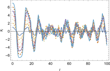
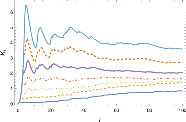
Let us consider the initial angle as $\theta=\pi/2$ . The top panel of Fig.2 shows the chaotic motion after a short transient; the bottom panel shows the temporal evolution of the average kinetic energies $\overline{K_{i}}(t)$ . Further, $\overline{K_{i}}(t)$ does not converge to a single value; on the contrary, they converge to different values, i.e., the average kinetic energy is not uniform.

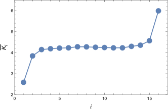
The nonuniformity in the $\overline{K_{i}}$ remains even if we take a longer time for averaging. Fig. 3 shows a plot of the average kinetic energy of each particle $\overline{K_{i}}$ (Eq.(21)) against $i$ for $N=16$ . The values of $\overline{K_{i}}$ are not the same. The $\overline{K_{i}}$ of particles near the end are large, whereas those of particles near the root are small. This is consistent with Yanagita et al.’s first observation Oyama and Yanagita (1998); Saitoh et al. (1999); Saitoh and Yanagita (2000).

III.3 Non-uniformity of Average Kinetic Energy and the Generalized Principle of the Equipartition of Energy

Let us consider the relation between the non-uniformity of $\overline{K_{i}}$ we observed in the previous subsection and the generalized principle of the equipartition of energy Tolman (1918, 1938); Kubo et al. (1990); Konishi and Yanagita (2009).

It is natural to assume that the set of points $\left(\varphi_{i}(t),p_{i}(t)\right),i=1,2,\cdots,N$ generated from the time series is close to the microcanonical ensemble because the motion of the multiple pendulum considered in this study is highly chaotic. Further, each single particle in the multiple pendulum can be regarded as a subsystem attached to a “heat bath” composed of the rest of the pendulum ( $N-1$ particles), and we can roughly approximate the statistical distribution of the state of the single particle as a canonical distribution at some temperature. This assumption allows us to interpret the original phenomena of the nonuniformity of the temporal average $\overline{K_{i}}$ as the nonuniformity of the thermal average $\left\langle K_{i}\right\rangle$ . Below, we explain the nonuniformity of the thermal average using the generalized principle of the equipartition of energy.

Eq.(9) shows that the kinetic energy of the system has off-diagonal elements that depend on the coordinate $\varphi$ . Thus, we cannot apply the ordinary form of the principle of the equipartition of energy. Instead, we use the generalized principle of the equipartition of energy, which states

\left<K_{i}^{(c)}\right>=\frac{1}{2}k_{B}T\ .

(22)

Here, $T$ represents the temperature, $k_{B}$ denotes Boltzmann’s constant, the bracket $\left\langle\cdots\right\rangle$ represents the thermal average, and $K_{i}^{(c)}$ is defined as

K_{i}^{(c)}\equiv\frac{1}{2}p_{i}\displaystyle\frac{\partial K}{\partial p_{i}},

(23)

where $p_{i}$ represents the momentum canonically conjugate to the coordinate $\varphi_{i}$ . In Eq.(23), the summation with respect to $i$ is not considered. We call $K_{i}$ and $K_{i}^{(c)}$ the “linear kinetic energy” and “canonical kinetic energy”, respectively.

For the multiple pendulum, $K_{i}^{(c)}$ (Eq.(23)) is

K_{i}^{(c)}=\sum_{k=1}^{N}\frac{1}{2}p_{i}A^{-1}_{ik}p_{k}\,.

(24)

This is different from the kinetic energy of the $i$ ’th particle $K_{i}$ defined in (Eq.(19)), hence

K_{i}\neq K_{i}^{(c)}\ .

(25)

Using Eqs. (22) and (25), $\left\langle K_{i}\right\rangle$ , the average of $K_{i}$ , does not take the same value at the thermal equilibrium in general.

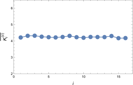
Fig. 4 shows the time average of canonical kinetic energy Eq.(23) of the multiple pendulum using the same time series as in Fig. 3. Here, we can see that $\overline{K_{i}^{(c)}}$ takes almost the same value and the generalized principle of the equipartition of energy is realized. That is, even when the thermal equilibrium is established and the generalized principle of equipartition of energy holds, the average of $K_{i}$ takes different values and the nonuniformity of the average kinetic energy is realized in the thermal equilibrium.

IV Analytical explanation

IV.1 Temporal average

If we denote

\Delta x_{i}\equiv x_{i}-x_{i-1}\ ,\ \Delta y_{i}\equiv y_{i}-y_{i-1}\ ,

(26)

Eq.(24), the “canonical kinetic energy” of the $i$ ’th degree of freedom, is expressed as

K_{i}^{c}=\sum_{j=1}^{N}\frac{1}{2}\left(\sum_{n=\max(i,j)}^{N}m_{n}\right)\left[\Delta\dot{x}_{i}\Delta\dot{x}_{j}+\Delta\dot{y}_{i}\Delta\dot{y}_{j}\right]\ \ .

(27)

where $\Delta\dot{x}_{1}=\dot{x}_{1}$ and $\Delta\dot{y}_{1}=\dot{y}_{1}$ because $x_{0}\equiv y_{0}\equiv 0$ . Detail of calculation is shown in Appendix B.

Let us assume

\overline{\Delta\dot{x}_{i}\Delta\dot{x}_{j}}=0\ ,\ \overline{\Delta\dot{y}_{i}\Delta\dot{y}_{j}}=0\ \ (i\neq j)\ .

(28)

This assumption implies that each link in the multiple pendulum rotates statistically independently.

Then, we have by straightforward calculation that

	$\displaystyle\overline{K_{i}^{c}}$	$\displaystyle=\frac{1}{2}\left(\sum_{n=i}^{N}m_{n}\right)\left[\left(\overline{\dot{x}_{i}^{2}}+\overline{\dot{y}_{i}^{2}}\right)-\left(\overline{\dot{x}_{i-1}^{2}}+\overline{\dot{y}_{i-1}^{2}}\right)\right]$		(29)
		$\displaystyle=\left(\sum_{n=i}^{N}m_{n}\right)\left(\frac{1}{m_{i}}\overline{K_{i}}-\frac{1}{m_{i-1}}\overline{K_{i-1}}\right)\ .$		(30)

Assuming that the temporal average $\overline{K^{c}_{i}}$ is equal to the thermal average $\left<K^{c}_{i}\right>$ and using the generalized principle of equipartition of energy Tolman (1918, 1938); Kubo et al. (1990) for the “canonical kinetic energy” we have $\overline{K^{c}_{i}}=\frac{1}{2}k_{B}T$ , and the long time average of “linear kinetic energy” of the $i$ ’th particle $K_{i}$ is recursively expressed as

\overline{K_{i}}=\frac{m_{i}}{m_{i-1}}\,\overline{K_{i-1}}+\frac{m_{i}}{\sum_{n=i}^{N}m_{n}}\,\cdot\frac{1}{2}k_{B}T\ .

(31)

Since $(x_{0},y_{0})=(0,0)$ and $K_{0}\equiv 0$ , we have

\overline{K_{i}}=m_{i}\left(\sum_{j=1}^{i}\frac{1}{\sum_{n=i}^{N}m_{n}}\right)\cdot\frac{1}{2}k_{B}T\,.

(32)

Hence, the temporal average of the kinetic energy is nonuniform.

If all masses have the same value $m_{1}=m_{2}=\cdots=m_{N}$ , then $\overline{K_{n}}$ ’s are explicitly expressed as

\overline{K_{i}}=\left(\sum_{j=1}^{i}\frac{1}{N-j+1}\right)\frac{k_{B}T}{2}

(33)

so that the average linear kinetic energies $\overline{K_{i}}$ can monotonically increase from the root to the end of the pendulum as

\overline{K_{1}}<\overline{K_{2}}<\cdots<\overline{K_{N}}\ .

(34)

This is consistent with the numerical results shown in Fig. 3.

IV.2 Statistical Average

The nonuniformity of the average energy can be explained using a statistical method. Suppose the system is under thermal equilibrium at temperature $T$ . The statistical average of the linear kinetic energy $K_{i}$ is then defined as

\left<K_{i}\right>\equiv\frac{1}{Z}\int K_{i}e^{-\beta H}d\Gamma\,,

(35)

where $Z\equiv\int e^{-\beta H}d\Gamma$ , $\beta\equiv 1/k_{B}T$ , and $d\Gamma\equiv d^{N}\!p\,d^{N}\!\varphi$ .

Using the expression for $K_{i}$ ,

\left<K_{i}\right>=\frac{m_{i}}{2}\sum_{j=1}^{i}\sum_{k=1}^{i}\ell_{j}\ell_{k}\left<\dot{\varphi}_{j}\dot{\varphi}_{k}\cos\varphi_{jk}\right>\ ,

(36)

where $\varphi_{jk}\equiv\varphi_{j}-\varphi_{k}$ .

Using Eq.(19), we can express Eq.(36) in terms of the canonical momenta $p_{i}$ as

\left\langle K_{i}\right\rangle=\frac{1}{2}\sum_{j,k,\xi,\eta}\left\langle A_{jk}^{(i)}A^{-1}_{j\xi}A^{-1}_{k\eta}p_{\xi}p_{\eta}\right\rangle\ .

(37)

Integrating by parts with respect to $p$ yields

	$\displaystyle\left\langle K_{i}\right\rangle$	$\displaystyle=\frac{1}{2\beta}\left\langle\mbox{tr}\left(A^{(i)}A^{-1}\right)\right\rangle$		(38)
		$\displaystyle=\frac{1}{2\beta}\frac{1}{Z}\int\mbox{tr}\left(A^{(i)}A^{-1}\right)e^{-\beta\left(\frac{1}{2}pA^{-1}p+U(\varphi)\right)}d\Gamma\ .$		(39)

Here, matrices $A^{-1}$ and $A^{(i)}$ depend on $\varphi$ .

In Eq.(39), we first perform integration with respect to $p$ , which is a multidimensional Gaussian integral. The result is

\int e^{-\beta\left(\frac{1}{2}pA^{-1}p\right)}d^{N}p=\left(\frac{2\pi}{\beta}\right)^{N/2}\sqrt{\det A}\ .

(40)

Hence, we have

	$\displaystyle Z$	$\displaystyle=\left(\frac{2\pi}{\beta}\right)^{N/2}\int\sqrt{\det A}\,e^{-\beta U(\varphi)}d^{N}\varphi\ ,$		(41)
	$\displaystyle\left\langle K_{i}\right\rangle$	$\displaystyle=\frac{1}{2\beta}\frac{\int\mbox{tr}\left(A^{(i)}A^{-1}\right)\sqrt{\det A}\,e^{-\beta U(\varphi)}d^{N}\varphi}{\int\sqrt{\det A}\,e^{-\beta U(\varphi)}d^{N}\varphi}\ .$		(42)

In the following, we use these equations to express $\left\langle K_{i}\right\rangle$ for multiple and double pendulums.

IV.2.1 Multiple Pendulum with an arbitrary number of particles

Let us adopt “diagonal approximation”

\left<\dot{\varphi}_{j}\dot{\varphi}_{k}\cos\varphi_{jk}\right>=0\ \text{for}\ j\neq k\,,

(43)

and

\left<A^{-1}_{jj}\right>\approx\left<\frac{1}{A_{jj}}\right>=\frac{1}{\left(\sum_{i=j}^{N}m_{i}\right)\ell_{j}^{2}}\ .

(44)

These approximations assumes that each link rotates statistically independently, and we omit all non-diagonal elements of matrix $A$ , where phase factors such as $\cos(\varphi_{i}-\varphi_{j})$ are included.

Then, we obtain

\left<K_{i}\right>=m_{i}\left(\sum_{j=1}^{i}\frac{1}{\sum_{n=j}^{N}m_{n}}\right)\cdot\frac{1}{2}k_{B}T\,.

(45)

This expression is equivalent to that in Eq.(32) if the thermal average on the left-hand side $\left<\cdots\right>$ is replaced by the time average $\overline{\cdots}$ . The details of the calculation are summarized in Appendix C.

This result indicates that when all masses are the same, the average linear kinetic energies are monotonically increasing from the root to the end of the pendulum, as shown in Fig. 3.

\left<K_{1}\right><\left<{K_{2}}\right><\cdots<\left<{K_{N}}\right>\ .

(46)

IV.2.2 Double pendulum

For the case of the double pendulum, i.e., for the $N=2$ case, we can obtain the exact expressions for $\left\langle K_{i}\right\rangle$ .

For $N=2$ , matrices $A$ , $A^{(i)}$ , defined by Eqs. (11) and (15), respectively, and $\det A$ reads

$\displaystyle A$	$\displaystyle=M\begin{pmatrix}\ell_{1}^{2}&\mu_{2}\ell_{1}\ell_{2}C_{12}\\ \mu_{2}\ell_{1}\ell_{2}C_{12}&\mu_{2}\ell_{2}^{2}\end{pmatrix}\ ,$	(47)
$\displaystyle A^{(1)}$	$\displaystyle=M\mu_{1}\ell_{1}^{2}\begin{pmatrix}1&0\\ 0&0\end{pmatrix}\ ,$	(48)
$\displaystyle A^{(2)}$	$\displaystyle=M\mu_{2}\begin{pmatrix}\ell_{1}^{2}&\ell_{1}\ell_{2}C_{12}\\ \ell_{1}\ell_{2}C_{12}&\ell_{2}^{2}\end{pmatrix}\ ,$	(49)
$\displaystyle\det A$	$\displaystyle=M^{2}\mu_{2}\ell_{1}^{2}\ell_{2}^{2}\left(1-\mu_{2}C_{12}^{2}\right)\ ,$	(50)

where

$\displaystyle C_{12}$	$\displaystyle=\cos(\varphi_{2}-\varphi_{1})\ ,$	(51)
$\displaystyle M$	$\displaystyle=m_{1}+m_{2}\ ,$	(52)
$\displaystyle\mu_{i}$	$\displaystyle=m_{i}/M\ .$	(53)

From these, we obtain

	$\displaystyle\mbox{tr}\left(A^{(1)}A^{-1}\right)$	$\displaystyle=\frac{\mu_{1}}{1-\mu_{2}C_{12}^{2}}\ ,$		(54)
	$\displaystyle\mbox{tr}\left(A^{(2)}A^{-1}\right)$	$\displaystyle=\frac{(1+\mu_{2})-2\mu_{2}C_{12}^{2}}{1-\mu_{2}C_{12}^{2}}=2-\mbox{tr}\left(A^{(1)}A^{-1}\right)\ .$		(55)

Here, we used $\mu_{1}+\mu_{2}=1$ .

We obtain the exact expressions of $\left\langle K_{i}\right\rangle$ for a double pendulum by substituting these into Eq.(42) and expanding $\det A$ as a series of $\mu_{2}C_{12}^{2}$ .

	$\displaystyle\left\langle K_{1}\right\rangle$	$\displaystyle=\frac{1}{2\beta}\frac{\displaystyle\mu_{1}\sum_{n=0}^{\infty}\frac{(2n-1)!!}{n!2^{n}}\mu_{2}^{n}R_{n}(\alpha_{1},\alpha_{2})}{\displaystyle I_{0}(\alpha_{1})I_{0}(\alpha_{2})-\sum_{n=1}^{\infty}\frac{(2n-3)!!}{n!2^{n}}\mu_{2}^{n}R_{n}(\alpha_{1},\alpha_{2})}\ ,$		(56)
	$\displaystyle\left\langle K_{2}\right\rangle$	$\displaystyle=\frac{1}{\beta}-\left\langle K_{1}\right\rangle\ ,$		(57)

where

$\displaystyle R_{n}(\alpha_{1},\alpha_{2})$	$\displaystyle=\sum_{j=0}^{n}{}_{2n}C_{2j}\left\{(2(n-j)-1)!!\right\}^{2}$
	$\displaystyle\cdot\left\{\frac{\partial^{2j}}{\partial\alpha_{1}^{2j}}\left(\frac{I_{n-j}(\alpha_{1})}{\alpha_{1}^{n-j}}\right)\right\}\left\{\frac{\partial^{2j}}{\partial\alpha_{2}^{2j}}\left(\frac{I_{n-j}(\alpha_{2})}{\alpha_{2}^{n-j}}\right)\right\}$	(58)
$\displaystyle\alpha_{1}$	$\displaystyle=\beta(m_{1}+m_{2})g\ell_{1},$	(59)
$\displaystyle\alpha_{2}$	$\displaystyle=\beta m_{2}g\ell_{2},$	(60)

and $I_{n}(z)$ is the modified Bessel function of the $n$ ’th order DLM .

Fig. 5 shows the values of $\left\langle K_{i}\right\rangle$ , $i=1,2$ , calculated from Eqs.(56) and (57). We show the result of Eq.(35) obtained from Markov Chain Monte Carlo method by symbols to check the validity of Eqs.(56) and (57). We see that both calculations agree quite well.

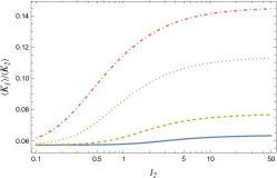
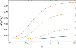
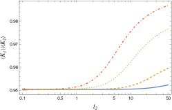
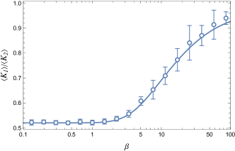
Fig. 5 shows that $\beta\cdot\left\langle K_{i}\right\rangle$ appear to converge to certain finite values as $\beta\rightarrow 0$ . In fact, they are calculated as

\displaystyle\lim_{\beta\rightarrow 0}\beta\cdot\left\langle K_{1}\right\rangle

\displaystyle=\frac{\mu_{1}}{2}\frac{K(\sqrt{\mu_{2}})}{E(\sqrt{\mu_{2}})}\ ,

(61)

and $\lim_{\beta\rightarrow 0}\beta\cdot\left\langle K_{2}\right\rangle$ is calculated from Eq.(57). Here, $K(k)$ and $E(k)$ represent the complete elliptic integrals of the 1st and 2nd kind DLM , respectively. The calculation of Eq.(61) is presented in Appendix D. From this, we see that, the average kinetic energies do not depend on $\ell_{i}$ or $g$ at the high-temperature limit. This is similar to the approximate expression in Eq.(45).

When $m_{1}=m_{2}$ , i.e., $\mu_{1}=\mu_{2}=1/2$ , we see that

	$\displaystyle\lim_{\beta\rightarrow 0}\beta\cdot\left\langle K_{1}\right\rangle$	$\displaystyle=0.3431\cdots\ ,$		(62)
	$\displaystyle\lim_{\beta\rightarrow 0}\beta\cdot\left\langle K_{2}\right\rangle$	$\displaystyle=0.6568\cdots\ .$		(63)

These values agree well with the values obtained from the Markov Chain Monte Carlo method, as shown in Fig. 5.

Now that we have obtained the exact expression for $\left\langle K_{i}\right\rangle$ , we can analyze their dependence on the parameters.

In Fig. 6, we show the $\ell_{2}$ dependence of the ratio $\left\langle K_{1}\right\rangle/\left\langle K_{2}\right\rangle$ for $\mu_{1}=0.05$ , $0.5$ , and $0.95$ . In every case, as $\ell_{2}$ increases, that is, the length of the lower pendulum increases, the ratio $\left\langle K_{1}\right\rangle/\left\langle K_{2}\right\rangle$ increases.

In Figure 7, we plot the $\beta$ dependence of the ratio $\left\langle K_{1}\right\rangle/\left\langle K_{2}\right\rangle$ . We see that for $\beta\rightarrow 0$ , the ratio converges to a positive value, and around $\beta\sim 1$ , the ratio increases gradually.

In these figures, we note two remarkable features:

(i) At every temperature we have $\left\langle K_{1}\right\rangle<\left\langle K_{2}\right\rangle$ . That is, the particle at the end of the pendulum has a larger average kinetic energy than the other particle near the root.
(ii) The difference between the average kinetic energies is large for high temperatures and small for low temperatures, and a crossover temperature is observed near $\beta=1$ .

The first feature is proved as follows. From Eq.(54) and $\mu_{1}+\mu_{2}=1$ , we have

0\leq\mbox{tr}\left(A^{(1)}A^{-1}\right)\leq 1\leq\mbox{tr}\left(A^{(2)}A^{-1}\right)\leq 2\ .

(64)

Eqs.(64) and (38) indicate that

0\leq\left\langle K_{1}\right\rangle\leq\frac{1}{2\beta}\leq\left\langle K_{2}\right\rangle\leq\frac{1}{\beta}\

(65)

for any values of parameters $m_{i}$ , $\ell_{i}$ , and for any temperature. Hence, the particle at the end always has a larger average kinetic energy than the other particle for a double pendulum.

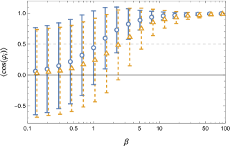
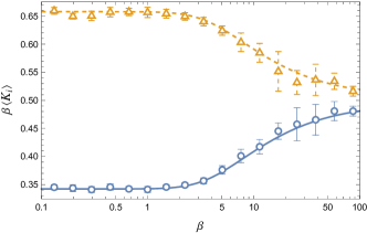
Let us consider the latter feature. In Fig.8, we show $\left\langle\cos\varphi_{i}\right\rangle$ calculated by the Markov Chain Monte Carlo method. We observe that for high temperatures $\beta\sim 0$ , $\left\langle\cos\varphi_{i}\right\rangle\sim 0$ for both $i=1$ and $i=2$ . Hence, angles take various values, and the pendulum shows the rotational motion. For low temperature $\beta\gg 1$ , $\left\langle\cos\varphi_{i}\right\rangle\sim 1$ that is, $\varphi_{i}\sim 0$ for both $i=1$ and $i=2$ ; the pendulum exhibits a small-angle liberation. Hence, the crossover temperature observed in Fig.5 is related to crossover between the librational and rotational motions of the pendulum.

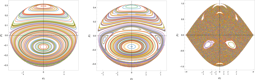
The change in the motion was observed by examining the Poincaré surface of the section of the double pendulum. Fig. 9 shows the Poincaré surface of section $(\varphi_{2},p_{2})$ taken at $\varphi_{1}=0$ and $p_{1}-p_{2}\cos\varphi_{2}>0$ for several values of the total energy. Definition of the section is explained in Appendix E. As the total energy $E$ approaches $E\sim 1$ , the chaotic region in the phase space rapidly expands and fills most of the energy surface. Hence, we interpret the crossover near $\beta~{}\sim 1$ found in previous figures as the change in motion from the limited librational to the strongly chaotic motion.

V Summary and discussions

We showed that the averages of the linear kinetic energies of particles in multiple pendulum take different values via numerical computation and analytical calculations. Since the multiple pendulum has constraints, uniformity of average kinetic energy of each particle at thermal equilibrium is no longer guaranteed. On the contrary, another quantity what we call canonical kinetic energy is uniform, and the uniformity is guaranteed by the generalized principle of equipartition of energy. Moreover, the uniformity of the average canonical kinetic energy yields non-uniformity of the average kinetic energy of each particle.

Systems with constraints do not obey the (conventional) principle of the equipartition of energy, but a generalized one. Our discovery added a new example in which we can see how the system systematically deviates from (not generalized) equipartition Konishi and Yanagita (2009).

The average linear kinetic energy of each particle was not the same because of the difference between the linear and canonical kinetic energies. The difference comes from the fact that the kinetic energy depends on coordinates; this dependence is attributed to the existence of constraints. In short, the constraints give rise to the nonuniform distribution of the average linear kinetic energies. This scenario is similar to a chain system without a fixed root, i.e., a freely jointed chain. Freely jointed chain is a simplified model of polymers and is composed of particles connected by massless rigid links Kuhn (1934); Kuhn and Kuhn (1948); Kramers (1946); Fixman (1974); Fixman and Kovac (1974); Mazars (1996); Doi and Edwards (1988); Doi (1996); Strobl (1997); Siegert et al. (1993). For a freely jointed chain, the average kinetic energy of each particle is large near both ends of the chain and small near the middle of the chain Konishi and Yanagita (2009).

For a double pendulum, we successfully obtained the exact expressions for $\left\langle K_{i}\right\rangle$ . They include temperature, mass of two particles, lengths of two links, and gravitational constant. Hence, the exact expression is useful to design a system that has predefined values of average kinetic energy. Exact expressions for average kinetic energies are also obtained for a three-particle two-dimensional freely jointed chain Konishi and Yanagita , where non-uniformity of the average kinetic energies is also shown.

Further, we showed that the dependence of $\beta\cdot\left\langle K_{i}\right\rangle$ on the mass and length of links vanishes in the high-temperature limit. The reason why $\beta\cdot\left\langle K_{i}\right\rangle$ does not depend on $\ell_{i}$ or $g$ is interpreted as follows: $\left\langle K_{i}\right\rangle$ depends on $\ell_{i}$ or $g$ only through coupling with $\beta$ , as in Eq.(59) and (60). Hence, in the limit $\beta\rightarrow 0$ , the dependence on $\ell_{i}$ or $g$ vanishes. This independence is also observed in the approximate expression in Eq.(45). Thus, the approximation adopted to obtain Eq.(45) is similar to the high-temperature approximation.

In this paper we considered a multiple pendulum which have constraints, and the constraints are essential for non-uniformity of average kinetic energies. In real systems there are no exact constraints; constraints appearing in models are often approximations of stiff springs and hard potentials. Suppose we have a multiple spring-pendulum where the rigid links in the multiple pendulm are replaced by springs. If the potentials are sufficiently hard, there will be a large gap between timescales of swinging motion of pendulum and vibrational motion of springs. Then, according to Boltzmann-Jeans theory Boltzmann (1895); Jeans (1903, 1905); Nakagawa and Kaneko (2001); Benettin et al. (1987, 1989); Benettin (1994); Konishi and Yanagita (2010, 2016), the energy exchange between swinging motion of pendulum and vibrational motion of springs take quite long time, typically exponentiall long with respect to the spring constant. Then we have a good chance to observe the system well approximated by rigid multiple pendulum, and average kinetic energies are non-uniform for quite long time.

Particles near the end of the pendulum have large average kinetic energy, which means the energy is localized to the particles near the end of the pendulum. There are other situations where the energy is localized to the end of the rope or chain; for example, the extremely high velocity of falling rope and cracking whip Goriely and McMillen (2002); Tomaszewski and Pieranski (2005). Whether these similar phenomena have the same dynamical origin is an interesting question.

Acknowledgements.

We would like to thank Mikito Toda and Yoshiyuki Y. Yamaguchi for their fruitful discussions. T. K. was supported by a Chubu University Grant (A). T.Y. acknowledges the support of the Japan Society for the Promotion of Science (JSPS) KAKENHI Grants No. 18K03471 and 21K03411.

Appendix A Derivation of the Lagrangian and Hamiltonian of a multiple pendulum

Here, we show a detailed derivation of the Lagrangian of a multiple pendulum (Eq.(4)). To obtain a canonical momentum conjugate to the angle $\varphi_{i}$

p_{i}\equiv\displaystyle\frac{\partial L}{\partial\dot{\varphi}_{i}}\ \ ,

(66)

we need to express $L$ (i.e., the kinetic energy $T$ ) in terms of $\varphi_{i}$ and $\dot{\varphi}_{i}$ .

First, we consider that the angles $\varphi$ and Cartesian coordinates $x,y$ are related as

	$\displaystyle x_{i}$	$\displaystyle=x_{i-1}+\ell_{i}\sin\varphi_{i}\ \ =\sum_{j=1}^{i}\ell_{j}\sin\varphi_{j}$		(67)
	$\displaystyle y_{i}$	$\displaystyle=y_{i-1}-\ell_{i}\cos\varphi_{i}\ \ =-\sum_{j=1}^{i}\ell_{j}\cos\varphi_{j}$		(68)

Then, we have

$\displaystyle\dot{x}_{i}^{2}+\dot{y}_{i}^{2}$	$\displaystyle=\left(\sum_{j=1}^{i}\ell_{j}\dot{\varphi}_{j}\cos\varphi_{j}\right)^{2}+\left(\sum_{j=1}^{i}\ell_{j}\dot{\varphi}_{j}\sin\varphi_{j}\right)^{2}$
	$\displaystyle=\sum_{j=1}^{i}\sum_{k=1}^{i}\ell_{j}\ell_{k}\dot{\varphi}_{j}\dot{\varphi}_{k}\left(\cos\varphi_{j}\cos\varphi_{k}+\sin\varphi_{j}\sin\varphi_{k}\right)$
	$\displaystyle=\sum_{j=1}^{i}\sum_{k=1}^{i}\ell_{j}\ell_{k}\dot{\varphi}_{j}\dot{\varphi}_{k}\cos(\varphi_{j}-\varphi_{k})$	(69)

and the kinetic energy $K$ reads

K=\sum_{i=1}^{N}\frac{m_{i}}{2}\sum_{j=1}^{i}\sum_{k=1}^{i}\ell_{j}\ell_{k}\dot{\varphi}_{j}\dot{\varphi}_{k}\cos(\varphi_{j}-\varphi_{k})\ .

(70)

Using an identity

\sum_{i=1}^{N}\sum_{j=1}^{i}\sum_{k=1}^{i}=\sum_{j=1}^{N}\sum_{k=1}^{N}\left(\sum_{i=\max(j,k)}^{N}\right)\ ,

(71)

we obtain

	$\displaystyle K$	$\displaystyle=\frac{1}{2}\sum_{j=1}^{N}\sum_{k=1}^{N}\left(\sum_{i=\max(j,k)}^{N}m_{i}\right)\ell_{j}\ell_{k}\dot{\varphi}_{j}\dot{\varphi}_{k}\cos(\varphi_{j}-\varphi_{k})$		(72)
		$\displaystyle\equiv\frac{1}{2}\sum_{j=1}^{N}\sum_{k=1}^{N}A_{jk}(\varphi)\dot{\varphi}_{j}\dot{\varphi}_{k}\ ,$		(73)

where the $N\times N$ matrix $A(\varphi)$ is defined as

A_{jk}(\varphi)=\left(\sum_{i=\max(j,k)}^{N}m_{i}\right)\ell_{j}\ell_{k}\cos(\varphi_{j}-\varphi_{k})\ .

(74)

Using Eq.(73), the Lagrangian of the multiple pendulum is expressed in terms of the angles $\varphi$ and $\dot{\varphi}$ as

\displaystyle L

\displaystyle=\frac{1}{2}\sum_{j=1}^{N}\sum_{k=1}^{N}A_{jk}(\varphi)\dot{\varphi}_{j}\dot{\varphi}_{k}+\sum_{i=1}^{N}m_{i}g\sum_{j=1}^{i}\ell_{j}\cos\varphi_{j}\ ,

(75)

where matrix $A$ is defined in Eq.(74).

The canonical momentum $p_{n}$ conjugate to the angle $\varphi_{n}$ ( $n=1,2,\cdots,N$ ) can be obtained using the expression of the Lagrangian (Eq.(75)) as

$\displaystyle p_{n}$	$\displaystyle\equiv\displaystyle\frac{\partial L}{\partial\dot{\varphi}_{n}}=\sum_{k=1}^{N}A(\varphi)_{nk}\dot{\varphi}_{k}$	(76)
$\displaystyle K$	$\displaystyle=\sum_{i,j=1}^{N}\frac{1}{2}A(\varphi)_{ij}\dot{\varphi}_{i}\dot{\varphi}_{j}\equiv\frac{1}{2}\dot{\varphi}^{t}A(\varphi)\,\dot{\varphi}$	(77)
	$\displaystyle=\sum_{i,j=1}^{N}\frac{1}{2}\left(A^{-1}(\varphi)\right)_{ij}p_{i}p_{j}\ .$	(78)

Then, the Hamiltonian of the multiple pendulum is obtained by the standard procedure as

	$\displaystyle H$	$\displaystyle=\sum_{i=1}^{n}p_{i}\dot{\varphi}_{i}-L$
		$\displaystyle=\sum_{i,j=1}^{N}\frac{1}{2}\left(A^{-1}(\varphi)\right)_{ij}p_{i}p_{j}+U(\varphi)$		(79)

Appendix B “canonical kinetic energy”

Our Hamiltonian has the form

H=\sum_{ij}\frac{1}{2}a_{ij}(q)p_{i}p_{j}+V(q)

(80)

where $q$ and $p$ are generalized coordinates and their conjugate momenta, respectively.

The generalized principle of the equipartition of energy is expressed as

\left\langle\frac{1}{2}p_{i}\displaystyle\frac{\partial H}{\partial p_{i}}\right\rangle=\frac{1}{2}k_{B}T\ \ (\text{no sum for $i$})\ .

(81)

Here, $k_{B}$ denotes the Boltzmann constant and $T$ represents the temperature.

$K_{i}^{(c)}$ is defined as

K_{i}^{(c)}\equiv\frac{1}{2}p_{i}\displaystyle\frac{\partial H}{\partial p_{i}}\ \ (\text{no sum for $i$})

(82)

$K_{i}^{(c)}$ is not always the same as the traditional kinetic energy of the $i$ ’th degrees of freedom

K_{i}\equiv\frac{1}{2}m_{i}\dot{q}_{i}^{2}\ \ (\text{no sum for $i$})

(83)

because of the off-diagonal terms in the quadratic form. To clarify these distinction, we call $K_{i}^{(c)}$ the “canonical kinetic energy” and $K_{i}$ the “linear kinetic energy” in this paper. ¹¹1The term “linear” is used because the “momentum” $m\dot{q}$ is often called as the “linear momentum”.

Below, we compute the “canonical kinetic energy” of the general multiple pendulum.

Our Hamiltonian is of the form

H(q,p)=K(q,p)+V(q)

(84)

and we have for “canonical kinetic energy,”

$\displaystyle K_{i}^{(c)}$	$\displaystyle\equiv\frac{1}{2}p_{i}\displaystyle\frac{\partial H}{\partial p_{i}}=\frac{1}{2}p_{i}\displaystyle\frac{\partial K}{\partial p_{i}}\ \ (\text{no sum for $i$})$	(85)
	$\displaystyle=\frac{1}{2}p_{i}\displaystyle\frac{\partial}{\partial p_{i}}\sum_{j,k=1}^{N}\frac{1}{2}\left(A^{-1}\right)_{jk}p_{j}p_{k}\ \ (\text{from (\ref{eq:ke-mat-p})})$	(86)
	$\displaystyle=\sum_{k=1}^{N}\frac{1}{2}p_{i}\left(A^{-1}\right)_{ik}p_{k}\ \ (\text{no sum for $i$})\ \ .$	(87)

The sum of the “canonical kinetic energy” of the $i$ ’th angle $K_{i}^{(c)}$ is equal to the (total) kinetic energy $K$ , which is given as

K\equiv\sum_{i=1}^{N}\left(\frac{1}{2}p_{i}\sum_{k=1}^{N}\left(A^{-1}\right)_{ik}p_{k}\right)=\sum_{i=1}^{N}K_{i}^{(c)}\ \ .

(88)

Now, we express $K_{i}^{(c)}$ in terms of $\varphi$ and $\dot{\varphi}$ , and then in terms of the Cartesian coordinate $x,y$ . Using Eq.(76), $K_{i}^{(c)}$ is expressed as

$\displaystyle K_{i}^{(c)}$	$\displaystyle=\sum_{j,k=1}^{N}\frac{1}{2}p_{i}\left(A^{-1}\right)_{ik}\left(A_{kj}\dot{\varphi}_{j}\right)\ \ (\text{no sum for $i$})$	(89)
	$\displaystyle=\frac{1}{2}p_{i}\dot{\varphi}_{i}$	(90)
	$\displaystyle=\sum_{j=1}^{N}\frac{1}{2}A_{ij}\dot{\varphi}_{j}\dot{\varphi}_{i}$	(91)
	$\displaystyle=\sum_{j=1}^{N}\frac{1}{2}\left(\sum_{n=\max(i,j)}^{N}m_{n}\right)\ell_{i}\ell_{j}\cos(\varphi_{i}-\varphi_{j})\dot{\varphi}_{j}\dot{\varphi}_{i}$	(92)

This is the formula which represents “canonical kinetic energy” of the $i$ ’th degree of freedom in terms of $\varphi$ and $\dot{\varphi}$ .

The Cartesian coordinates $x_{i}$ and $y_{i}$ express $K_{i}^{(c)}$ . The result is

	$\displaystyle K_{i}^{(c)}$	$\displaystyle=\frac{1}{2}(\dot{x}_{i}-\dot{x}_{i-1})\left(\sum_{j=i}^{N}m_{j}\dot{x}_{j}\right)$
		$\displaystyle+\frac{1}{2}(\dot{y}_{i}-\dot{y}_{i-1})\left(\sum_{j=i}^{N}m_{j}\dot{y}_{j}\right)\ .$		(93)

As expected, this expression for “canonical kinetic energy” $K_{i}^{(c)}$ is different from the “linear” kinetic energy $K_{i}\equiv\frac{1}{2}m_{i}\left(\dot{x}_{i}^{2}+\dot{y}_{i}^{2}\right)\ .$ Although $K_{i}^{(c)}$ is defined from the momentum $p_{i},$ which is canonically conjugate to the (local) angle $\varphi_{i}$ , $K_{i}^{(c)}$ is extended over all particles $j=1,2,\cdots,N$ , whereas $K_{i}$ is localized to a particular particle $i$ .

B.1 Example: Double pendulum

Setting $N=2$ in Eq.(93), we have the following expressions for the “canonical kinetic energy” of a double pendulum.

	$\displaystyle K_{1}^{(c)}$	$\displaystyle=\frac{1}{2}\left\{m_{1}\left(\dot{x}_{1}^{2}+\dot{y}_{1}^{2}\right)+m_{2}\left(\dot{x}_{1}\dot{x}_{2}+\dot{y}_{1}\dot{y}_{2}\right)\right\}$		(94)
	$\displaystyle K_{2}^{(c)}$	$\displaystyle=\frac{1}{2}m_{2}\left\{(\dot{x}_{2}^{2}+\dot{y}_{2}^{2})-\left(\dot{x}_{1}\dot{x}_{2}+\dot{y}_{1}\dot{y}_{2}\right)\right\}$		(95)

We see that

$\displaystyle K_{1}^{(c)}$	$\displaystyle\neq K_{1}\equiv\frac{1}{2}m_{1}\left(\dot{x}_{1}^{2}+\dot{y}_{1}^{2}\right)\ ,$	(96)
$\displaystyle K_{2}^{(c)}$	$\displaystyle\neq K_{2}\equiv\frac{1}{2}m_{2}\left(\dot{x}_{2}^{2}+\dot{y}_{2}^{2}\right)\ ,$	(97)
$\displaystyle K_{1}^{(c)}+K_{2}^{(c)}$	$\displaystyle=K_{1}+K_{2}\ .$	(98)

Therefore, at the thermal equilibrium, we have the average kinetic energy values of each particle of a double pendulum, which is not equal to $\frac{1}{2}k_{B}T$ .

	$\displaystyle\left\langle K_{i}\right\rangle$	$\displaystyle\neq\frac{1}{2}k_{B}T\ ,i=1,2,$		(99)
	$\displaystyle\left\langle K_{1}\right\rangle$	$\displaystyle\neq\left\langle K_{2}\right\rangle.$		(100)

Appendix C Calculation of $\left\langle K_{i}\right\rangle$ for multiple pendulum

Let us start with Eq.(36). By applying Eq.(43), we have

\left\langle K_{i}\right\rangle=\frac{m_{i}}{2}\sum_{j=1}^{i}\ell_{j}^{2}\left<\dot{\varphi}_{j}^{2}\right>\ .

(101)

Now, let us evaluate $\left<\dot{\varphi}_{j}^{2}\right>$ . Note that

\displaystyle\dot{\varphi}_{j}

\displaystyle=\sum_{n=1}^{N}A^{-1}_{jn}p_{n}=\frac{\partial}{\partial p_{j}}\frac{1}{2}\sum_{in}p_{i}A^{-1}_{in}p_{n}=\frac{\partial}{\partial p_{j}}H

(102)

On the other hand,

\displaystyle\frac{\partial}{\partial p_{j}}e^{-\beta H}=-\beta\displaystyle\frac{\partial H}{\partial p_{j}}e^{-\beta H}\ .

(103)

Therefore,

\dot{\varphi}_{j}=\left(\frac{-1}{\beta}\right)\frac{\partial}{\partial p_{j}}e^{-\beta H}

(104)

and

\displaystyle\int\dot{\varphi}_{j}^{2}e^{-\beta H}d\Gamma

\displaystyle=\left(\frac{-1}{\beta}\right)\int\left(\sum_{n}A^{-1}_{jn}p_{n}\right)\displaystyle\frac{\partial}{\partial p_{j}}e^{-\beta H}d\Gamma\ .

(105)

Performing integration by parts with respect to $p_{j}$ , we obtain

	$\displaystyle\int\left(\sum_{n}A^{-1}_{jn}p_{n}\right)\displaystyle\frac{\partial}{\partial p_{j}}e^{-\beta H}dp_{j}$		(106)
	$\displaystyle=-\int A^{-1}_{jj}(\varphi)\cdot e^{-\beta H}dp_{j}\ ,$		(107)

where the summation over $j$ is not considered.

Thus, we have

	$\displaystyle\int\dot{\varphi}_{j}^{2}e^{-\beta H}d\Gamma$	$\displaystyle=\left(\frac{1}{\beta}\right)\int A^{-1}_{jj}(\varphi)e^{-\beta H}d\Gamma\ ,$		(108)
	$\displaystyle\left<\dot{\varphi}_{j}^{2}\right>$	$\displaystyle=\frac{1}{\beta}\left<A^{-1}_{jj}(\varphi)\right>\ .$		(109)

Let us evaluate $\left<A^{-1}_{jj}(\varphi)\right>$ . From Eq.(74), we have

A_{jj}(\varphi)\equiv\left(\sum_{i=j}^{N}m_{i}\right)\ell_{j}^{2}\ .

(110)

Let us adopt the approximation

	$\displaystyle A^{-1}_{jj}$	$\displaystyle\approx\frac{1}{A_{jj}}$		(111)
		$\displaystyle=\frac{1}{\left(\sum_{i=j}^{N}m_{i}\right)\ell_{j}^{2}}\ .$		(112)

This approximation implies that we omit all nondiagonal elements of matrix $A$ , which include phase factors such as $\cos(\varphi_{jk})$ .

Then, we have

	$\displaystyle\left<\dot{\varphi}_{j}^{2}\right>$	$\displaystyle=\frac{1}{\beta}\left<A^{-1}_{jj}(\varphi)\right>=\frac{1}{\beta}\left<\frac{1}{\left(\sum_{i=j}^{N}m_{i}\right)\ell_{j}^{2}}\right>$		(113)
		$\displaystyle=\frac{1}{\beta\left(\sum_{i=j}^{N}m_{i}\right)\ell_{j}^{2}}\ .$		(114)

Therefore, we obtain

	$\displaystyle\left<K_{i}\right>$	$\displaystyle=\frac{m_{i}}{2}\left<\dot{x}_{i}^{2}+\dot{y}_{i}^{2}\right>=\frac{m_{i}}{2}\sum_{j=1}^{i}\left<\dot{\varphi}_{j}^{2}\right>\ell_{j}^{2}$		(115)
		$\displaystyle=k_{B}T\cdot\frac{m_{i}}{2}\sum_{j=1}^{i}\frac{1}{\sum_{k=j}^{N}m_{k}}\ .$		(116)

Appendix D Calculation of $\lim_{\beta\rightarrow 0}\beta\cdot\left\langle K_{1}\right\rangle$

Here, we present the calculation of Eq.(61), which represent the high-temperature limit $\lim_{\beta\rightarrow 0}\beta\cdot\left\langle K_{1}\right\rangle$ . From Eqs. (42), (50), and (54), we have

\beta\left\langle K_{1}\right\rangle=\frac{\mu_{1}}{2}\frac{\int_{(0,2\pi)^{2}}\frac{1}{\sqrt{1-\mu_{2}C_{12}^{2}}}\,e^{-\beta U(\varphi)}d^{2}\varphi}{\int_{(0,2\pi)^{2}}\sqrt{1-\mu_{2}C_{12}^{2}}\,e^{-\beta U(\varphi)}d^{2}\varphi}

(117)

for the double pendulum. Here, $C_{12}=\cos(\varphi_{2}-\varphi_{1})$ . Considering the limit $\beta\rightarrow 0$ on both sides, we have

	$\displaystyle\lim_{\beta\rightarrow 0}\beta\cdot\left\langle K_{1}\right\rangle$	$\displaystyle=\frac{\mu_{1}}{2}\frac{\int_{(0,2\pi)^{2}}\frac{1}{\sqrt{1-\mu_{2}C_{12}^{2}}}d^{2}\varphi}{\int_{(0,2\pi)^{2}}\sqrt{1-\mu_{2}C_{12}^{2}}\,d^{2}\varphi}$
		$\displaystyle=\frac{\mu_{1}}{2}\frac{K(\sqrt{\mu_{2}})}{E(\sqrt{\mu_{2}})}\ ,$		(118)

where $K(k)$ and $E(k)$ are the complete elliptic integrals of the 1st and 2nd kind, respectively.

Appendix E Poincaré surface of section

Here, we explain the definition of the Poincaré surface of the section used in Fig. 9. A unique correspondence from a point $(\varphi_{2},p_{2})$ on the surface to a single point $(\varphi_{1},\varphi_{2},p_{1},p_{2})$ , in the phase space is necessary. We set two conditions $H(\varphi,p)=E$ and $\varphi_{1}=0$ , which reduces the four-dimensional phase space to a two-dimensional space $(\varphi_{2},p_{2})$ . Let us specify a point $(\varphi_{2},p_{2})$ on the Poincaré surface.

For systems including a double pendulum, the energy is of the form

\frac{1}{2}pA^{-1}p+U(\varphi_{1},\varphi_{2})=E\ .

(119)

Let us express matrix $A$ as

A=\begin{pmatrix}A_{1}&A_{2}\\ A_{2}&A_{3}\end{pmatrix}\ .

(120)

By substituting this into Eq.(119) and the straightforward calculation, we get

\left(A_{3}p_{1}-A_{2}p_{2}\right)^{2}=\det A\left\{2A_{3}\left(E-U(\varphi_{1},\varphi_{2})\right)-p_{2}^{2}\right\}

(121)

Hence, point $(\varphi_{2},p_{2})$ corresponds to a unique point $(\varphi_{1},\varphi_{2},p_{1},p_{2})$ under $E=const$ , and we must specify the sign of $A_{3}p_{1}-A_{2}p_{2}$ . Let us take a positive sign; then, the Poincaré surface of the section is defined as

\begin{cases}\varphi_{1}&=0\ ,\\ A_{3}p_{1}-A_{2}p_{2}&>0\ .\end{cases}

(122)

In the case of a double pendulum, the last condition is equivalent to

\mu_{2}\ell_{2}^{2}p_{1}-\mu_{2}\ell_{1}\ell_{2}p_{2}\cos\varphi_{2}>0\ .

(123)

by substituting $\varphi_{1}=0$ . For $\ell_{1}=\ell_{2}$ , this condition yields

p_{1}-p_{2}\cos\varphi_{2}>0\ ,

(124)

as shown in Fig. 9.

Using

\dot{\varphi}=A^{-1}p,

(125)

we can convert the condition in Eq.(122) in terms of $\dot{\varphi}$ . Since

A_{3}p_{1}-A_{2}p_{2}=\dot{\varphi}_{1}\cdot\det A,

(126)

and the kinetic energy and matrix $A$ are positive definite, we can consider

\varphi_{1}=0\ ,\ \dot{\varphi}_{1}>0

(127)

as the surface of the section.

References

Galilei (1638) G. Galilei, Dialogues Concerning Two New Sciences (Lodewijk Elzevir, 1638).
Goldstein (1980) H. Goldstein, Classical Mechanics, 2nd ed. (Addison-Wesley, 1980).
Bernoulli (1738) D. Bernoulli, Commentarii Academiae Scientiarum Imperialis Petropolitanae 6, 108 (1738).
Bernoulli (1740) D. Bernoulli, Commentarii Academiae Scientiarum Imperialis Petropolitanae 7, 162 (1740).
Cannon and Dostrovsky (1981) J. T. Cannon and S. Dostrovsky, The Evolution of Dynamics: Vibration Theory from 1687 to 1742 (Springer-Verlag, 1981).
Lichtenberg and Lieberman (1992) A. J. Lichtenberg and M. A. Lieberman, Regular and Chaotic Dynamics (Springer, 1992).
Ott (2002) E. Ott, Chaos in Dynamical Systems, 2nd.ed. (Cambridge University Press, Cambridge, 2002).
Tabor (1989) M. Tabor, Chaos and Integrability in Nonlinear Dynamics: An Introduction (Wiley Interscience, 1989).
Shinbrot et al. (1992) T. Shinbrot, C. Grebogi, J. Wisdom, and J. A. Yorke, American Journal of Physics 60, 491 (1992).
Stachowiak and Okada (2006) T. Stachowiak and T. Okada, Chaos, Solitons & Fractals 29, 417 (2006).
Rafat et al. (2009) M. Z. Rafat, M. S. Wheatland, and T. R. Bedding, American Journal of Physics 77, 216 (2009).
Dullin (1994) H. R. Dullin, Zeitschrift für Physik B Condensed Matter 93, 521 (1994).
Stachowiak and Szumiński (2015) T. Stachowiak and W. Szumiński, Physics Letters A 379, 3017 (2015).
Ivanov (1999) A. V. Ivanov, Regular and Chaotic Dynamics 4, 104 (1999).
Ivanov (2001a) A. V. Ivanov, Journal of Physics A: Mathematical and General 34, 11011 (2001a).
Ivanov (2000) A. V. Ivanov, Regular and Chaotic Dynamics 5, 329 (2000).
Ivanov (2001b) A. V. Ivanov, Regular and Chaotic Dynamics 6, 53 (2001b).
Oyama and Yanagita (1998) Y. Oyama and T. Yanagita, (1998), talk at The Autumn Meeting of The Physical Society of Japan, 25a-G-6.
Saitoh et al. (1999) N. Saitoh, Y. Oyama, and T. Yanagita, (1999), talk at The Annual Meeting of The Physical Society of Japan, 30p-XD-5.
Saitoh and Yanagita (2000) N. Saitoh and T. Yanagita, (2000), talk at The Spring Meeting of the Physical Society of Japan, 23aZB-6.
Tolman (1918) R. C. Tolman, Physical Review 11, 261 (1918).
Tolman (1938) R. C. Tolman, The Principles of Statistical Mechanics (Oxford University Press, Oxford, 1938).
Kubo et al. (1990) R. Kubo, H. Ichimura, T. Usui, and N. Hashitsume, Statistical Mechanics (North Holland, 1990).
Konishi and Yanagita (2009) T. Konishi and T. Yanagita, J. Stat. Mech. , L09001 (2009).
Leimkuhler and Reich (2004) B. Leimkuhler and S. Reich, Simulating Hamiltonian Dynamics (Cambridge Univ. Press, 2004).
(26) http://www.charmm.org/, “CHARMM (Chemistry at HARvard Macromolecular Mechanics),” .
Vesely (2013) F. J. Vesely, American Journal of Physics 81, 537 (2013), https://doi.org/10.1119/1.4803533 .
Yoshida (1990) H. Yoshida, Phys. Lett. 150A, 262 (1990).
(29) “NIST Digital Library of Mathematical Functions,” https://dlmf.nist.gov/.
Kuhn (1934) W. Kuhn, Kolloid-Zeitschrift 68, 2 (1934).
Kuhn and Kuhn (1948) W. Kuhn and H. Kuhn, Journal of Colloid Science 3, 11 (1948).
Kramers (1946) H. A. Kramers, J. Chem. Phys. 14, 415 (1946).
Fixman (1974) M. Fixman, Proceedings of the National Academy of Sciences 71, 3050 (1974).
Fixman and Kovac (1974) M. Fixman and J. Kovac, The Journal of Chemical Physics 61, 4950 (1974).
Mazars (1996) M. Mazars, Phys. Rev. E 53, 6297 (1996).
Doi and Edwards (1988) M. Doi and S. Edwards, The theory of polymer dynamics (Clarendon Press, Oxford, 1988).
Doi (1996) M. Doi, Introduction to Polymer Physics (Oxford University Press, Oxford, 1996).
Strobl (1997) G. R. Strobl, The Physics of Polymers: Concepts for Understanding Their Structures and Behavior (Springer, 1997).
Siegert et al. (1993) G. R. Siegert, R. G. Winkler, and P. Reineker, Zeitschrift für Naturforschung A 48, 584 (1993).
(40) T. Konishi and T. Yanagita, in preparation.
Boltzmann (1895) L. Boltzmann, Nature 51, 413 (1895).
Jeans (1903) J. H. Jeans, Phil. Mag. 6, 279 (1903).
Jeans (1905) J. H. Jeans, Phil. Mag. 10, 91 (1905).
Nakagawa and Kaneko (2001) N. Nakagawa and K. Kaneko, Phys. Rev. E 64, 055205 (2001).
Benettin et al. (1987) G. Benettin, L. Galgani, and A. Giorgilli, Physics Letters A 120, 23 (1987).
Benettin et al. (1989) G. Benettin, L. Galgani, and A. Giorgilli, Comm. Math. Phys. 121, 557 (1989).
Benettin (1994) G. Benettin, Prog. Theor. Phys. Suppl. 116, 207 (1994).
Konishi and Yanagita (2010) T. Konishi and T. Yanagita, J. Stat. Mech. , P09001 (2010).
Konishi and Yanagita (2016) T. Konishi and T. Yanagita, J. Stat. Mech. , 033201 (2016).
Goriely and McMillen (2002) A. Goriely and T. McMillen, Phys. Rev. Lett. 88, 244301 (2002).
Tomaszewski and Pieranski (2005) W. Tomaszewski and P. Pieranski, New Journal of Physics 7, 45 (2005).
Note (1) The term “linear” is used because the “momentum” $m\mathaccentV{dot}05Fq$ is often called as the “linear momentum”.

Multiple pendulum and nonuniform distribution of average kinetic energy

Abstract

I Introduction

II Model

III Numerical Example

III.1 Simulation Method

III.2 Simulation Results

III.3 Non-uniformity of Average Kinetic Energy and the Generalized Principle of the Equipartition of Energy

IV Analytical explanation

IV.1 Temporal average

IV.2 Statistical Average

IV.2.1 Multiple Pendulum with an arbitrary number of particles

IV.2.2 Double pendulum

V Summary and discussions

Acknowledgements.

Appendix A Derivation of the Lagrangian and Hamiltonian of a multiple pendulum

Appendix B “canonical kinetic energy”

B.1 Example: Double pendulum

Appendix C Calculation of ⟨Ki⟩\left\langle K_{i}\right\rangle for multiple pendulum

Appendix D Calculation of limβ→0β⋅⟨K1⟩\lim_{\beta\rightarrow 0}\beta\cdot\left\langle K_{1}\right\rangle

Appendix E Poincaré surface of section

References

Appendix C Calculation of $\left\langle K_{i}\right\rangle$ for multiple pendulum

Appendix D Calculation of $\lim_{\beta\rightarrow 0}\beta\cdot\left\langle K_{1}\right\rangle$