Multiple steady states and the form of response functions to antigen in a model for the initiation of T cell activation
Abstract
The aim of this paper is to study the qualitative behaviour predicted by a mathematical model for the initial stage of T cell activation. The state variables in the model are the concentrations of phosphorylation states of the T cell receptor complex and the phosphatase SHP-1 in the cell. It is shown that these quantities cannot approach zero and that the model possesses more than one positive steady state for certain values of the parameters. It can also exhibit damped oscillations. It is proved that the chemical concentration which represents the degree of activation of the cell, that of the maximally phosphorylated form of the T cell receptor complex, is in general a non-monotone function of the activating signal. In particular there are cases where there is a value of the dissociation constant of the ligand from the receptor which produces an optimal activation of the T cell. In this way the results of certain simulations in the literature have been confirmed rigorously and some important features which had not previously been seen have been discovered.
1 Introduction
In humans and other vertebrates the immune system is of crucial importance for protecting an individual from dangers such as pathogens, toxins and cancer. (For background information on immunology we refer to [12].) The central players in the immune system are the white blood cells (leukocytes) and it is important that these cells be able to distinguish between dangerous substances and host tissues. This is often referred to as the distinction between non-self and self. A failure to combat dangerous substances may lead to infectious diseases becoming life-threatening. On the other hand, if the immune system attacks host tissues this can lead to autoimmune disease. The task of discrimination is complicated. An important element of the process of distinction between self and non-self is the activity of the class of leukocytes called T cells. An individual T cell is supposed to recognize a particular substance (antigen) and take suitable action if that substance is dangerous. Recognition is based on the binding of the antigen to a molecule on the T cell surface, the T cell receptor (TCR). It is believed that the most important aspect of this process is the time the antigen remains bound before being released (the dissociation time), an idea which has been called the ’lifetime dogma’ [4]. When it recognizes its antigen the T cell changes its behaviour and is said to be activated. In what follows we study a mathematical model for what happens in the first few minutes after a T cell recognizes its antigen.
In [1] Altan-Bonnet and Germain introduced a model for the initial stage of T cell activation. Simulations using this model gave results which fitted a number of experimental findings. On the other hand it was too elaborate to be readily accessible to a mathematical analysis of its dynamics. In [5] the authors introduced a radically simplified version of the model of [1]. The new model includes the essential explanatory power of the old one while being much more transparent and tractable for analytical investigation. It also made some new predictions which were confirmed experimentally. In [5] a number of interesting analytical calculations were performed but the mathematical conclusions which can be drawn from these were not worked out in detail.
The aim of the present paper is to obtain results about the qualitative behaviour of solutions of the model of [5] which are as general as possible. In Section 2 the model is defined and some of its basic properties are derived. The model describes a situation where both an agonist (the antigen which should be recognized) and an antagonist (a competing antigen) are present. Section 3 is concerned with the number of steady states and their stability. After some general results have been derived, the discussion turns to more detailed properties of the solutions in the case that the antagonist is absent and treats cases where the number of phosphorylation sites included in the model is small. In particular it is shown that when there are parameters for which three positive steady states exist (Theorem 1). A numerical calculation reveals that for a specific choice of these parameters two of the steady states are stable while the third is a saddle. For there is a unique steady state and in the case it is proved to be globally asymptotically stable. There are parameter values for which the approach to this steady state is oscillatory.
The qualitative behaviour of the steady state concentration of the maximally phosphorylated state, which expresses the degree of activation of the T cell, as a function of the antigen concentration and the dissociation time, is investigated in the case where only the agonist is present in Section 4. Let us consider the function , which expresses the degree of activation in terms of the parameters (concentration of agonist ligand) and (reaction rate for the dissociation of the ligand from the receptor, i.e. the reciprocal of the dissociation time). It is shown that the dependence exhibits certain types of non-monotone behaviour in some cases. The results obtained include both rigorous results on general features of the function (Theorem 2) and simulations which reveal more detailed features. In particular it is found that are values of the parameters in the model for which the function has a maximum as a function of for fixed . In other words, there is a value of the dissociation time which is optimal for T cell activation. Thus the model studied here is able to reproduce this fact which has been experimentally observed [10].
The analysis of the response function is extended to cover the effects of the antagonist in Section 5. The last section is devoted to conclusions and an outlook.
2 Definition of the model
In the introduction it was stated that a T cell recognizes an antigen. In more detail the molecule concerned is a peptide (a small protein) which is bound to a host molecule called an MHC molecule. Thus we talk about a pMHC complex as the object to be recognized. In the model of [5] two types of pMHC complexes are considered. The first, called an agonist, represents the case where the antigen comes from a pathogen and should activate the T cell. The second, called an antagonist, represents the case of a self-antigen, which should not activate the T cell. Detection takes place through the binding of a pMHC complex to the T cell receptor. When this happens certain proteins associated to the T cell receptor are phosphorylated, i.e. phosphate groups become attached to them. For simplicity we will describe this by saying that the receptor-pMHC complex is phosphorylated.

The state variables will now be listed. The concentration of unphosphorylated complexes of the T cell receptor with the agonist will be denoted by and the concentration of unphosphorylated complexes of the T cell receptor with the antagonist will be denoted by . and are the corresponding quantities for the case of phosphorylations, up to a maximum value . The specific value of has little influence in what follows but it may be worth to note that a biologically reasonable value of could be as large as 20 while in the model of [1] we have . , and are the total concentrations of receptors and the two ligands, i.e. the agonist and antagonist. Another important element of the system is SHP-1. This substance is a phosphatase which means that when active it can remove phosphate groups from the receptor-pMHC complex. It contributes a negative feedback loop to the system. is the concentration of active SHP-1. The receptor complexes are subject to phosphorylation with rate constant and dephosphorylation with rate constant . They are also dephosphorylated by SHP-1 with rate constant and dissociate with rate constants and . Antigens bind to the receptor with rate constant . SHP-1 is activated by the singly phosphorylated complexes with rate constant and deactivated with rate constant . All the rate constants are assumed positive. is the total concentration of SHP-1. It is assumed that all reactions exhibit mass action kinetics and this leads to the following system of equations
| (1) | |||
| (2) | |||
| (3) | |||
| (4) | |||
| (5) | |||
| (6) | |||
| (7) |
In a direct formulation of the system as arising from the reaction network it is necessary to include the concentrations of free ligands, free receptors and inactive phosphatase. This extended system has four conservation laws corresponding to the total amounts of ligands, receptors and phosphatase. Using these to eliminate the additional variables leads to the system (1)-(7).
The right hand sides of the equations are Lipschitz and so there is a unique solution corresponding to each choice of initial data. To have a biologically relevant solution the quantities in the extended system should be non-negative. It is a well-known fact for reaction networks of this type that data for which all concentrations are positive give rise to solutions with the same property and that data for which all concentrations are non-negative give rise to non-negative solutions. In terms of (1)-(7) this implies statements about the positivity of the quantities , and and of the differences , , and . Let us call the region where all these quantities are strictly positive the biologically feasible region. Note that due to the conservation laws this region is bounded. Let and . Then it follows from (1)-(7) that
| (8) | |||
| (9) |
Lemma 1 Consider a solution in the closure of the biologically feasible region. Then if is an -limit point of this solution it is also in the biologically feasible region. In particular, any steady state is in the biologically feasible region.
Proof If we can consider the solution starting at that point at some time . Since the limit set of a given solution is invariant the solution under consideration lies entirely in the -limit set of the original solution. In particular, it is contained in the closure of the biologically feasible region. The solution starting at the point with satisfies and therefore the inequality for slightly less than , a contradiction. In a similar way equation (8) implies that cannot attain the value and equation (9) implies that cannot attain the value . Summing (8) and (9) shows that cannot attain the value .
Note next that cannot be zero at an -limit point. For if it were zero at such a point we could consider the solution passing through that point at a time . The equation (2) would imply that and that for slightly less than , a contradiction. Once the positivity of has been proved we can use equation (3) with to show that cannot be zero at an -limit point. This in turn allows us to prove using (1) that can never be zero at an -limit point. In a similar way it can be concluded successively that and are positive at any -limit point of a non-negative solution. This concludes the proof of the lemma.
The fact that all -limit points of solutions in the closure of the biologically feasible region are in the biologically feasible region together with the fact that the closure of that region is compact implies that the infimum of the distance of a given solution to the boundary in the limit is strictly positive. When this last property holds the system is said to be persistent [2]. Note in addition that the closure of the biologically feasible region is convex and hence homeomorphic to a closed ball in a Euclidean space. It follows from the Brouwer fixed point theorem that a steady state exists (cf. [7], Chapter I, Theorem 8.2). Since steady states on the boundary have already been excluded we can conclude that there is at least one steady state in the biologically feasible region for any fixed choice of parameters. That this is the case was assumed implicitly in [5].
3 Multiplicity of steady states
A question not addressed in [5] is whether there might exist more than one positive steady state for a fixed choice of parameters. In this section it will be shown that for some values of and the reaction constants this is the case. The aim is to find any parameter values with this property while not worrying for the moment how biologically relevant this choice of parameters is. Let and denote the right hand sides of equations (8) and (9). Then and are negative and hence the system (8)-(9) is competitive. It follows that every solution of this system converges to a steady state as [8].
A steady state of (8)-(9) satisfies the equations
| (10) | |||
| (11) |
We can solve for and as functions of .
| (12) | |||
| (13) |
Hence
| (14) |
The function of on the left hand side of this equation is decreasing on the interval . The function on the right hand side is increasing on the interval . Their graphs can intersect in at most one point. We already know that they must intersect since a positive steady state of the full system exists. That they intersect can also be seen directly. For in all cases the left hand side is greater than the right hand side for and the opposite inequality holds for . Thus the equation has a unique solution for in the interval From this it is possible to compute values of and which solve (10) and (11) and lie in the intervals and , respectively. The quantities and are functions of the parameters , , , , and .
It can be concluded that the solution passing through an -limit point of a solution of the original system satisfies a simplified system containing and as parameters. and can be eliminated from this system in favour of the other and . The result is
| (15) | |||
| (16) | |||
| (17) | |||
| (18) | |||
| (19) | |||
| (20) | |||
| (21) |
This form of the equations is valid for . In the case it is still correct if it is taken into account that the condition is never satisfied so that the equations containing that condition are absent. The sum from to is zero in that case. The case is exceptional from the point of the notation.
In order to get more information we will restrict in the remainder of this section to what we call the agonist-only case. This is obtained from the system (1)-(7) by setting and the to zero. There is a corresponding limiting system, which is obtained from (15)-(21) by setting and the to zero. In this case we write instead of for brevity. Consider the limiting system in the agonist-only case with . This is
| (22) | |||
| (23) |
Solving the equation for and substituting the result into the equation gives the quadratic equation
| (24) |
Since the quadratic polynomial has positive leading term and is negative for it is clear that it has a unique positive root. It follows from (24) that this root is less than . Equation (23) implies that at a steady state and so these quantities can be completed to a steady state of the original system by defining . The steady state is unique in this case.
In the case the equations are
| (25) | |||
| (26) | |||
| (27) |
Proceeding in a manner analogous to what we did in the case it is possible to get a cubic equation for in the case , which we can write schematically in the form . We have
The sequence of signs of the coefficients is either or . There is precisely one change of sign and thus by Descartes’ rule of signs the polynomial has precisely one positive root. Once a value of is given the values of and at the steady state can be determined successively. Following the arguments in the case we see that , and that the steady state is unique.
In the case the system is
| (28) | |||
| (29) | |||
| (30) | |||
| (31) |
A calculation for analogous to those already done gives a quartic polynomial. Its coefficients are
The coefficient is negative while and are positive. Unless and Descartes’ rule of signs implies that the polynomial only has one positive root. Otherwise the rule implies that it has one or three positive roots (counting multiplicity) but does not decide between these two cases.
It will now be shown that in the case there are values of the coefficients for which the polynomial has three positive roots. To do this we vary the coefficients and in the system (28)-(31) and keep all others fixed. Note that these coefficients come from the parameters in the agonist-only case of (1)-(4). To obtain the desired variation of the coefficients we fix all parameters in (1)-(4) except , and and vary in such a way that does not change. This ensures that does not change. In fact we may simplify the calculations by setting since if three positive roots can be obtained in that case the same thing can be obtained for small and positive by continuity. Suppose that and depend on a parameter with both of them being positive for . Suppose in addition that in the limit we have the asymptotic relations and for constants and . Then we obtain asymptotic expansions , , for positive constants , and , for a constant and for a constant . Let . Then converges to for and is thus negative for small enough. The same is true for . On the other hand
| (32) |
Hence for sufficiently small . Putting these facts together shows that has three positive roots when is small. For each of these roots the values of , and at the steady state can be determined successively. , and defining gives a steady state of the original system.
It has already been noted that cannot have more than three positive roots. There are parameter values for which the positive steady state is unique. To see this it is enough to assume that is small while keeping the other parameters fixed. Then for all and the polynomial can have no more that one positive root since its derivative has no positive root. These results can be summed up as follows:
Theorem 1 The agonist-only case of the system (1)-(7) has exactly one positive steady state for and . In the case there are parameters for which it has three positive steady states and it can never have more than three.
A concrete example of parameters for which there are three positive steady states is obtained by setting , , , , and equal to one and choosing , , . A computer calculation shows that the coordinates of the steady states are approximately
| (33) | |||
| (34) | |||
| (35) |
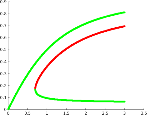
It shows in addition that while the first and second of these steady states are asymptotically stable the third is a saddle with a one-dimensional unstable manifold. A plot of the steady states as a function of the parameter , see Figure 2, suggests that there is a fold bifurcation.
For higher values of it is possible to derive a polynomial equation of degree for . There is no obvious reason why this polynomial should not have an arbitrarily large number of positive roots for arbitrarily large. A simple upper bound is that the polynomial can have no more than positive roots for odd and no more than for even.
In general it is difficult to obtain information about the stability of the steady states by analytic methods. In the case the vector field defining the dynamical system has negative divergence and so by Dulac’s criterion und Poincaré-Bendixson theory all solutions converge to the steady state as . The system can exhibit damped oscillations as will now be shown. To do this we choose parameters so that
| (36) |
For fixed values of the quantities and the quantities and are bounded uniformly in the quantities appearing in (36). Thus if we make and small while fixing the other parameters we can arrange that the left hand side is smaller than the right hand side. If starting from there we make large while fixing the other parameters we can arrange that the left hand side of (36) is greater than the right hand side. It follows that parameter values exist for which (36) holds. The reason why this is interesting is that the discriminant of the characteristic equation of the linearization is the sum of a term which vanishes when (36) holds and the expression . Thus when (36) holds the linearization has eigenvalues with negative real part and non-zero imaginary part and there are damped oscillations.
An interesting limiting case of the agonist-only system is obtained by assuming that and . We refer to this as the kinetic proofreading system since it is closely related to McKeithan’s kinetic proofreading model [11]. In fact McKeithan only considered the case but this makes no essential difference for the analysis which follows. It was observed by Sontag [13] that the deficiency zero theorem of chemical reaction network theory can be applied to McKeithan’s system to conclude that there is a unique steady state in each stoichiometric compatibility class and that this solution is asymptotically stable in its class. Strictly speaking chemical reaction network theory is applied to the extended system which includes free receptors and free ligand as variables. To show that the steady state is globally asymptotically stable it suffices to show that there are no -limit points on the boundary. That this is the case can be proved just as we did for the full system above. The steady state is hyperbolic as follows from Appendix C of [3].
Consider now the full agonist-only system. Setting gives a system where the kinetic proofreading system is coupled to a system describing the decay of . The steady state of the kinetic proofreading system gives rise to a steady state of the agonist-only system with which is on the boundary of the biologically feasible region and is a hyperbolic sink. Denote its coordinates by . For small and positive there exists a hyperbolic sink which is a small perturbation of that for . It must be in the biologically feasible region since there and equation (1) would imply that there if were negative. Thus for sufficiently small values of there exists a positive steady state which is a hyperbolic sink close to . There exists a positive number such that for sufficiently small, say , is the only -limit point of any solution in the open ball of radius about that steady state.
Let be the Lyapunov function in the proof of the deficiency zero theorem. It is known from general arguments that with equality only for . It follows that on the complement of the ball of radius about the steady state the function has a strictly negative maximum. We can consider the behaviour of the function for solutions of the system for positive . For small it is still a Lyapunov function on the complement of a small ball about the steady state while there are no -limit points except the steady state itself within that ball. Hence for sufficiently small a solution can have no -limit points other than the steady state. It follows that for small the steady state is globally asymptotically stable. Of course this means that the limiting system obtained from the agonist-only system by passing to a solution through an -limit point also has a unique steady state which is globally asymptotically stable for sufficiently small. A similar argument applies in the case of the full system (1)-(7) since in that case the system obtained by setting and to zero is just the product of two copies of the corresponding system in the agonist-only case.
4 The response function
This section is concerned with the agonist-only system. From a biological point of view the essential input parameters to the system are the ligand concentration and the binding time of the ligand to the receptor, which in the model corresponds to . The latter is a measure of the signal strength. The essential output is the value of which is a measure of the activation of the T cell. Given values of , and the other parameters we can consider the value of in a steady state. In fact it is more convenient to use the quantities and . This leads to a response function . If there is more than one steady state for a given choice of the parameters this has to be thought of as a multi-valued function. It might naively be thought that should be an increasing function of and a decreasing function of : more antigen leads to more activation of the T cell and a longer binding time leads to more activation. This turns out not to be the case and the function is not a monotone function of its arguments. This was observed in the case of the dependence on in the simulations of [5]. It is possible to understand intuitively how this situation can arise. An increase in the stimulation of the T cell leads to activation of SHP-1 and that in turn has a negative effect on the activation of the T cell. Many of the calculations in this section are guided by those in [5].
The behaviour of the response function will be estimated in various parameter ranges. In order to do this it is useful to parametrize the solutions in a certain manner which will now be described. In the case of a steady state the equation (3) is a linear difference equation for the with constant coefficients. This suggests looking for power-law solutions, an idea which motivates the following result.
Lemma 2 Steady state solutions of equations (2)-(4) in the agonist-only case can be parametrized in the form
| (37) |
where the coefficients and are positive and depend on . The quantities and are given by
| (38) |
and satisfy .
Proof Note first that the quantities in (38) are the roots of the characteristic equation
| (39) |
associated to the difference equation already mentioned and it is obvious that they are positive. The fact that they satisfy the characteristic equation is equivalent to the condition that the defined by (37) satisfy the steady state form of equation (3). That can be seen by noting that the function on the left hand side of (39) is negative at . The condition that the quantities satisfy the equations (2)-(4) with is equivalent to the conditions that they satisfy (37) with as in (38) and certain coefficients and together with the equations obtained by substituting (37) into the equations and . The explicit form of these last equations is
| (40) | |||
| (41) |
It follows from the discussion in Section 3 that , which was denoted there by , is uniquely determined for fixed values of the parameters in and fixed . Thus for fixed values of these parameters and all quantities in (40) and (41) except and are known. It will now be shown that these equations have a unique solution for and . Note that
| (42) |
as can most easily be seen by multiplying out the left hand side of this equation and substituting for and , which are the sum and product of the roots of the characteristic equation (39). Thus equation (41) gives a positive expression for . Note also that (42) implies that the factors in the product on the left hand side of that equation have opposite signs. Since the first factor is positive and the second negative. Substituting the expression for into (40) gives an equation of the form
| (43) |
whose right hand side is positive. Here
| (44) | |||
| (45) |
It follows from the fact that the first factor on the left hand side of (42) is positive that the first factor in the expression for is negative and hence that itself is positive. In addition, a straightforward computation shows that . If were not positive then the quantity in square brackets on the left hand side of (43) would be positive. If is positive then the fact that implies that the quantity in square brackets is again positive. Hence in any case (43) can be solved to give a unique positive value of . Then can be determined in such a way that (40) and (41) hold. This completes the proof of Lemma 2.
Lemma 2 shows that for fixed parameters in (2)-(4) and a fixed value of the steady state values of all the are determined but this does not yet give expressions for the which can be directly applied to study the properties of the response function. For the purposes of what follows it is convenient to rewrite (8) in the form
| (46) |
The equation for can be solved to give the relation with . Summing the expression for given in Lemma 2 over gives
| (47) |
The following equation relating and is equation (21) of [5].
| (48) |
Combining the last two equations gives
| (49) |
Having completed the necessary preliminaries we now proceed to study the qualitative behaviour of the reponse function in different regimes. When is small it is to be expected that the concentration of the phosphatase is small and that the response function resembles that of the kinetic proofreading model. It will now be shown that when is small the leading term in the function depends linearly on with slope one and the additive constant in this linear function will be determined. The equation (46) can be written in the form
| (50) |
Note that so that this equation implies that
| (51) |
where . Using (48) it is possible to write down an explicit expression for , namely
| (52) |
It follows from (49) that
| (53) |
Combining these equations gives
| (54) |
The function of and in this equation defines a function of . This function of tends to a positive limiting value as . Now and . Hence for fixed we can replace the function of and in the above expression by its limiting value for . If the resulting relation is plotted logarithmically it gives a straight line of slope one as the leading order approximation in the limit .
Next we look at an intermediate regime where the amount of activated SHP-1 is well away from both zero and . As a first step, we obtain an estimate for which is sharper than that in Lemma 2. To do this we compute the left hand side of the characteristic equation (39) for . The result is . It follows that . Hence . Substituting this into (49) gives . Note that . Hence a positive lower bound for implies a positive lower bound for .
Next we will derive a lower bound for in the case that is large. This will be proved by contradiction. Suppose that for some . Then it follows from the characteristic equation that . Using this in the equation for gives . It follows that
| (55) |
It is then clear that for a given value of and fixed values of the parameters other than this leads to a contradiction if is sufficiently large. In other words, given any there is a lower bound for which implies that . It is convenient to make the restrictions that and since then it is possible to replace in (55) by by using (51).
From (38) it can be concluded that
| (56) | |||
| (57) |
where . This gives approximate expressions for the roots of the characteristic equation if is small. As a consequence of these equations
| (58) |
Taking the expression for supplied by Lemma 2 and using (48), (49) and (51) gives
| (59) |
This implies that and the expression relating and then shows that . In fact
| (60) |
These relations indicate that in leading order is proportional to . However it is also the case that
| (61) |
which indicates that in leading order is proportional to . Hence
| (62) |
and
| (63) |
where . Combining these two relations gives
| (64) |
Substituting this back into the equation for gives
| (65) |
This means that
| (66) |
where . Choosing small enough makes small. With fixed, making large enough makes small. Thus can be made as small as desired by choosing sufficiently small and sufficiently large.
Theorem 2 Consider the response function for the steady states of the system (1)-(4) with and . Choose fixed values for all parameters in the system except and . Suppose that . Let . Then there exists a constant with such that the following holds. If there exists such that if the inequality
| (67) |
holds on the interval .
Proof To obtain the conclusion of the theorem it suffices to show that under the given assumptions can be made as small as desired. That this is possible follows from the discussion above.
Note that this theorem implies, in particular, that for and suitable values of and there exists a range of in which the response function is decreasing. The theorem also implies that in this regime the reponse function can be an increasing function of . This effect was not captured by the calculations of [5] since there was assumed to be so small as to be negligible.
Finally we examine the regime where is small but the phosphatase is close to being completely activated. This means that is close to one. This holds provided is sufficiently large compared to . It remains to check that such a regime actually occurs for some values of the parameters. It is possible to make large while keeping constant. This can be done by making large. This makes large without making small. Hence it makes large and hence close to . In this regime the function of and occurring in the expression for can be replaced by its limit for and we again get a region where the slope of the graph of as a function is one but the line has been shifted compared to that obtained for small.
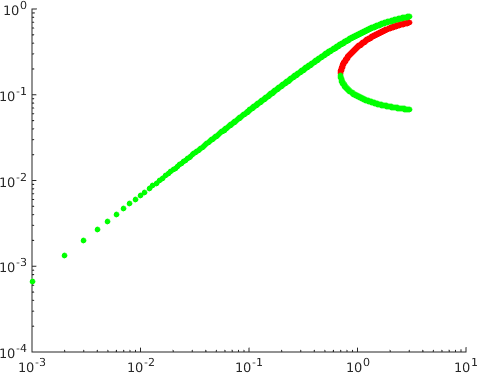
In [5] these types of behaviour were exhibited numerically in the case with biologically reasonable choices of the parameters. We found that changing these parameters a little allows similar observations to be made in the case . In the plot shown in Figure 3
the three regimes can be seen together with a fourth regime where is no longer small. It is clear that a regime of this type must exist since the response function is globally bounded.
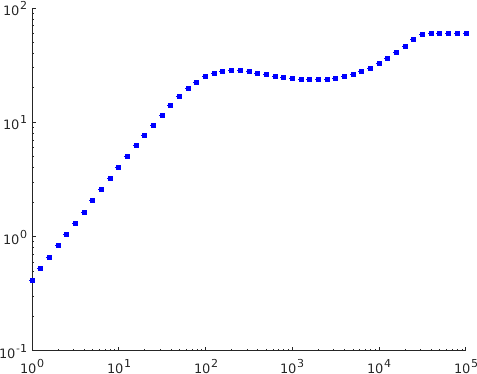
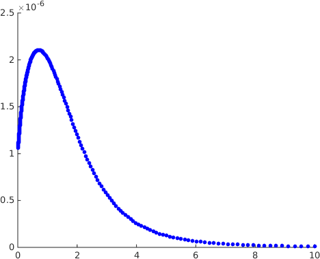
We now turn to the dependence of the response function on . It has been suggested in [9] that the kinetic proofreading model with negative feedback as studied here is not able to explain the presence of an optimal dissociation time, a biological effect confirmed by the experimental work of [10]. The plots of the response as a function of the dissociation time in that type of model in [9] show that it is increasing. Having an optimal dissociation time would require that there be a region where this function is decreasing. The response function being increasing as a function of the dissociation time corresponds to its being decreasing a function of . Here we have given an analytical proof in Theorem 2 that there exist parameters for which the response is an increasing function of , in contrast to the plots in [9]. Since the theorem is of limited help in finding explicit parameters for which this happens we also did a numerical search and identified parameters of this type. The results are displayed in Figure 4, where it is seen that has a maximum as a function of for fixed , which corresponds to an optimal dissociation time.
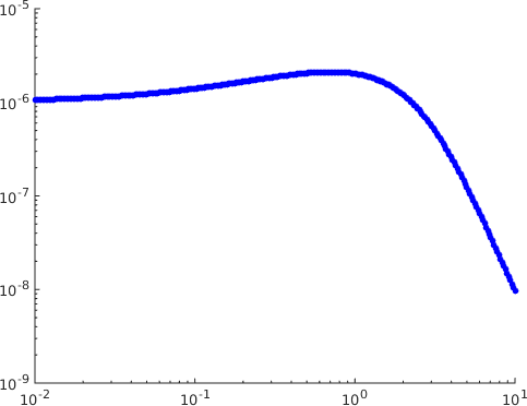
The conclusion of both the analytical and the numerical work is as follows. The claim that the kinetic proofreading model with feedback can only produce a response which is a decreasing function of the parameter is dependent on the parameter values chosen to do the simulations and not a general property of the model.
5 Including the antagonist
When the antagonist is included the output variable expressing the degree of activation of the T cell is . Now asymptotic expressions for this quantity will be derived. It has already been shown that for a steady state of the system (1)-(7) the quantities and can be expressed in terms of the parameters. The equation for can be solved to give the relation . solves the same difference equation as in the agonist-only case and solves the difference equation obtained from that one by replacing by . The quantities , , and differ in the two cases. We can nevertheless proceed as in the former case to see that the solutions for and allow parametrizations in terms of these quantities as before. Note that using the equations (8) and (9) it is possible to eliminate the from the equation for and the from the equation for . Thus we have coupled equations for the and which can be analysed just as in the agonist-only case to express and as functions of and the parameters. We can also write and as functions of and respectively. Proceeding as in the agonist-only case we get an expression for in the kinetic proofreading regime. The multiple of obtained there as leading term is replaced by a linear combination of and .
Next the intermediate regime will be considered. For this it is necessary to define a new parameter . There are asymptotic expressions for and where the leading terms are just as in the agonist-only case. In particular they are the same for and . Two asymptotic expressions for the quantity can be obtained.
| (68) | |||
| (69) |
This gives an expression for in terms of . As in the agonist-only case this gives an expression for where the dependence on has been eliminated in leading order.
| (70) |
where is defined in terms of as in the agonist-only case. Following the steps used in the agonist-only case leads to an expression for which is the same as that previously obtained for except that the expression is replaced by . This leads in the end to an asymptotic expression for under a suitable assumption and . The assumption made in the agonist-only case can naturally be written as an assumption on and in the present case it is replaced by an assumption on . This implies that under certain circumstances increases when increases and is held fixed. An increase in the amount of self-antigen can lead to a decrease in the response to a foreign antigen.
6 Conclusions and outlook
In this paper some properties of the solutions of the model of [5] for T cell activation were proved. A new discovery was that already in the case of three phosphorylation sites () there can exist more than one positive steady state for given values of the parameters. Another new observation is that damped oscillations can occur. It was also proved that, as suggested by the calculations in [5], the output variable (concentration of the maximally phosphorylated receptor) is a decreasing function of the concentration of antigen in some parts of parameter space. In an analogous way it was proved that under some circumstances the activation in response to an agonist can be decreased by increasing the concentration of the antagonist. It was proved that it can also happen that is an increasing function of the dissociation constant . This abstract result was given a concrete illustration by a plot showing that can have a local maximum as a function of .
The stability of the steady states was only determined analytically in the very special cases and close to zero. For numerical calculations showed the occurrence of two stable steady states for certain values of the parameters. It was proved that damped oscillations occur but can there also be sustained oscillations (periodic solutions)? It is thus clear that there remain several aspects of the dynamics of this system which would profit from further investigations, analytical and numerical.
In immunology it is important to describe diverse situations including the course of different types of infectious disease, the development of autoimmune diseases and the destruction of tumour cells by the immune system. It would be unreasonable to expect that a simple mechanism could be the key to describing all these situations. One strategy to try to obtain more understanding is to choose one mechanism and to investigate which types of situations it suffices to describe. This may be done by combining mathematical models with experimental data. What are the restrictions under which the type of model studied in this paper might be appropriate? The first assumption is that in the situation to be explained the distinction between self and non-self takes place within an individual T cell. In other words it is assumed that it is not necessary to consider the population dynamics of the T cells involved or even the interaction of their population with that of other types of immune cells such as regulatory T cells or dendritic cells. A quite different type of mathematical model, where population effects are considered, can be found in [14]. In that case, in contrast to the lifetime dogma, the response depends on the rate of change of the antigen concentration. The second assumption which is important for the models studied here is that the distinction between self and non-self takes place on a sufficiently short time scale, say three minutes. On longer time scales there may be essential effects related to the spatial distribution of molecules on the T cell surface (formation of the immunological synapse) so that a description by means of ordinary differential equations may be insufficient. It may also happen that some T cell receptors become inactive on a longer time scale (limiting signalling model, cf. [10]).
In this paper we have concentrated on studying the mathematical properties of a particular model for the biological phenomenon of T cell activation with arbitrary values of the parameters. A complementary question is to what extent known experimental data on the parameters may further constrain the dynamics in this model. In addition it is important to know whether this model is consistent with all biological data and how it compares to other possible models for the same biological system. For a discussion of this we refer to [9], [6] and [10]. It was indicated in [10] that the situation where is a decreasing function of cannot be reproduced using the model of [5]. Our results indicate that a failure of the model to reproduce this effect must depend not only on the model itself but on the choice of parameters used for simulations. At the same time it may be that this effect only occurs in experiments where the measurements are done on long time scales (many hours) and not on the time scale of the initial activation (a few minutes) for which the models of [1] and [5] were primarily intended. We plan to investigate these questions further elsewhere.
References
- [1] Altan-Bonnet, G. and Germain, R. N. 2005 Modelling T cell antigen discrimination based on feedback control of digital ERK responses. PLoS Biol. 3(11), e356.
- [2] Butler, G. and Waltman, P. 1986 Persistence in dynamical systems. J. Diff. Eq. 63, 255–262.
- [3] Feinberg, M. 1995 The existence and uniqueness of steady states for a class of chemical reaction networks. Arch. Rat. Mech. Anal. 132, 311–370.
- [4] Feinerman, O., Germain, R. N. and Altan-Bonnet, G. 2008 Quantitative challenges in understanding ligand discrimination by T cells. Mol. Immunol. 45, 619-631.
- [5] François, P., Voisinne, G., Siggia, E. D., Altan-Bonnet, G. and Vergassola, M. 2013 Phenotypic model for early T-cell activation displaying sensitivity, specificity and antagonism. Proc. Nat. Acad. Sci. (USA) 110, E888–E897.
- [6] François, P., Hemery, M., Johnson, K. A. and Saunders, L. N. 2015 Phenotypic spandrel: absolute discrimination and ligand antagonism. Phys. Biol. 13, 066011.
- [7] Hale, J. K. 2009 Ordinary Differential Equations. Dover, Mineola.
- [8] Hirsch, M. and Smith. H. 2005 Monotone dynamical systems. In Canada, A., Drabek, P. and Fonda, A. (eds.) Handbook of Differential Equations, Ordinary Differential Equations 239–357.
- [9] Lever, M., Maini, P. K., van der Merwe, P. A. and Dushek, O. 2014 Phenotypic models of T cell activation. Nature Reviews Immunology 14, 619–629.
- [10] Lever, M., Lim, H. S., Kruger, P., Nguyen, J., Trendel, N., Abu-Shah, E., Maini, P. K., van der Merwe, P. A. and Dushek, O. 2016 Architecture of a minimal signaling pathway explains the T-cell response to a million-fold variation in antigen affinity and dose. Proc. Natl. Acad. Sci. USA 113, E6630–E6638.
- [11] McKeithan, T. W. 1995 Kinetic proofreading in T-cell receptor signal transduction. Proc. Nat. Acad. Sci. (USA) 92:5042–5046
- [12] Murphy, K. 2012 Janeway’s Immunobiology, 8th Edition. Garland Science, New York.
- [13] Sontag, E. D. 2001 Structure and stability of certain chemical networks and applications to the kinetic proofreading model of T-cell receptor signal transduction. IEEE Trans. Aut. Control 46, 1028–1047.
- [14] Sontag, E. D. 2017 A dynamical model of immune responses to antigen presentation predicts different regions of tumor or pathogen elimination. Cell Systems 4:231–241.