Multiplexing in Networks and Diffusion
Abstract.
Social and economic networks are often multiplexed, meaning that people are connected by different types of relationships—such as borrowing goods and giving advice. We make three contributions to the study of multiplexing. First, we document empirical multiplexing patterns in Indian village data: relationships such as socializing, advising, helping, and lending are correlated but distinct, while commonly used proxies for networks based on ethnicity and geography are nearly uncorrelated with actual relationships. Second, we examine how these layers and their overlap affect information diffusion in a field experiment. The advice network is the best predictor of diffusion, but combining layers improves predictions further. Villages with greater overlap between layers (more multiplexing) experience less overall diffusion. This leads to our third contribution: developing a model and theoretical results about diffusion in multiplex networks. Multiplexing slows the spread of simple contagions, such as diseases or basic information, but can either impede or enhance the spread of complex contagions, such as new technologies, depending on their virality. Finally, we identify differences in multiplexing by gender and connectedness. These have implications for inequality in diffusion-mediated outcomes such as access to information and adherence to norms.
Keywords: networks, social networks, multiplex, multi-layer, diffusion, contagion, complex contagion
JEL codes: D85, D13, L14, O12, Z13
1. Introduction
People maintain many different types of relationships—for example, collaborating with colleagues at work, relying on friends and acquaintances for assistance and advice, and engaging in the borrowing and lending of money or goods with family and friends. A given pair of people can have multiple such relationships. For example, college students’ partners in social activities overlap with, but also differ from, the people to whom they turn during times of stress or for academic collaboration (Morelli et al., 2017; Jackson et al., 2024).
The coexistence of distinct types of relationships among the same population is known as multiplexing (see, e.g., Kivela et al. (2014)), and the interdependence of different types of relationships has been discussed since Simmel (1908). Although numerous case studies have examined multiple relationships, many basic questions remain open concerning the patterns of multiplexing in social and economic relationships, as well as how multiplexing impacts outcomes of interest such as information diffusion.
In this paper, we make three contributions.
First, in Section 2, we perform unsupervised statistical analyses on correlation structures across network layers in two large datasets. We document both significant correlation between different network layers (types of relationships) and meaningful differences in their patterns. We show that layers of informational relationships, financial relationships, and social relationships, among others, exhibit strong correlations in a sample of 143 villages in Karnataka, India, comprising nearly 30,000 households (Banerjee et al., 2013, 2019; Banerjee et al., 2024b). At the same time, different layers display distinct patterns and differ in density and other network statistics. We also show that proxies for social relationships that are commonly used in the peer effects literature, such as geographic proximity or co-ethnicity (in our data, being members of the same jati, or subcaste), are nearly orthogonal to the other layers. This suggests that relational variables constructed based on geographic or ethnic covariates can fail to serve as accurate surrogates for actual social and economic relationships.
Second, we use supervised statistical methods to show that distinctions among layers are substantively important for the study of economic outcomes, specifically the diffusion of information or behaviors. While one might have expected little difference in the predictive power of different network layers for outcomes of interest, we find that the different layers contain distinct information and combine to form a nuanced overall picture. Using data from a randomized controlled trial of information diffusion, we show that some layers are more predictive of diffusion than others—with an “advice” layer standing out—and moreover that using a suitable combination of layers yields predictions significantly better than those based on any single elicited layer. A combination of layers also affords better predictions than using the union or intersection of layers. These findings indicate that the elicited layers are not simply noisy observations of a latent one-dimensional relationship, instead containing information richer than any one-dimensional summary. Without properly accounting for the multiplexed nature of relationships, researchers may arrive at misleading conclusions about peer effects and influence.
An additional finding regarding ethnic links further supports the point that links are most usefully viewed as multi-dimensional. We show that, while the jati layer is the least predictive of diffusion and not a good proxy for actual relationships, combining it with other layers significantly improves diffusion predictions. Thus, although jati is not a good substitute for elicited network data,111As we discuss below, using the jati variable drastically over-predicts links within jati, and under-predicts them across jati. One conjecture as to why the jati layer helps in predicting diffusion is that patterns of information passing on the network are related to jati. it can serve as a valuable complement.
We close Section 2 with an important and novel empirical observation: villages that are more multiplexed (have more strongly correlated layers) experience less diffusion. This correlation between layer overlap and diffusion sets the stage for our theoretical analysis.
Motivated by the fact just presented, in Section 3 we develop our third main contribution—a new model of and theoretical results on how multiplexing relates to diffusion. First, we model how the degree of multiplexing affects a standard diffusion or contagion process in which a person may be infected/informed by any single infected other (called simple contagion). We introduce a definition capturing what it means for an individual to be unambiguously more multiplexed in one multiplex network than another. When such a comparison can be made, we prove that the more multiplexed individual is less likely to become infected for any given probability of neighbor infection. Building on this result, we demonstrate that in a standard SIS (Susceptible-Infected-Susceptible) simple contagion model, the steady-state infection rate decreases as individuals become more multiplexed. These results can be summarized by saying that multiplexing impedes simple diffusions. We then develop a theory of how multiplexing impacts complex diffusion processes—ones in which people only become infected or adopt a new behavior/practice if they experience sufficiently many interactions with infected others. Here we show that multiplexing can either enhance or impede diffusion, depending on the virality of the process. The nonmonotonicities identified by our theory reveal that multiplexing has subtle implications for threshold contagion models.
We close the paper in Section 4 with observations about how multiplexing varies with individual characteristics and some implications for issues of inequality. We find that women’s networks display significantly more multiplexing than men’s networks, and that multiplexing correlates negatively with the number of connections a person has. Given our theoretical and empirical evidence showing how multiplexing can impede simple diffusions, this suggests that multiplexing could function as a channel limiting women’s exposure to information. More broadly, demographic differences in multiplexing imply that network-mediated contagions work differently in different subpopulations—a rich topic that we believe deserves further study.
The literature on multiplex networks has begun to grow in the last decade (Contractor et al., 2011; Boccaletti et al., 2014; Kivela et al., 2014; Dickison et al., 2016; Bianconi, 2018). The recognition that people are involved in different types of relationships dates to some of the original works on network analysis (e.g., Simmel (1908)), and instances of the fact that different layers can serve different roles have been analyzed over time (Wasserman and Faust, 1994; Becker et al., 2020). More recent studies have shown that distinguishing between different networks and tracking their interplay can be important in understanding cooperative behavior (Atkisson et al., 2019; Cheng et al., 2021) as well as understanding play in network games and targeting policies to influence it (Walsh, 2019; Zenou and Zhou, 2024).
Our contributions to the literature on multiplex networks are threefold.
First, we provide some of the first detailed statistical analyses of how multiple layers relate to each other in empirical social networks. Second, we show how different layers—as well as the level of correlation between layers—predict diffusion outcomes. This suggests that unidimensional theories of diffusion and contagion can miss important factors that determine the extent of diffusion. Third, we introduce a model and develop a new theoretical analysis of how correlation between layers impacts diffusion, which provides a basis for interpreting our empirical observations about multiplexing and diffusion.
While some theoretical work has examined simple (Hu et al., 2013; Larson and Rodriguez, 2023) and complex (Yağan and Gligor, 2012; Zhu et al., 2019; Kobayashi and Onaga, 2023) diffusion on multiplexed networks, previous analyses have focused on independently distributed layers. Such diffusion models are a more direct extension of diffusion on one layer and the proofs in the existing literature leverage that fact. Our analysis examines how changes in layer overlap affect diffusion. In addition—and in contrast to prior models—our model also allows for interactions (such as conversations or information transmissions) to be correlated across layers, even conditional on links.
Our findings on the impact of multiplexing on diffusion can help inform a nascent and important literature on the incentives to form multiplexed networks (Billand et al., 2023; San Román, 2024). For example, a series of empirical studies on rural developing economies emphasize the role social networks play in risk-sharing arrangements (Townsend, 1994; Fafchamps and Gubert, 2007; Ambrus et al., 2014). This raises a fundamental question: If individuals primarily organize their relationships around risk-sharing and multiplex other relationships on top of the risk-sharing relationships, how might these structures affect the diffusion of new information or technologies? Both our empirical findings and theoretical results shed light on this issue.
2. Multiplexing in the Data
2.1. Two Data Sets
We study two different data sets of multiplex networks in a total of 143 villages, both from the state of Karnataka, India, covering a total population of nearly 30,000 households.
2.1.1. The Microfinance Village Sample
The first dataset that we use, which we refer to as the “microfinance village sample,” comes from network data collected in Wave II of a study of 75 villages (Banerjee et al., 2013; Banerjee et al., 2024b). In 2012, that study obtained a complete census of the 16,476 households across these 75 villages. From 89.14% of these households, it then collected detailed socio-economic network data, described below. (This means that the study obtained information on 98.8% of the links.222Given our focus on undirected graphs, we elicit a link as long as at least one of the two households on either end is sampled. With 89.14% of the households being sampled, for two arbitrary nodes and , we compute P( or in sample) = .)
The researchers collected information on various types of interactions for each respondent, spanning social, financial, informational, kinship, and religious networks. The surveys asked respondents about the following types of relationships, each listed with an abbreviated label that we use from now on to refer to it:
-
(1)
social: to whose home does the respondent go and who comes to their home, as well as which close relatives live outside their household;
-
(2)
kerorice: from whom does the respondent borrow kerosene/rice and to whom does the respondent lend these goods;
-
(3)
advice: to whom does the respondent give information/advice;
-
(4)
decision help: to whom does the respondent turn for help with an important decision;
-
(5)
money: if the respondent suddenly needed to borrow 50 rupees for a day, to whom would they turn, and who would come to them with such a request;
-
(6)
temple: if the respondent goes to a temple, church, or mosque, who might accompany them;
-
(7)
medic: if the respondent had a medical emergency alone at home, whom would they ask for help in getting to a hospital.
Additionally, we have information on the jati (subcaste) and GPS coordinates for each household. This allows us to construct jati networks (in which pairs from the same subcaste are linked) and geographic networks, whose edges are labeled by distance in physical space. Variables of these types have been used as proxies for social networks in prior studies (e.g., Sacerdote, 2001; Fafchamps and Gubert, 2007; Munshi and Rosenzweig, 2009).
2.1.2. The Diffusion RCT Sample
The second dataset that we use, which we call the “RCT village sample,” contains multiple network layers from a set of 68 different villages collected by Banerjee et al. (2019).
The network data was collected in a manner similar to that of the Microfinance Village Sample. The surveys elicited information about the following layers:
-
(1)
social: to whose home does the respondent go and who comes to their home to socialize;
-
(2)
kerorice: from whom does the respondent borrow kerosene/rice or small amounts of money and to whom does the respondent lend these goods;
-
(3)
advice: to whom does the respondent give information/advice;
-
(4)
decision: to whom does the respondent turn for help with an important decision?
While we have jati information for the RCT villages, we lack GPS data for this sample.
In addition, we have the data from a randomized controlled trial (RCT) studying diffusion in these villages, which is the subject of Banerjee et al. (2019). This RCT provides cleanly identified estimates of diffusion, allowing us to examine how diffusion varies with different aspects of multiplexed networks. Specifically, in each village either 3 or 5 individuals (determined uniformly at random) were seeded with information about a promotion. Villagers could obtain a non-rivalrous chance to win either cash prizes or a mobile phone by calling in to register for the promotion.333In particular, they had to dial the provided promotional number and leave a “missed call.” This was a call that we registered but did not answer and was free for the participant to make, which was a standard technique for registration at the time. Registered callers were visited a few weeks later and received a reward.444The individual rolled a pair of dice and received INR 25 the number rolled. This yielded cash prizes of amounts ranging from INR 50 (for a 2) to INR 275 (for an 11). A roll of 12 was rewarded with a cell phone worth INR 3000. The expected value of the prize was INR 255, which was more than half of a day’s wage in the area. Thus, the experiment induced the diffusion of a non-rivalrous, valuable piece of information. The outcome variable of interest is the number of households that registered. There was exogenously randomized variation in the position of the random seeds in the network, and more central seeds caused larger diffusions. We use our data on multiplexing to examine how diffusion depends on the network statistics of the seeds in various network layers, used individually and in combination, and on network multiplexing levels.
2.2. The Layers and Multiplexing Patterns
We begin with some descriptive statistics on the network layers. A link is present in a given layer if either household named the other household in one of the questions in that category (e.g., we code a kerorice link if either household reports borrowing kerosene or rice from or lending it to the other household). In terms of notation, we define a multi-layered, undirected network for each village ,555One can also define directed networks from our data, which we comment on at several points below. Directed links open some important but tangential questions for multiplexing, which we leave for further research. for layer , with if either household or reported having a relationship of type . We add another layer where and are linked if they belong to the same jati. For the Microfinance Village Sample, where GPS data are available, we construct a weighted graph where the entry is the geographic distance between the two households.
The union layer has a link present if a link exists in any layer. The intersection layer has a link present if it exists in all layers.666Both of these definitions include the jati layer but exclude geography, since we are able to define the geographic layer for only one of our datasets, and it is a weighted network in any case. We make these definitions to maintain consistency of the meaning of the union and intersection layers across the two data sets.
We also build a weighted and directed network whose edge weights are the sums of indicators for links in all directed layers (thus excluding jati and geography). We call this the total network. Finally, below we describe another weighted and directed aggregate network that we build from the principal component analysis.
2.2.1. Descriptive Statistics
| Network | degree | degree S.D. | density | triangles | clustering |
|---|---|---|---|---|---|
| Microfinance villages | |||||
| social | 15.296 | 7.841 | 0.079 | 2635.040 | 0.252 |
| kerorice | 7.029 | 3.834 | 0.037 | 594.160 | 0.259 |
| advice | 6.158 | 3.835 | 0.032 | 299.120 | 0.168 |
| decision | 6.553 | 4.309 | 0.034 | 356.040 | 0.169 |
| money | 8.512 | 5.036 | 0.044 | 681.960 | 0.193 |
| temple | 1.709 | 1.899 | 0.009 | 52.040 | 0.175 |
| medic | 6.530 | 3.911 | 0.034 | 369.400 | 0.188 |
| union link | 75.428 | 32.542 | 0.368 | 314121.027 | 0.862 |
| intersect link | 0.576 | 0.883 | 0.003 | 7.000 | 0.203 |
| jati | 68.291 | 34.293 | 0.332 | 310150.907 | 1.000 |
| RCT villages | |||||
| social | 5.711 | 3.626 | 0.031 | 251.271 | 0.185 |
| kerorice | 4.910 | 3.235 | 0.027 | 176.557 | 0.174 |
| advice | 4.197 | 3.091 | 0.023 | 124.100 | 0.161 |
| decision | 4.206 | 3.675 | 0.023 | 125.571 | 0.145 |
| union link | 55.756 | 27.861 | 0.296 | 150771.400 | 0.913 |
| intersect link | 1.812 | 1.829 | 0.010 | 38.871 | 0.229 |
| jati | 52.633 | 28.599 | 0.279 | 150117.500 | 1.000 |
Our first look at the data focuses on basic descriptive statistics, presented in Table 1. The different layers exhibit significantly different patterns of connection. For example, in both datasets, the social layer is denser than the other layers and has among the highest levels of clustering. We observe a higher variance of node degrees in the decision layer than in other comparable layers (e.g., advice).777In the RCT villages the social layer is significantly denser than kerorice, advice, or decision layers (p-values , , and respectively). The advice layer has significantly less variance (p-value ) and more clustering (p-value ) than the decision layer. Similar patterns hold in the Microfinance villages.
We also observe that the microfinance villages and RCT villages differ from each other in some descriptive statistics. Microfinance villages across all network layers are denser on average and exhibit higher levels of clustering, as can be seen in Table 1. The two samples also slightly differ in terms of village size. RCT villages have 197 households on average, while microfinance villages are larger with 216 households on average.
Additionally, the jati layer has by far the highest degree. This finding foreshadows that jati match serves as a poor proxy for other types of relationships, being too dense, too clustered, and too homophilous to predict the other layers.
2.2.2. Correlations among Layers
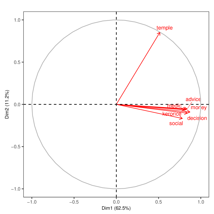
Next, we examine the correlation among layers, pictured in Figure 1.
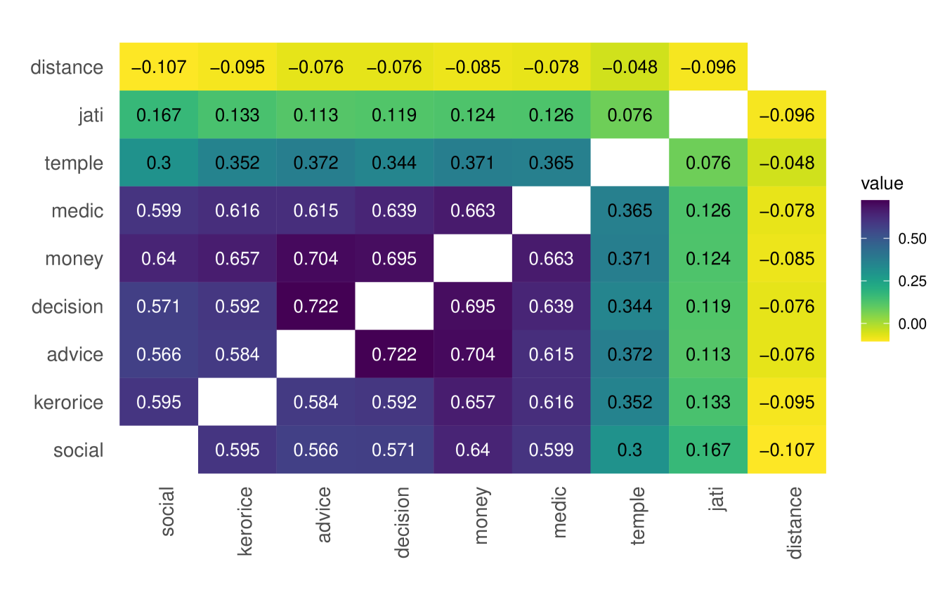
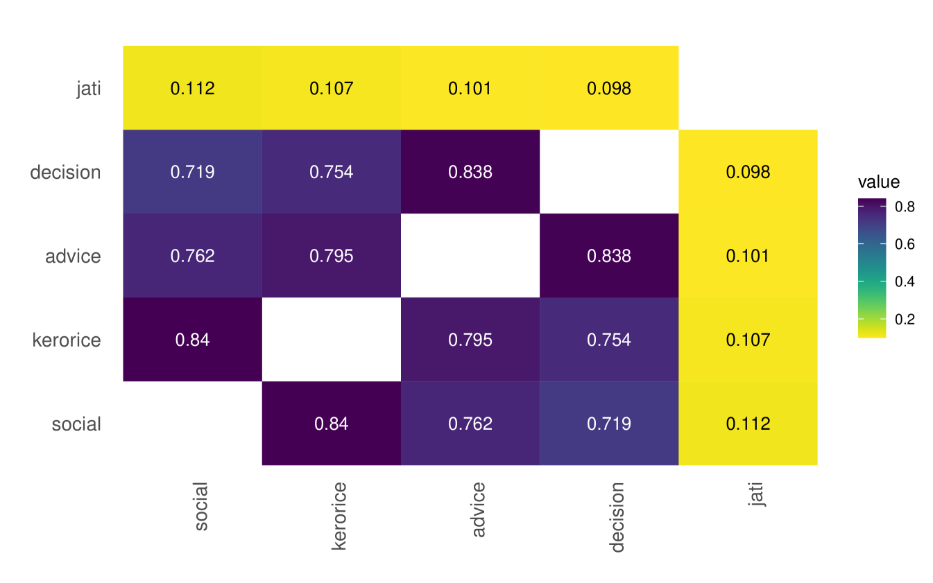
Figure 1 reveals several patterns. First, there are consistently high correlations between layers in both data sets—above 0.5 for most layer pairs. Second, the exceptions are the distance, jati, and temple layers. The jati and distance layers are almost uncorrelated with the other layers,888This does not mean, for instance, that there is not substantial jati-based homophily in these data. The low correlation comes from the fact that the jati layer dramatically over-predicts relationships compared to other layers, so it has many 1’s where there are 0’s in the other layers.,999Distance is higher when people live far from each other and are thus less likely to be linked, all else held equal; this explains the negative signs. while the temple layer has an intermediate level of correlation with others. Third, the layers are more highly correlated in the RCT villages compared to the microfinance villages.
2.2.3. Principal Component Analyses
Our third look at the structure of the networks uses principal component analyses, conducted in two stages.
First, we perform a principal component analysis with all of the layers (excluding the synthetic union and intersection layers). We treat each pair of households (in a given village) as an observation, yielding observations, where is the number of households in village , and the number of dimensions is the number of layers in the given sample.
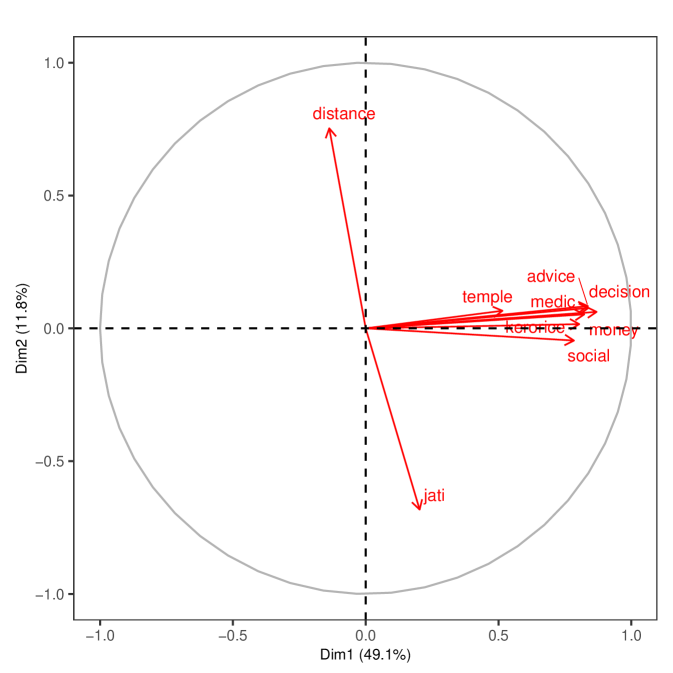
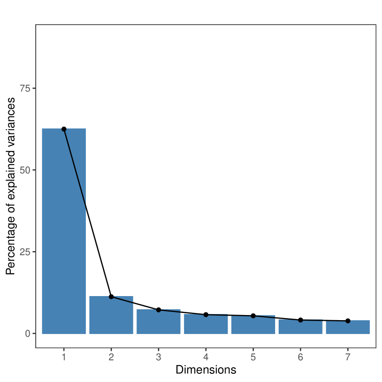
As we see in Figure 2, when including all layers, the first principal component aligns with most relationship layers, capturing almost half (48.7%) of the variation in the microfinance villages and more than two-thirds (72.1%) in the RCT villages. Panels A and B plot the coordinates of the first and second component entries for each link type. Interestingly, jati largely aligns with the second principal component, as one would expect given its relatively low correlation with the other layers. The geographic distance layer is nearly opposite to jati, which reflects the fact that people from the same jati live in close proximity. The complete results appear in Appendix Tables S2 and S3.
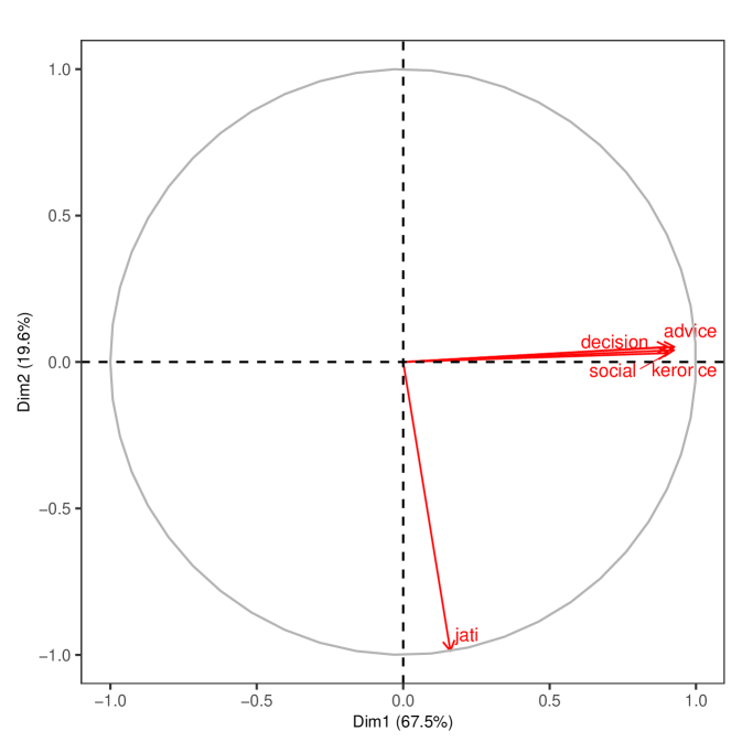
Next, in Figure 3 we repeat the analysis after removing the least correlated dimensions: jati, geography, and temple.101010 We also redo the analysis just dropping jati and geography and keeping temple in Supplemental Appendix Figure S2. Temple is sparse and essentially orthogonal to the other dimensions. This allows us to zoom in on the correlation patterns among the social and economic layers.
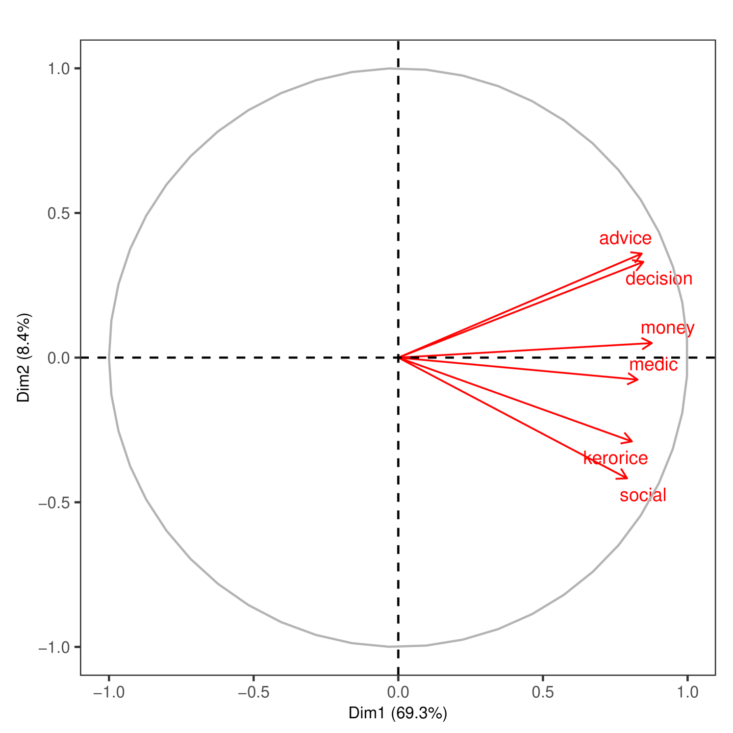
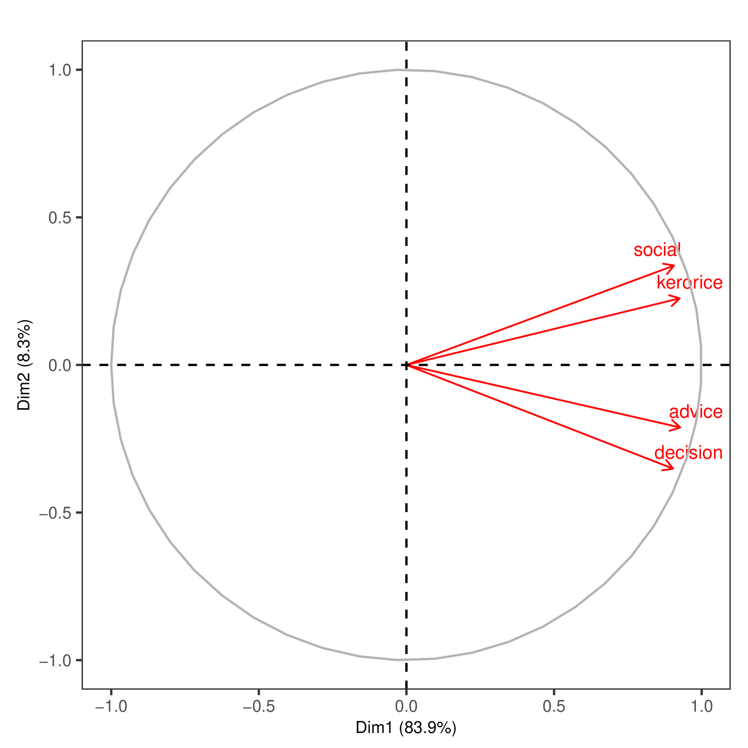
Figure 3 displays the relationship between the layers where we again project them on the first two principal components. In Panel A, we can see three distinct groupings of similar layers in the microfinance villages (advice-decision, money-medic, and kerorice-social). In Panel B, there appear to be two distinct groupings in the RCT villages (advice-decision, kerorice-social), with the first component now explaining 70% and 83% of the variance across the two samples, respectively.
Building the Backbone.
To capture the correlation structure of the network layers, we use the principal component analysis to construct an aggregate network from the multigraph, which we call the backbone. The backbone network is built using the first principal components, constructed as described above. The we use is determined by a so-called ladle plot, with the goal of selecting a cutoff yielding an “optimal” low-dimensional representation (see Luo and Li (2016) for details).111111To select the optimal number of principal components the literature usually relied on a cutoff based on patterns of either decreasing eigenvalues or increasing variability of eigenvectors. Luo and Li (2016) combine these two approaches to better estimate the optimal K. They propose a new estimator, called the “ladle estimator” which minimizes an objective function that incorporates both the magnitude of eigenvalues and the bootstrap variability of eigenvectors. This approach exploits the pattern that when eigenvalues are close together, their corresponding eigenvectors tend to vary greatly, and when eigenvalues are far apart, the eigenvector variability tends to be small. By leveraging both sources of information, the ladle estimator can more precisely determine the rank of the matrix, and thus the optimal number of components to retain.
For a pair in village , we compute the weighted sum of its projections on the first principal components as
In this formula, is the eigenvector associated with the principal component, and the weights are determined by the relative magnitudes of the eigenvalues associated with each component:
For each village , we then define a “backbone” network, , from the principal components as a weighted graph where
In words, the backbone reduces the multiplex data to a synthetic structure by projecting the multidimensional links onto the top principal components. After determining the number of components , we compute each dyad’s coordinates along these components, scaling by eigenvalues, which (as is standard in PCA) quantify the importance of various dimensions. Summing these weighted projections yields a single index.
2.3. Determinants of Diffusion
The empirical analysis demonstrates that multiplexed networks in our data are rich and embed important information that would be lost by collapsing them into a single summary measure. A natural next question is how this distinction between layers matters for outcomes of interest. Here we focus on diffusion in the RCT villages.
We proceed as follows. Based on prior work, we would expect that more central seeds should lead to greater diffusion (Banerjee et al., 2013, 2019). Those papers defined a single network by using the union network and computed diffusion centrality based on that. However, given our rich multiplex data, we note that the seeds’ diffusion centrality differs across layers. Thus, we examine which layer is the most predictive of diffusion in the RCT if we were to compute diffusion centrality based on that layer alone.
We use a specific diffusion centrality measure developed in Banerjee et al. (2013) and further studied in Banerjee et al. (2019). In particular, the diffusion centrality of a node in layer in village , is defined by
where is the number of rounds of communication and is the probability of transmission in each period across any given link. Following Banerjee et al. (2019), for village and network layer , we set , and , where is the largest eigenvalue associated with .121212See Banerjee et al. (2019) for a theoretical foundation for using these as default settings in diffusion centrality. We calculate the diffusion centrality of the seed set of village , , for layer by
We then can calculate how diffusion varies with the diffusion centrality of the randomly assigned seed set under layer by regressing
| (2.1) |
where represents the number of calls received from village (a measure of diffusion of information), and includes controls for number of households, its second and third powers, and number of seeds assigned in that village. We standardize all the regressors.
Table 2 depicts how differently the layers predict diffusion based on our specification in (2.1). (Supplementary Appendix Figure S1 plots the % and % confidence intervals.)
| No. Calls Received | |||||||||
| 1 | 2 | 3 | 4 | 5 | 6 | 7 | 8 | 9 | |
| Social | |||||||||
| () | |||||||||
| [] | |||||||||
| Kero/Rice | |||||||||
| () | |||||||||
| [] | |||||||||
| Advice | |||||||||
| () | |||||||||
| [] | |||||||||
| Decision | |||||||||
| () | |||||||||
| [] | |||||||||
| Jati | |||||||||
| () | |||||||||
| [] | |||||||||
| Union | |||||||||
| () | |||||||||
| [] | |||||||||
| Intersection | |||||||||
| () | |||||||||
| [] | |||||||||
| Backbone | |||||||||
| () | |||||||||
| [] | |||||||||
| Total Links | |||||||||
| () | |||||||||
| [] | |||||||||
| Num.Obs. | |||||||||
| R2 | |||||||||
| Dep Var mean | |||||||||
-
•
Note: Robust standard errors are given in parentheses and p-values in square brackets. Controls added: number of households, its powers, and a dummy for number of seeds in the village. Exogenous variables are the sum of Diffusion Centrality for seeds in each village for the layer. Exogenous variables have been standardized. The total links network is the raw sum of all directed network layers (excluding jati network).
The advice layer stands out as the most predictive, and we see that the kerorice and social layers are also significantly predictive. Notably, consistent with what we observed in the correlations and principal component analysis, jati explains the least of the variation and is not significant.
Interestingly, the four synthetic networks we have mentioned that aggregate the layers in specific ways—union, intersection, total, and backbone—all perform worse than the individual layers with the exception of jati. However, this appears to be rooted in the inclusion of jati in those aggregates. In Supplement A.2 we recreate Table 2 with aggregate layers that omit jati in their construction (this applies only to union, intersection, and backbone). This improves their performance, with the backbone network now yielding an second only to the advice layer.
Given how correlated the layers are, we also perform a LASSO (-penalized) regression to select a sparse set of relevant variables that explain diffusion. We then use post-LASSO least squares to estimate how seed set centrality under the selected layer(s) affects diffusion.
The regression of interest is given by
| (2.2) |
where the variables are as described in (2.1) and instead of running a separate regression for each layer, we now include all the layer variables simultaneously. We are interested in which are estimated to be non-zero and the consistent estimates of these parameters.
A complication we face here is that in order to be consistent, LASSO requires a condition called irrepresentability, which requires the regressors of interest not to be excessively correlated (Zhao and Yu, 2006). In our setting, this requirement fails since the network layers are highly correlated. To overcome this problem, we use the Puffer transformation developed by Rohe (2015) and Jia et al. (2015), which recovers irrepresentability when the number of observations exceeds the number of variables. Although the regressors have correlated columns, by appropriately pre-conditioning the data matrix, we can force its columns to be orthogonal and therefore irrepresentable. Puffer-LASSO then recovers the set of relevant variables with probability tending to one exponentially fast in the number of observations, with consistent parameter estimates, that are asymptotically normally distributed with probability approaching one (Javanmard and Montanari, 2013; Jia et al., 2015; Taylor and Tibshirani, 2015; Lee et al., 2016; Banerjee et al., 2024a).
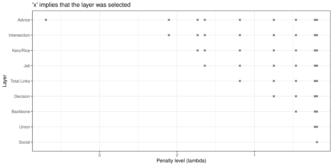
We see the results in Figure 4, where we plot which layers are selected by the LASSO as we increase the penalty level, forcing LASSO to select fewer variables. We find that, at the highest penalty level, only the advice network layer is selected, with the post-puffer LASSO OLS regression in Table 3 depicting a 64% increase in diffusion relative to the mean (). Despite the fact that multiple layers are useful in explaining diffusion, neither the backbone, the union, nor the intersection network proved to be the most useful.
| No. Calls Received | |
|---|---|
| Advice | |
| () | |
| [] | |
| Num.Obs. | |
| R2 | |
| Dep Var mean |
The fact that centrality in the advice layer is singled out as the best predictor of diffusion under sufficiently high penalty does not mean that the other layers have no impact on diffusion. In fact, a combination of the layers still provides significantly more prediction than just the advice layer, as shown in Table 4.
| layer | df | R.sq. | F-stat | p-val | F-stat marginal | p-val marginal |
|---|---|---|---|---|---|---|
| Advice | 1 | 0.233 | 20.057 | 0.000 | ||
| Intersection | 2 | 0.276 | 3.888 | 0.053 | 3.888 | 0.053 |
| Kero/Rice | 3 | 0.281 | 2.134 | 0.127 | 0.415 | 0.522 |
| Jati | 4 | 0.325 | 2.844 | 0.045 | 4.059 | 0.048 |
| Total Links | 5 | 0.343 | 2.602 | 0.044 | 1.771 | 0.188 |
| Decision | 6 | 0.348 | 2.159 | 0.070 | 0.478 | 0.492 |
| Backbone | 7 | 0.353 | 1.851 | 0.104 | 0.416 | 0.521 |
| Union | 8 | 0.353 | 1.564 | 0.164 | 0.021 | 0.884 |
| Social | 9 | 0.353 | 1.349 | 0.238 | 0.026 | 0.873 |
Table 4 presents both cumulative and marginal F-tests as variables are added in the order selected by LASSO. We can see that adding intersection is marginally significant above advice, and further including kerorice and jati yields a more complete model, with an improvement significant at the 5 percent level.131313 In Appendix Table S4 we exclude the extra layers of intersection, union, and backbone, which are “constructed” layers that are derived from these basic layers. F-tests include the basic layers in the order selected by the Lasso. Thus, even though jati serves as a poor substitute for other layers, it turns out to be a useful complement to them in predicting diffusion.
2.4. How the Level of Multiplexing Affects Diffusion
Next, we examine how diffusion depends on the extent to which the layers in a village are multiplexed. Specifically, do villages with greater correlation among their network layers experience higher or lower levels of diffusion? To do this, we first develop a measure of the extent to which a village is multiplexed.
We begin by defining a multiplexing score for household in village as
The multiplexing score for a household measures the average fraction of relationship types it has with each of its neighbors. The numerator calculates the average number of links household has to each neighbor across all relationship types. It does this by first summing the number of links between household and each neighbor across all layers, dividing by the total number of layers , and then summing this average across all neighbors . The denominator counts the number of unique neighbors of household by summing an indicator for whether there is at least one link between and across any layer. For example, if whenever household has a relationship with some other household , then it has all possible relationships with that other household. In contrast, when there is no multiplexing, this measure would be .
We aggregate this to the village level by taking . Further, we define a dummy variable for having an above-median amount of multiplexing in the sample as
Our regression of interest is
| (2.3) |
where denotes the diffusion centrality of the seed set in village for the “advice” layer (which was singled out as the best predictor of diffusion).
Here, captures the returns to increasing the diffusion centrality of the seed set. Since information is seeded in all networks, captures how the extent of diffusion changes with the worst possible seeding (the theoretical intercept). The coefficient captures how incrementally improving seeding differentially affects the extent of diffusion as a function of multiplexing.
The interaction term is particularly important, and its coefficient of primary interest, since villages with low seed set centrality experience very little diffusion, and hence multiplexing has a very limited opportunity to make any difference in diffusion. Thus, multiplexing’s marginal impact (positive or negative) should be most pronounced in settings where the seed set centrality is high.
| Calls per Household | |
|---|---|
| (1) | |
| High Multiplexing | |
| () | |
| [] | |
| Seed Set Centrality | |
| () | |
| [] | |
| High Multiplexing X Seed Set Centrality | |
| () | |
| [] | |
| Num.Obs. |
-
•
Robust standard errors are given in parentheses, while p-values are given in square brackets. Seed Set Centrality comes from the ”advice” layer and has been standardized. Controls for number of seeds and average total degree across network layers have been added.
Table 5 reports the coefficient estimates. As expected, the coefficient on seed set centrality is positive and significant. We also find that both and . Qualitatively, indicates that more multiplexed networks generate less diffusion, with the caveat that these villages could be different for other reasons, and the coefficient is not significant. Importantly, the coefficient indicates that villages with more central seeding—and thus higher levels of diffusion—have their diffusion impeded by multiplexing.
3. A Theory of Diffusion and Multiplexing
We now develop a theory that helps us understand how and why multiplexing affects diffusion. The stylized facts that motivate and structure this theory, established above, are: (i) the network layers are distinct but significantly correlated/multiplexed; (ii) they are differently predictive of diffusion; (iii) multiple layers are predictive of diffusion; and (iv) more multiplexed villages experience less information diffusion.
We approach the problem at two levels. At the individual level, we examine how a node’s probability of becoming infected depends on its multiplexing (for any given probability of infection among neighbors). At the population level, we aggregate the individual effects to analyze broader contagion outcomes. For this population-level analysis, we use the results about individuals as a key lemma in analyzing a canonical SIS contagion process.
We model two rather different types of processes within a common framework. The first is “simple” diffusion/contagion, in which a single contact is sufficient for an individual to become infected. The second is “complex” diffusion, defined as a process in which multiple contacts are needed. We analyze each type in turn, beginning in each case with a result about individual infection probabilities and then aggregating to the societal level.
We begin by outlining our general model of multiplexed diffusion.
3.1. A Model of Diffusion with Multiplexing
We study diffusion/contagion in a society consisting of a finite set of individuals . Each individual has relationships captured via layers , with a generic layer represented by . In each layer , the interactions between individuals are described by a (possibly directed) network with adjacency matrix , such that if there is a link from to in layer (interpreted as being capable of being infected by , e.g., via paying attention to in a model of information flow), and otherwise. We denote the multigraph consisting of layers by .
Let denote the set of layers in which there is a directed link from to . The set of all neighbors for a given node is denoted .
To track infection across time, we index discrete periods by . At each point in time, an individual in the network is in one of two states: Susceptible (S) or Infected (I). The status of individual at time is denoted by the random variable . If , individual is infected at time ; if , individual is susceptible at time . The state of the society at time is given by the vector .
At each time , an individual’s state can change based on the infection status of its neighbors. A susceptible individual becomes infected if it receives at least infection transmissions from its infected neighbors in a given time period. An infected individual recovers (and becomes susceptible again) randomly with a probability at the end of a period. If , this represents a standard (simple) contagion process, while with a threshold this is known as a complex contagion (Granovetter, 1978; Centola, 2010).141414This is closely related to games on networks (Morris, 2000; Jackson and Zenou, 2014).
To complete the description of the model, we examine the mechanics of contagion in more detail. Given that individuals can be connected via multiple layers, we need to define how transmission occurs through multiple layers. Let represent the (random) number of infection transmissions at time to a susceptible node from an infected node , conditional on being infected.151515This is related to the modeling of dosed exposures in the literature on contagion; see Dodds and Watts (2004). At most one transmission can take place per layer. We denote the distribution of infection transmissions from node given by
This is the probability of transmissions; note can capture arbitrary patterns of correlation in infection transmission through multiple layers. For each layer , let be the marginal probability of infection transmission from an infected individual to a susceptible one if they are connected via that layer. We allow different layers to have different contact probabilities, which is needed given the heterogeneity in the roles of different layers discussed in Section 2.3. If there is a positive correlation in transmission across layers, two nodes connected by layers have an infection distribution satisfying .
The probability that a susceptible individual becomes infected at time given the infection status of its neighbors at time is
3.1.1. Comparisons of Multiplexing
Since it is not always possible to order two multigraphs in terms of multiplexing, we define a partial order on the set of multigraphs. We begin with an example illustrating the concept in Figure 5.
In Figure 5(A) we depict a multigraph with 5 nodes and 3 layers. In Figure 5(B), by moving node 1’s link in layer red from node 3 to node 4, we arrive at a graph that is less multiplexed while maintaining the same out-degree. Similarly, in panel C, we again move node 1’s link in layer blue from node 2 to node 5, creating a less multiplexed network as compared to panel B.
To formalize this type of ranking, we define a local multiplexity dominance relation, denoted by . For two multigraphs and , we say —that is is locally less multiplexed than —if can be obtained from by removing a link in some layer between nodes and and adding a new link in that same layer to another neighbor , where ’s connections to occurred in a set of layers that form a strict subset of the layers (except layer ) in which was connected with to start with. This means that: (i) , (ii) and , and (iii) for all other links and coincide.
Given that the local multiplexity dominance relation is acyclic (see Proposition 5 in the appendix), we define the less multiplexed relation, denoted by as the transitive closure of . That is, we say that if there exists a finite sequence of multigraphs such that . The relation forms a partial order on the set of multigraphs.
We now define a corresponding notion for a particular node . We say that if is less multiplexed than (i.e., ) and, moreover, the changes in the network’s multiplexity structure involve node . Formally, holds if and , where denotes the collection of all layers’ adjacency for node . We refer to this refined notion as local multiplexity dominance for node .
3.2. Multiplexing Impedes Simple Diffusion and Contagion
We first analyze the case of simple contagion, . We focus on the case of two layers as this captures all of the essential intuition.
3.2.1. Infection of an Individual
To understand how increasing multiplexing impedes diffusion, it helps to first isolate the comparison on a single pair of links while holding everything else fixed. Specifically, consider some node that is connected in both layers to node in , but in neither layer to another node . Changing from to involves removing one of the layers of ’s connection to and adding it to . Since all other connections of remain unaffected, only events involving the changed links need to be considered to assess the effect on ’s infection probability.
Suppose that both and are independently infected with probability , and similarly for any of ’s other connections. The probability of becoming infected by one of these two nodes is higher from two un-multiplexed links if and only if
where are the layers. Simplifying this yields
| (3.1) |
A sufficient condition for the inequality is that , or that transmissions are independent across layers. The basic intuition is that multiplexing reduces diversification of contacts across different individuals, which lowers the probability of encountering at least one infected neighbor. Under independence or weak correlation, breaking a multiplexed link into separate links to distinct neighbors generally improves diffusion.
If there is negative correlation across layers, this condition can be relaxed. As long as (so that not everyone is infected), the diversification advantage is preserved even with some negative correlation in transmissions, provided that the negative correlation is not too severe.161616When negative correlation is very strong, multiplexing actually enhances simple diffusion processes: having connections in multiple layers to the same neighbor disperses the probability of transmission rather than concentrating it. In other words, strong negative correlation in transmission events across multiplexed links makes it less likely that one would receive two transmissions from the same neighbor, which effectively mimics the benefit of diversified contacts in the independent regime.
We summarize our observations in the following result.
Proposition 1.
Consider simple contagion (). If and each of ’s neighbors is infected independently with probability , and is susceptible, then is more likely to be infected under the less multiplexed network than under if and only if transmission is not too negatively correlated across layers (condition 3.1), with the reverse holding if condition 3.1 fails.
3.2.2. Multiplexing and Overall Infection in the SIS Model
Proposition 1 gives a sense in which that the infection rate in a variety of contagion processes should be higher on less multiplexed networks. However, our analysis so far only considers one node. We now extend our reasoning to the population level in the case of the SIS model.
To perform this analysis, we extend the mean-field techniques that are standardly used to solve the SIS model with one layer of links (e.g., see Pastor-Satorras and Vespignani (2000); Jackson (2008)), to study it under multiplexing.
A given node ’s connections are described by a vector , where is the total number of neighbors of the node, and is the set of layers that is connected to its th neighbor on, where each .
Focusing again on the case of two layers, a sufficient statistic for for the mean-field analysis is a triple , which represents the number of connections that has that are just on layer , just on layer , and on both layers, respectively. The distribution of across the population is described by a function that has finite support. The steady-state infection rate of nodes with connection profile is denoted . The population infection rate is then defined by
| (3.2) |
The probability that a susceptible node with connections becomes infected, in steady state, is then171717Here, is the probability that an infected layer--only neighbor fails to transmit infection, and similarly for for a layer--only neighbor. For neighbors connected via both layers, is the probability that such a neighbor fails to transmit infection, accounting for potential correlation in transmissions across the two layers. Raising these terms to the powers accounts for all relevant neighbors. Multiplying them together gives the probability that none of these neighbors transmit infection through their respective sets of layers. Subtracting this product from 1 then yields the probability that at least one transmission succeeds, infecting the susceptible node.
| (3.3) |
In the mean-field analysis, the steady state equation for nodes with connections , as a function of the overall infection rate , is the solution to
| (3.4) |
A steady-state is a joint solution to (3.2) and (3.4) for each in the support of . Note that is always a solution, and for some distributions there may also exist a positive solution. We focus on the largest positive solution, which is the one that corresponds to the behavior of large finite graphs.181818See Elliott et al. (2022) for a detailed argument in an analogous situation.
We extend the partial order we defined in 3.1.1 to the space of distributions as follows. We say that a distribution is less multiplexed that , denoted by , if there exists and such that
-
•
,
-
•
,
-
•
,
-
•
, and
-
•
.
In other words, to move from to , we increase the frequency of profiles with separate links while reducing the frequency with multiplexed links , holding total mass constant. The relation is then defined as the transitive closure of this ordering.
Proposition 2.
Consider a simple contagion process () process. Let transmission probabilities be given by with marginal probabilities . Finally, fix a recovery rate and two distributions of connections and that each have positive steady-state infection rates. If , then the positive steady-state infection rate under is higher than that under if and only if transmission is not too negatively correlated (condition 3.1) at the positive infection rate of .
Proposition 2 implies that multiplexing has significant consequences, which can be beneficial or detrimental depending on whether diffusion is socially desirable (e.g., information about a beneficial program) or not (e.g., spread of a disease). Given the various factors that may lead to multiplexing, this implies that the mechanisms causing people to layer their networks have important implications for diffusion processes. This also means that networks whose layers are optimized for one purpose may be suboptimal for another.
3.3. Multiplexing and Complex Diffusion
The results on simple contagion are unambiguous: multiplexing impedes simple diffusion/contagion except in extreme cases of negatively correlated transmission probabilities. Complex contagion, in contrast, presents a more nuanced picture. Multiplexing can both enhance and impede diffusion, depending on the circumstances.
In complex diffusion, two competing forces of multiplexing emerge. One force mirrors the effect seen in simple contagion: diversifying links increases the probability of at least some links reaching infected individuals. However, a counterforce now exists: conditional on reaching an infected individual, multiplexing leads to higher probabilities of multiple transmissions, compared to spreading those links across other individuals who might be uninfected. This makes it more likely that a contagion threshold greater than is reached.
To keep the analysis as uncluttered as possible, we again focus on the case of two layers. We also consider a case where the correlation in transmission across layers is neither too high nor too low, so that there is an , to be determined in the proofs of the propositions below, for which . Of course, a sufficient condition for this to hold is independent transmission. This condition is needed as with excessive positive or negative correlation in transmission, strange discrete behavior in transmission as a function of multiplexing can occur.191919For instance, if transmission is perfectly positively correlated, then one is always more likely to get two transmissions from a single multiplexed connection than two unmultiplexed connections, but is always more likely to get one transmission from the reverse. This then implies that the optimal configuration of connections depends on whether is even or odd, in complicated ways as a function of a node’s overall degrees in each layer. The restriction to two layers allows the results to highlight the more fundamental forces of multiplexing.
Proposition 3.
Consider a complex contagion (). Fix a susceptible node such that ’s neighbors are infected independently with probability , and two networks such that . Also suppose that , so that has more than enough connections to become infected.
There exist such that
-
•
if , then is less likely to be infected under the more multiplexed network than under , and
-
•
if , then is more likely to be infected under the more multiplexed network than under .
The intuition behind this result is as follows. There exist nodes such that under , node is connected to on two layers and to on none, while under , node is connected to on one layer and to on the other. The cases in which this difference can be pivotal are when the other connections to other nodes have led to either or transmissions. With high infection and transmission rates among neighbors, the case predominates, making the situation resemble simple contagion—thus, less multiplexing leads to a higher chance of infection. Under low infection rates, the case becomes more likely, requiring two incremental infections. This is highly improbable across two separate neighbors but more likely with a single neighbor, making more multiplexing advantageous for infection probability.
Interestingly, as we will see in the simulations below, these forces can interact non-monotonically in the intermediate range for infection and transmission rates, which explains the gap between the upper and lower bounds.
We now state how this translates into an aggregate infection rate.
Proposition 4.
Consider a complex contagion (), with nonnegative correlation in transmission across layers, so that , and two distributions such that and both have positive steady-state infection rates. Also suppose that for each in the distribution , so that each node has more than enough connections to become infected. There exist such that
-
•
if and is sufficiently high, then the steady-state infection is higher for than , and
-
•
if and is sufficiently low, then the steady-state infection is lower for than .
Note that the steady-state infection of every connection type shares the same ordering as the overall infection rate.
3.4. Simulations
The theoretical results are based on the asymptotic statistical behavior of large random networks. To see how the results work in smaller empirical networks, we run simulations on the networks from the RCT villages. We simulate a Susceptible-Infected-Susceptible (SIS) diffusion process for the cases of both simple and complex diffusion and compare outcomes as multiplexing is varied. In order to compare across similar-sized networks where only multiplexing is changing, we take a given village network and construct two-layer networks by combining different pairs of empirical networks (which end up empirically having different multiplexing rates), in a way we specify below. We then perform many diffusion simulations on these two-layer networks for each village.
More specifically, for each village, we begin by picking three empirical adjacency matrices representing different network layers sorted in decreasing order of their average out-degree: , , and . We then pair with for one simulated diffusion, and with for the other. To ensure that the average out-degree is comparable across the networks, we prune at random the links in to match the average out-degree of , resulting in a pruned network . We construct two multiplexed networks: , by combining and , and , by combining with the . The process is presented in full detail in the Appendix (Algorithm 2).
The diffusion process (also presented in full detail in the appendix in Algorithm 1), is as follows. First, a susceptible node can get message transmissions from each infected neighbor in each layer, i.i.d., with probability in each period. Second, a susceptible node gets infected only if it receives at least contacts in a given time period and the count resets in each time period. Third, in each period an infected node transitions back to being susceptible with probability . We terminate the simulation when the share of infected nodes changes by less than a small threshold between consecutive iterations. In our simulations, we use for simple diffusion and for complex. In each simulation we set the number of randomly selected seeds in the initial period to be , where is the number of households in the network. For both, simple diffusion () as well as complex diffusion () we run simulations on a grid of . We run the diffusion simulations times for each village across both multiplexed networks described above. We report the averages across all villages.
Given that these are smaller networks, some simulations end up randomly having more or less diffusion in any given run across the two comparison networks. Thus, we tabulate the fraction of simulation runs for which more multiplexing is associated with more diffusion.
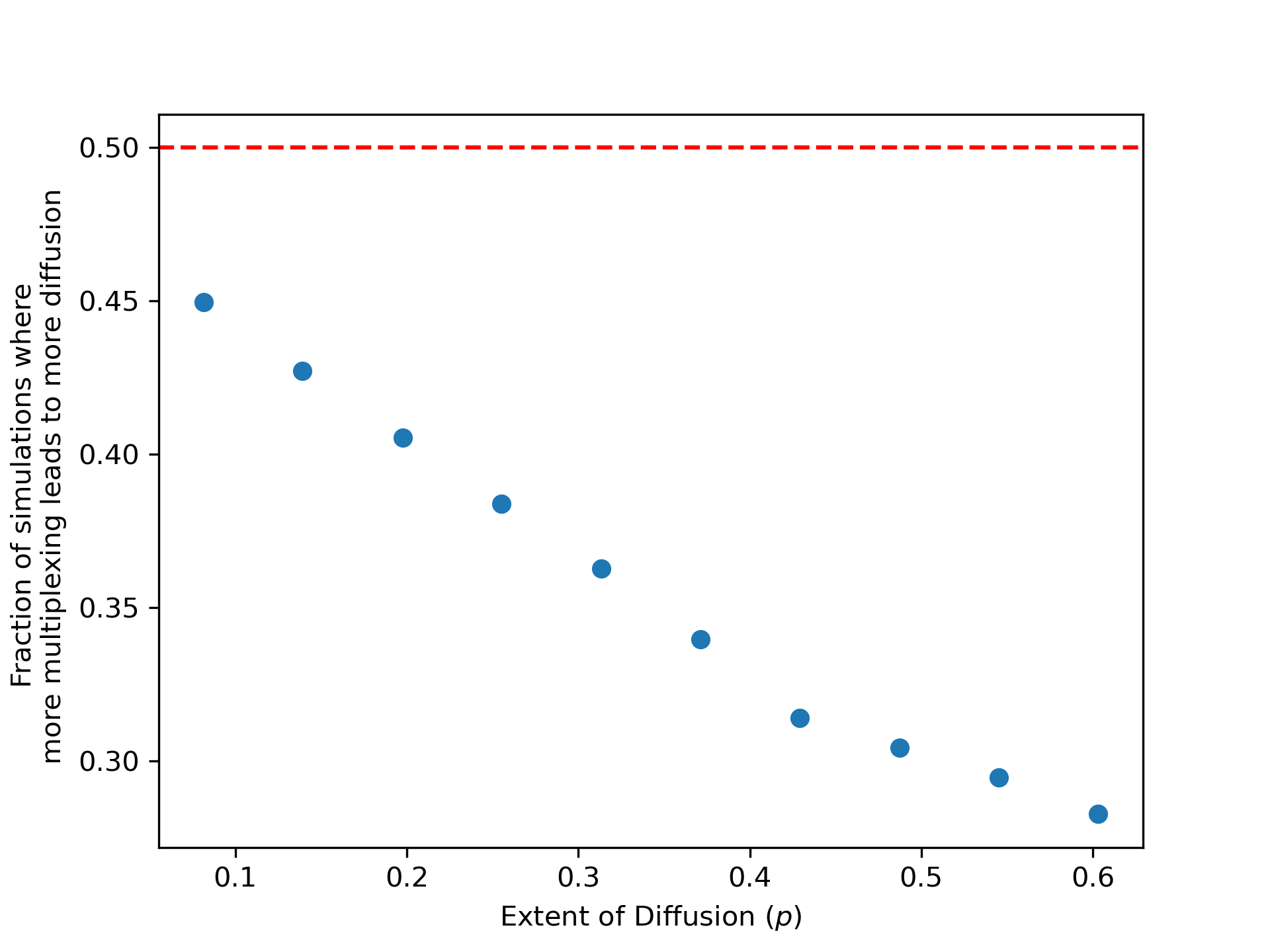
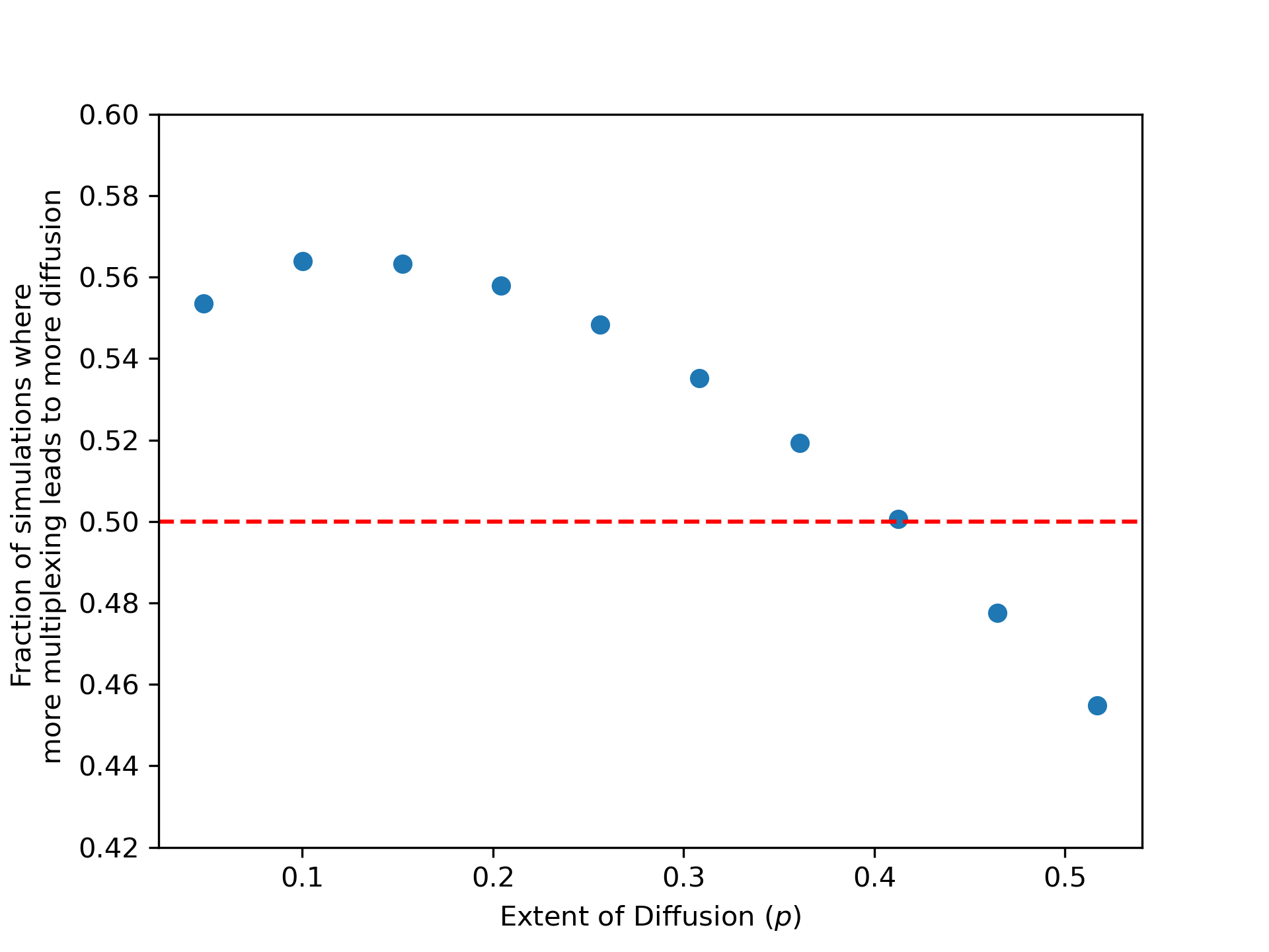
In Figure 6 we plot the fraction of simulation runs where more multiplexing leads to more diffusion against the extent of diffusion in the network . In panel A, we plot the results for simple diffusion. We find that higher multiplexing is consistently associated with lower diffusion levels, as in our theoretical results.
In panel B we see the nonmonotonicity from the countervailing forces in complex diffusion that we mentioned in Section 3.3. We also see a confirmation of the theoretical results. At low levels of diffusion, the steady state diffusion is increasing in multiplexing, and for high diffusion levels, the steady state diffusion is decreasing in multiplexing.
4. Concluding Discussion
Our study began by examining patterns of multiplexing in two large data sets. We next showed that multiplexing systematically impacts diffusion, via both experimental evidence and theoretical modeling.
Our findings highlight the need for future work on incentives to multiplex and the consequences of multiplexing decisions. There are several immediate directions to explore. For example, our results suggest that the deeper the need to form reinforced or supported (i.e., multiplexed) relationships, the greater the potential inefficiencies in certain domains. In particular, those who are under weaker institutions or have limited resources may face a greater need to multiplex relative to their richer counterparts. Consequently, they may experience both reduced access to information and increased susceptibility to the spread of social norms that are described by complex contagion dynamics—a susceptibility that may be beneficial or detrimental.
There is also a need for further development of measures and methods of analyzing multiplexed networks. We defined one of many potential measures of how multiplexed a network is, as well as one of many potential partial orders. Understanding which measures are most appropriate in which settings is a subject for further research.
To close, we report two other patterns that we found in the data. For both of the following calculations, we use the multiplexing score that we defined in Section 2.4:
where represents either an individual or a household, depending on the analysis.
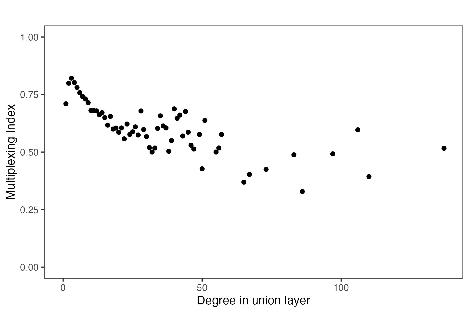
The first pattern is that higher-degree households are less multiplexed. We restrict our attention to the elicited layers in the RCT villages: the social, kerorice, advice, and decision layers. Figure 7 depicts a binned scatter plot where we can see that households that have higher degree (aggregated across layers) have lower levels of multiplexing.
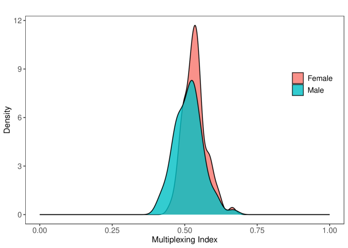
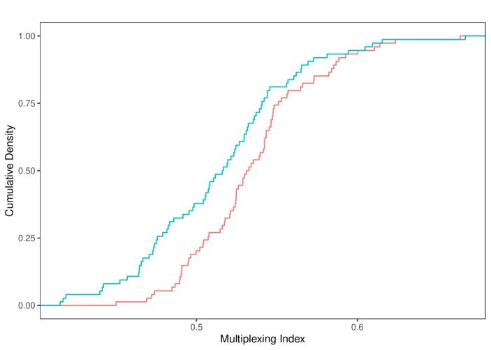
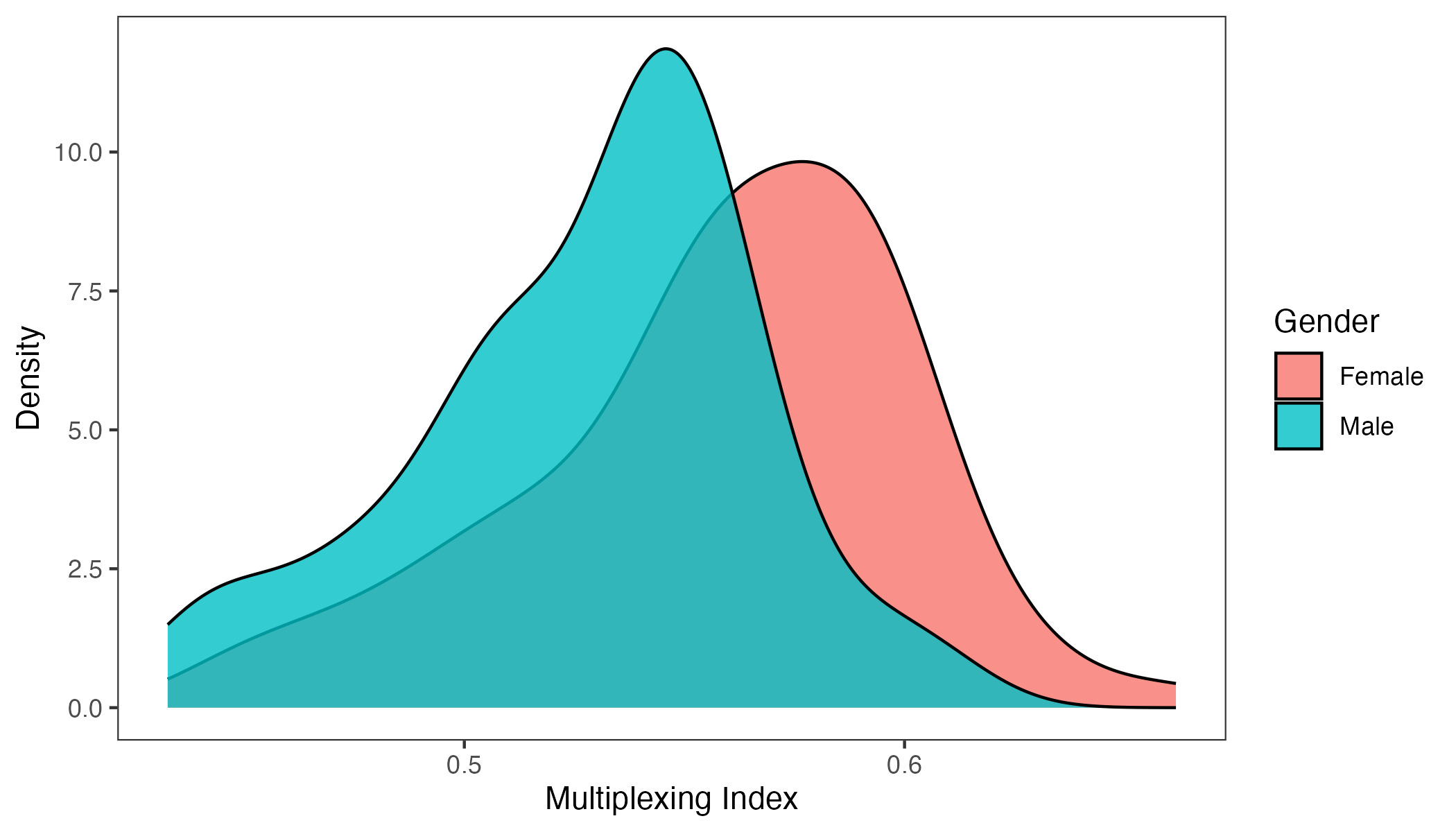
The second pattern is that women’s networks are significantly more multiplexed than those of men. Here we use the microfinance villages, where we have access to individual-level network data. We focus on the social, kerorice, advice, decision, money, temple, and medic layers. For each village , we aggregate this score at the gender level: , where . Figure 8 shows the density curves for these multiplexing scores across the villages, as well as for each individual treated as a separate observation. The distributions reveal that women’s networks are systematically more multiplexed. In Supplemental Appendix Figure S3 we include the same analysis with a different wave of data, and see an even starker difference.
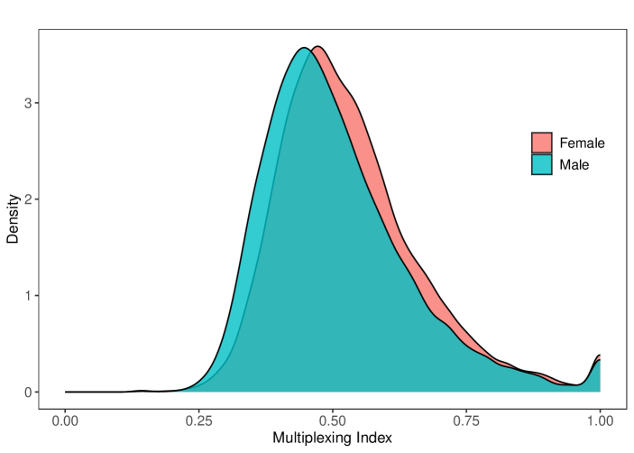
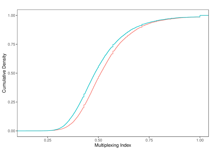
This result could help explain results of Beaman and Dillon (2018), who found unexplained differences in diffusion by gender. To understand potential sources of gender differences in multiplexing, note that women in rural Indian communities often marry across village boundaries (though frequently still within the constraints of caste/jati endogamy) and most of these marriages are virilocal—requiring the wife to move into the husband’s house (Rosenzweig and Stark, 1989; Rao and Finnoff, 2015). As a consequence, women often rely on affinal kin and over time need to “rebuild” their networks (Hruschka et al., 2023). This occurs in conjunction with the expectation that these women take on various responsibilities, including agricultural work, managing the household, preparing meals, and raising children. Such constraints on available relationships while serving multiple roles can plausibly result in high levels of multiplexing, an interesting subject for further research.
References
- Ambrus et al. (2014) Ambrus, A., M. Mobius, and A. Szeidl (2014): “Consumption risk-sharing in social networks,” American Economic Review, 104, 149–182.
- Atkisson et al. (2019) Atkisson, C., P. J. Górski, M. O. Jackson, J. A. Hołyst, and R. M. D’Souza (2019): “Why understanding multiplex social network structuring processes will help us better understand the evolution of human behavior,” forthcoming: Evolutionary Anthropology.
- Banerjee et al. (2024a) Banerjee, A., A. G. Chandrasekhar, S. Dalpath, E. Duflo, J. Floretta, M. O. Jackson, H. Kannan, F. N. Loza, A. Sankar, A. Schrimpf, et al. (2024a): “Selecting the Most Effective Nudge: Evidence from a Large-Scale Experiment on Immunization,” Econometrica, forthcoming.
- Banerjee et al. (2019) Banerjee, A., A. G. Chandrasekhar, E. Duflo, and M. O. Jackson (2019): “Using gossips to spread information: Theory and evidence from two randomized controlled trials,” The Review of Economic Studies, 86, 2453–2490.
- Banerjee et al. (2024b) Banerjee, A. V., E. Breza, A. G. Chandrasekhar, E. Duflo, M. O. Jackson, and C. Kinnan (2024b): “Changes in Social Network Structure in Response to Exposure to Formal Credit Markets,” Review of Economic Studies, 91:3, 1331–72.
- Banerjee et al. (2013) Banerjee, A. V., A. G. Chandrasekhar, E. Duflo, and M. O. Jackson (2013): “Diffusion of Microfinance,” Science, 341, DOI: 10.1126/science.1236498, July 26 2013.
- Beaman and Dillon (2018) Beaman, L. and A. Dillon (2018): “Diffusion of agricultural information within social networks: Evidence on gender inequalities from Mali,” Journal of Development Economics, 133, 147–161.
- Becker et al. (2020) Becker, S. O., Y. Hsiao, S. Pfaff, and J. Rubin (2020): “Multiplex network ties and the spatial diffusion of radical innovations: Martin Luther’s leadership in the early reformation,” American Sociological Review, 85, 857–894.
- Bianconi (2018) Bianconi, G. (2018): Multilayer networks: structure and function, Oxford university press.
- Billand et al. (2023) Billand, P., C. Bravard, S. Joshi, A. S. Mahmud, and S. Sarangi (2023): “A model of the formation of multilayer networks,” Journal of Economic Theory, 213, 105718.
- Boccaletti et al. (2014) Boccaletti, S., G. Bianconi, R. Criado, C. I. Del Genio, J. Gómez-Gardenes, M. Romance, I. Sendina-Nadal, Z. Wang, and M. Zanin (2014): “The structure and dynamics of multilayer networks,” Physics reports, 544, 1–122.
- Centola (2010) Centola, D. (2010): “The Spread of Behavior in an Online Social Network Experiment,” Science, 329: 5996, 1194–1197, DOI: 10.1126/science.1185231.
- Cheng et al. (2021) Cheng, C., W. Huang, and Y. Xing (2021): “A theory of multiplexity: Sustaining cooperation with multiple relations,” Available at SSRN 3811181.
- Contractor et al. (2011) Contractor, N., P. Monge, and P. M. Leonardi (2011): “Network Theory— multidimensional networks and the dynamics of sociomateriality: bringing technology inside the network,” International Journal of Communication, 5, 39.
- Dickison et al. (2016) Dickison, M. E., M. Magnani, and L. Rossi (2016): Multilayer social networks, Cambridge University Press.
- Dodds and Watts (2004) Dodds, P. S. and D. J. Watts (2004): “Universal behavior in a generalized model of contagion,” Physical review letters, 92, 218701.
- Elliott et al. (2022) Elliott, M., B. Golub, and M. V. Leduc (2022): “Supply network formation and fragility,” American Economic Review, 112, 2701–2747.
- Fafchamps and Gubert (2007) Fafchamps, M. and F. Gubert (2007): “Risk sharing and network formation,” American Economic Review, 97, 75–79.
- Granovetter (1978) Granovetter, M. S. (1978): “Threshold models of collective behavior,” American journal of sociology, 83, 1420–1443.
- Hruschka et al. (2023) Hruschka, D. J., S. Munira, and K. Jesmin (2023): “Starting from scratch in a patrilocal society: how women build networks after marriage in rural Bangladesh,” Philosophical Transactions of the Royal Society B, 378, 20210432.
- Hu et al. (2013) Hu, Y., D. Zhou, R. Zhang, Z. Han, C. Rozenblat, and S. Havlin (2013): “Percolation of interdependent networks with intersimilarity,” Physical Review E—Statistical, Nonlinear, and Soft Matter Physics, 88, 052805.
- Jackson (2008) Jackson, M. O. (2008): Social and economic networks, Princeton: Princeton University Press.
- Jackson et al. (2024) Jackson, M. O., S. M. Nei, E. Snowberg, and L. Yariv (2024): “The Dynamics of Networks and Homophily,” SSRN Working Paper https://papers.ssrn.com/abstract=4256435, .
- Jackson and Zenou (2014) Jackson, M. O. and Y. Zenou (2014): “Games on Networks,” Handbook of Game Theory, Elsevier, edited by Young, H.P. and Zamir, S.
- Javanmard and Montanari (2013) Javanmard, A. and A. Montanari (2013): “Model selection for high-dimensional regression under the generalized irrepresentability condition,” in Proceedings of the 26th International Conference on Neural Information Processing Systems-Volume 2, 3012–3020.
- Jia et al. (2015) Jia, J., K. Rohe, et al. (2015): “Preconditioning the lasso for sign consistency,” Electronic Journal of Statistics, 9, 1150–1172.
- Kivela et al. (2014) Kivela, M., A. Arenas, J. P. Gleeson, Y. Moreno, and M. A. Porter (2014): “Multilayer Networks,” arXiv:1309.7233v4 [physics.soc-ph].
- Kobayashi and Onaga (2023) Kobayashi, T. and T. Onaga (2023): “Dynamics of diffusion on monoplex and multiplex networks: A message-passing approach,” Economic Theory, 76, 251–287.
- Larson and Rodriguez (2023) Larson, J. M. and P. L. Rodriguez (2023): “The risk of aggregating networks when diffusion is tie-specific,” Applied Network Science, 8, 21.
- Lee et al. (2016) Lee, J. D., D. L. Sun, Y. Sun, and J. E. Taylor (2016): “Exact post-selection inference, with application to the lasso,” The Annals of Statistics, 44, 907–927.
- Luo and Li (2016) Luo, W. and B. Li (2016): “Combining eigenvalues and variation of eigenvectors for order determination,” Biometrika, 875–887.
- Morelli et al. (2017) Morelli, S. A., D. C. Ong, R. Makati, M. O. Jackson, and J. Zaki (2017): “Empathy and well-being correlate with centrality in different social networks,” Proceedings of the National Academy of Sciences, 114, 9843–9847.
- Morris (2000) Morris, S. (2000): “Contagion,” Review of Economic Studies, 67 (1), 57–78.
- Munshi and Rosenzweig (2009) Munshi, K. and M. Rosenzweig (2009): “Why is Mobility in India so Low? Social Insurance, Inequality, and Growth,” mimeo.
- Pastor-Satorras and Vespignani (2000) Pastor-Satorras, R. and A. Vespignani (2000): “Epidemic Spreading in Scale-Free Networks,” Physical Review Letters, 86 (14), 3200–3203.
- Rao and Finnoff (2015) Rao, S. and K. Finnoff (2015): “Marriage migration and inequality in India, 1983–2008,” Population and Development Review, 41, 485–505.
- Rohe (2015) Rohe, K. (2015): “Preconditioning for classical relationships: a note relating ridge regression and OLS p-values to preconditioned sparse penalized regression,” Stat, 4, 157–166.
- Rosenzweig and Stark (1989) Rosenzweig, M. R. and O. Stark (1989): “Consumption smoothing, migration, and marriage: Evidence from rural India,” Journal of political Economy, 97, 905–926.
- Sacerdote (2001) Sacerdote, B. (2001): “Peer effects with random assignment: Results for Dartmouth roommates,” The Quarterly journal of economics, 116, 681–704.
- San Román (2024) San Román, D. (2024): “Multiplexed Network Formation and Bonacich Centrality,” Available at SSRN 4704738.
- Simmel (1908) Simmel, G. (1908): Sociology: Investigations on the Forms of Sociation, Leipzig: Duncker and Humblot.
- Taylor and Tibshirani (2015) Taylor, J. and R. J. Tibshirani (2015): “Statistical learning and selective inference,” Proceedings of the National Academy of Sciences, 112, 7629–7634.
- Townsend (1994) Townsend, R. M. (1994): “Risk and Insurance in Village India,” Econometrica, 62, 539–591.
- Walsh (2019) Walsh, A. M. (2019): “Games on multi-layer networks,” .
- Wasserman and Faust (1994) Wasserman, S. and K. Faust (1994): Social Network Analysis, Cambridge: Cambridge University Press.
- Yağan and Gligor (2012) Yağan, O. and V. Gligor (2012): “Analysis of complex contagions in random multiplex networks,” Physical Review E—Statistical, Nonlinear, and Soft Matter Physics, 86, 036103.
- Zenou and Zhou (2024) Zenou, Y. and J. Zhou (2024): “Games on Multiplex Networks,” Available at SSRN 4772575.
- Zhao and Yu (2006) Zhao, P. and B. Yu (2006): “On model selection consistency of Lasso,” The Journal of Machine Learning Research, 7, 2541–2563.
- Zhu et al. (2019) Zhu, S.-S., X.-Z. Zhu, J.-Q. Wang, Z.-P. Zhang, and W. Wang (2019): “Social contagions on multiplex networks with heterogeneous population,” Physica A: Statistical Mechanics and its Applications, 516, 105–113.
Appendix A Proofs
Proof of Proposition 1: We adopt the notation from Proposition 2, as given independent probabilities of infection of neighbors, the probability that an individual with connection profile on network becomes infected is then (from (3.3) given by
If the change is to network in which this individual is less multiplexed then their connection profile is for some integer , and then their probability of being infected is
The second probability is larger than the first if and only if
which simplifies to
This holds if and only if
which is the claimed condition.
Proof of Proposition 2: Following the argument from the proof of Proposition 1, for any equation 3.4 has a higher solution for the less multiplexed type. Thus, starting with the steady state for the more multiplexed distribution, the new rates for all individuals are weakly and sometimes strictly higher for the less multiplexed distribution. This leads to a higher . Iterating, this converges upward for all types to a limit which is the steady state. Conversely, if condition 3.1 is reversed, the convergence is downward for all types.
Proof of Proposition 3: It is enough to consider an individual with one change in their links where a multiplexed link to is then split to two neighbors , each of which is connected to on a different layer and where was initially not connected to . Our focus is on the pivotal cases:
-
(1)
The number of infected messages has already received from other neighbors is either or . (That both of these cases can occur with positive probability uses the condition that , so that there are at least layer-connections from to others besides .)
-
(2)
At least one of the neighbors and is infected.
The conditional probability (given that one is in one of these four cases) that gets infected can be found in the table below. The top entry in each cell represents the multiplexing scenario and the bottom represents the unmultiplexed case.
| both infected | ||
|---|---|---|
| one of infected |
The inequality indicates which probability is larger. The column (aggregating over both rows which have positive probability) has strictly higher probability for the unmultiplexed case, while the column has strictly higher probability for the multiplexed case. Let be the probability on the first column and on the second column, and note that the conditional probability of the first row is and the second row is . The differences in overall probabilities of infection of the multiplexed minus unmultiplexed is then
Given that , then this expression has the sign of . The proof is then completed by noting that for high enough the first column becomes more likely than the second, and for low enough the second column becomes more likely than the first.This is where the condition that is invoked. With independent signal transmission across layers, for low enough , it is strictly more probable to have fewer than more signals from the connections other than , and thus . These probabilities are continuous in and so this holds for some . The reverse is true for high enough .
Proof of Proposition 4: We begin with the case of sufficiently low and high . In that case will also be low (an absolute bound is simply as that is a crude upper bound on the infection rate of any given node that always has all neighbors infected and needs only one signal). Then we can invoke Proposition 3 for each connection configuration (noting that there are a finite number of them, taking the min over the ), and then the remaining argument is analogous to the proof of Proposition 2. The reverse holds for the case of sufficiently high and low .
Proposition 5.
The relation is acyclic.
Proof of Proposition 5 Recall that we denote the set of layers a link belongs to by . Define the total multiplexity index of a multigraph as .
We show that if , then . By our definition of , we know that there exist nodes and layers such that and , all else being equal. We only focus on the contribution of these edges in total multiplexing index since all other links are identical across the two multigraphs. For the multigraph , this can be represented as , while for the less multiplexed graph , the contribution of these edges can be written as . We can then write the difference in total multiplexing between and as
By , we know that (recall that we assumed and were linked in at least two layers), hence
Now, assume that there exists a cycle such that we have a sequence of multigraphs with . But our proof implies , which gives us a contradiction. Hence the relation is acyclic.
Supplementary Appendix:
Multiplexing in Networks and Diffusion
by Chandrasekhar, Chaudhary, Golub, Jackson
A.1. Supplementary Figures
Figure S1 plots the results from Table 2. and both the 90% and 95% confidence intervals for each of the distinct layers are plotted. Seed centrality in the jati network is not statistically significantly associated with diffusion (). Seed centrality in the advice, social, and kerorice networks all are significantly positively associated with diffusion. The point estimates are large, roughly a 59% increase.
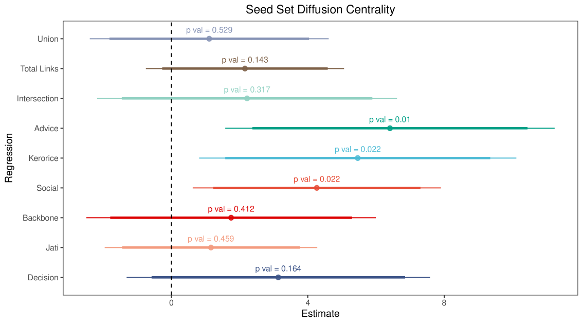
Here we redo the analysis from Figure 8, but instead using the individual network data from Microfinance villages collected as part of Wave I of data collection in Banerjee et al. (2013) (instead of Wave II).202020We have individual-level gender-distinguished data in the Wave I network survey, which elicited links from % of the households, giving us information on % of the links.
A.2. Supplementary Tables
In Table S1, we redo Table 2 but with the aggregate networks of union, intersection, and backbone constructed without including jati (the total link network is directed and never included jati).
| No. Calls Received | |||||||||
| 1 | 2 | 3 | 4 | 5 | 6 | 7 | 8 | 9 | |
| Social | |||||||||
| () | |||||||||
| [] | |||||||||
| Kero/Rice | |||||||||
| () | |||||||||
| [] | |||||||||
| Advice | |||||||||
| () | |||||||||
| [] | |||||||||
| Decision | |||||||||
| () | |||||||||
| [] | |||||||||
| Jati | |||||||||
| () | |||||||||
| [] | |||||||||
| Union | |||||||||
| () | |||||||||
| [] | |||||||||
| Intersection | |||||||||
| () | |||||||||
| [] | |||||||||
| Backbone | |||||||||
| () | |||||||||
| [] | |||||||||
| Total Links | |||||||||
| () | |||||||||
| [] | |||||||||
| Num.Obs. | |||||||||
| R2 | |||||||||
| Dep Var mean | |||||||||
-
•
Note: Robust standard errors are given in parentheses and p-values in square brackets. Controls added: number of households, its powers, and a dummy for number of seeds in the village. Exogenous variables are the sum of Diffusion Centrality for seeds in each village for the layer. Exogenous variables have been standardized. None of the aggregate layers (union, intersection, backbone and total links) uses jati as an input.
| Network | PC1 | PC2 | PC3 | PC4 | PC5 | PC6 | PC7 | PC8 | PC9 |
|---|---|---|---|---|---|---|---|---|---|
| social | 0.37 | -0.04 | -0.03 | 0.18 | -0.55 | 0.69 | -0.13 | -0.17 | -0.07 |
| kerorice | 0.38 | 0.02 | 0.01 | 0.07 | -0.43 | -0.69 | -0.38 | -0.17 | -0.11 |
| money | 0.41 | 0.06 | 0.02 | 0.11 | 0.07 | 0.01 | -0.14 | 0.72 | 0.52 |
| advice | 0.40 | 0.08 | 0.03 | 0.07 | 0.51 | 0.11 | -0.22 | 0.16 | -0.70 |
| decision | 0.40 | 0.07 | 0.02 | 0.12 | 0.47 | 0.03 | -0.01 | -0.62 | 0.45 |
| medic | 0.39 | 0.05 | 0.01 | 0.07 | -0.12 | -0.17 | 0.88 | 0.04 | -0.14 |
| temple | 0.24 | 0.06 | 0.02 | -0.96 | -0.05 | 0.08 | -0.02 | -0.03 | 0.03 |
| jati | 0.10 | -0.66 | -0.74 | -0.04 | 0.08 | -0.04 | 0.01 | 0.02 | 0.00 |
| distance | -0.07 | 0.73 | -0.68 | 0.02 | -0.05 | 0.01 | -0.02 | -0.01 | 0.00 |
| Network | PC1 | PC2 | PC3 | PC4 | PC5 |
|---|---|---|---|---|---|
| social | 0.49 | 0.03 | -0.58 | 0.52 | -0.39 |
| kerorice | 0.50 | 0.04 | -0.39 | -0.48 | 0.60 |
| advice | 0.50 | 0.05 | 0.37 | -0.51 | -0.59 |
| decision | 0.49 | 0.05 | 0.61 | 0.50 | 0.37 |
| jati | 0.09 | -1.00 | 0.02 | 0.00 | 0.00 |
| layer | df | R.sq. | F-stat | p-val | F-stat marginal | p-val marginal |
|---|---|---|---|---|---|---|
| Advice | 1 | 0.233 | 20.057 | 0.000 | ||
| Jati | 2 | 0.263 | 2.628 | 0.110 | 2.628 | 0.110 |
| Decision | 3 | 0.272 | 1.728 | 0.186 | 0.834 | 0.365 |
| Kero/Rice | 4 | 0.293 | 1.768 | 0.162 | 1.804 | 0.184 |
| Social | 5 | 0.293 | 1.306 | 0.278 | 0.006 | 0.938 |
A.3. Algorithms
-
•
: Set of all nodes in the network,
-
•
: Set of susceptible nodes at time
-
•
: Set of infected nodes at time
-
•
: State of node at time , where
-
•
: Number of exposures (infections) node is exposed to at time