Multiplicity of electron- and photon-seeded electromagnetic showers
at multi-petawatt laser facilities
Abstract
Electromagnetic showers developing from the collision of an ultra-intense laser pulse with a beam of high-energy electrons or photons are investigated under conditions relevant to future experiments on multi-petawatt laser facilities. A semi-analytical model is derived that predicts the shower multiplicity, i.e. the number of pairs produced per incident seed particle (electron or gamma photon). The model is benchmarked against particle-in-cell simulations and shown to be accurate over a wide range of seed particle energies (100 MeV - 40 GeV), laser relativistic field strengths (), and quantum parameter (ranging from 1 to 40). It is shown that, for experiments expected in the next decade, only the first generations of pairs contribute to the shower while multiplicities larger than unity are predicted. Guidelines for forthcoming experiments are discussed considering laser facilities such as Apollon and ELI Beamlines. The difference between electron- and photon seeding and the influence of the laser pulse duration are investigated.
I Introduction
Since its first developments 90 years ago [1, 2, 3], quantum electrodynamics (QED) has been established as the best tested, most precise physical theory. Its subbranch, strong-field QED (SF-QED), which describes light-matter interaction in the presence of very strong electromagnetic fields, however, remains only partially tested. Over the last decade, it has become the focus of extensive research [4, 5] as new laser and accelerator facilities worldwide allow us to put this theory to the test.
Among the most exotic phenomena predicted by SF-QED is the (potentially copious) production of electron-positron pairs in so-called QED cascades developing in strong electromagnetic fields. At the heart of these cascades are two QED processes: nonlinear Breit-Wheeler pair production [6], that is the decay of a photon into an electron-positron pair under the influence of a strong electromagnetic field, and nonlinear Compton scattering that is in the emission of a high-energy photon by an electron (or positron) subjected to a strong electromagnetic field [7, 8, 9].
These exotic processes are omnipresent in extreme astrophysical environments, such as neutron stars, pulsars, and magnetars [10, 11, 12], where intense magnetic fields give rise to the copious emission of electron-positron pairs and high-energy photons [13, 14]. Creating pair plasmas in the laboratory would be crucial to understanding the dynamics of highly magnetized environments and testing SF-QED. While it still poses a significant challenge [15], the advent of laser systems of unprecedented power may soon allow for the creation of QED cascades in the laboratory and the abundant generation of pairs in the laboratory.
Indeed, several multi-petawatt laser facilities are being developed worldwide [16, 17]: Apollon [18], CoReLS [19], ELI [20], EP-OPAL [21], Vulcan [22] or ZEUS [23]. These facilities will allow to deliver ultra-short (20 fs - 150 fs) light pulses with intensities beyond W/cm2 [24]. Various approaches have been proposed to use such light pulses to drive abundant pair production. These include irradiating a solid target with an ultra-intense light pulse [25, 26, 27, 28, 29], colliding two (to several) laser pulses to construct electromagnetic fields structures (e.g. rotating field) maximizing pair production [30, 31, 32, 33, 34, 35, 36, 37, 38], colliding a laser pulse with a beam of relativistic electrons or photons [39, 40, 41, 42, 43, 44], among others [45, 46].
Creating a dense plasma of pairs in the laboratory would most certainly require generating a particular type of QED cascade,
called an avalanche, in which the number of pairs increases exponentially with time [47, 48, mercuri-baron_2024]. Entering the avalanche regime however often requires the use of several ultra-intense laser beams synchronized in space and time to build up electromagnetic field configurations allowing for particle re-acceleration and thus sustaining the avalanche process.
This renders the experiment currently inaccessible.
An alternative, albeit less efficient, method involves colliding a beam of ultrarelativistic electrons
[42, 41] or photons [43] against the intense laser pulse, leading to so-called electromagnetic showers.
In this scenario, re-acceleration in the laser field has limited influence and the resulting shower (electron, positron, and photons) draws its energy from the initial (seed) electron or photon beam[49, 50].
To this day only the seminal SLAC E-144 experiment [39] has demonstrated electron-positron production from the collision of an ultra-relativistic electron beam with a high-intensity laser pulse.
However, due to the quite limited intensity of the laser employed in this experiment, very few pairs were produced: pairs/21962 collisions.
Exploiting the capacities of multi-beam, multi-petawatt laser facilities will allow to enter the regime of abundant pair production, where any seed particle (electron or photon) injected into the focal volume of the ultra-intense laser pulse will lead to at least an electron-positron pair.
This was for instance demonstrated through three-dimensional particle-in-cell simulations exploring conditions relevant to the Apollon laser facility for which it was shown that electron-seeded showers could lead to the production of high-density sources of ultra-relativistic electron-positron pairs accompanied by a brilliant flash of high-energy photons.
In this paper, we explore both electron- and photon-seeded showers to predict a crucial observable in future experiments: the number of produced pairs.
More precisely, we derive a semi-analytical model that predicts the number of pairs produced per incident (seed) particle,
henceforth referred to as the shower multiplicity. This model builds on previous works by Blackburn et al. [42] for electron-seeded showers and Mercuri-Baron et al. [43]
for photon-seeded ones. By alleviating some hypotheses made in these previous works, we significantly extend their domain validity to cover the region of parameters (seed-particle energy, laser field strength, pulse duration, etc) relevant to future experiments at multi-petawatt laser facilities111While the model can be generalized to any laser beam polarization and angle of incidence, the results are specifically presented for linear polarization and head-on collision.. Throughout this paper, the model is tested against particle-in-cell (PIC) simulations performed with the open-source code Smilei [51] accounting for the relevant QED processes [52, 53, 54, 55, 56]. Doing so allows us to test the hypotheses of the model (see Sec. II.1 for details) as well as to get a deeper insight into the physics of electromagnetic showers.
The paper is structured as follows. In Sec. II we describe a reduced model that predicts the number of pairs in a one-dimensional geometry. A key hypothesis introduced here is to assume that, under conditions relevant to our study, only the first generations of pairs contribute to the shower. The model is benchmarked against PIC simulations in Sec. III. This allows us to discuss the domain of validity of the model as well as to extract physical insight into the shower development and provide guidelines for future experiments. We discuss in detail the difference between photon and electron seeding, and that between short (few cycles) and long (150 fs) laser pulses. In Sec. IV, we extend our predictions to a realistic three-dimensional case and test our extended model against PIC simulations. A full theoretical guide map for the shower multiplicity is derived and discussed as a function of the incident (seed) particle energy and laser field strength (intensity) focusing in particular on the cases of Apollon-like (Ti:Sapphire, 20 fs-long) and ELI-Beamlines-A4-Aton-like (Ne:Glass, 150 fs-long) laser pulses. Finally, we summarize our conclusions in Sec. V.
II Reduced model
SI units and standard notations for physical constants will be used throughout the paper: stands for the speed of light in vacuum, for the electron mass, for the elementary charge, for the fine structure constant, for the permittivity of vacuum and for the Compton time.
II.1 Objectives and hypotheses of the model
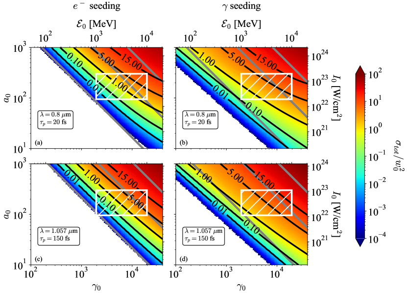
We present a reduced model for electromagnetic showers developing in the head-on collision of a high-energy electron or photon beam with an ultra-intense laser pulse, see Fig. 1 (a) and (b).
The initial (seed) beam is considered to be a point-like (zero spatial extension and angular aperture) beam of initially monoenergetic particles
with energy for photons and for charged particles. In this work, we will focus on ultra-high energy seed particles, , focusing
in particular on the range , i.e. energies in the range 50 MeV - 20 GeV.
Furthermore, we will consider optical laser systems with a micrometric wavelength , and large
relativistic field strength parameter (with the maximum laser electric field and
the laser angular frequency).
As our interest lies in future experiments on multi-petawatt laser systems,
we focus on ,
corresponding to (with the peak laser intensity).
Furthermore, predictions of the number of produced pairs will be discussed for two types of laser systems:
ultra-short (20 fs) Ti:Sapphire () laser pulses as delivered at Apollon, CoReLS, or ZEUS,
and longer (150 fs) Nd:Glass () laser pulses as delivered by the L4 ATON laser beam at ELI Beamlines.
The range of parameters discussed in this work is reported in Fig. 1(c) considering and a full-width-at-half-maximum-intensity laser pulse duration . Superimposed is a rectangular region that corresponds to seed particle energies in between 1 and 10 GeV and field strengths in between and computed considering a 1PW or 10 PW Gaussian laser pulse focused with an angular aperture . It is relevant to most forthcoming experiments on multi-petawatt laser systems.
We also report the value of the maximum quantum parameter a particle (either photon, electron or positron) with energy can achieve colliding head-on with an electromagnetic wave of relativistic field strength :
| (1) |
In this representation, contours of iso- are oblique lines and iso-contours and are reported as grey lines.
We further report two regions of interest.
The first, blue one, corresponds to the region of validity of the model developed by Blackburn et al. [42]
for electron-seeded showers. It is limited to low values which is not of direct interest for
multi-petawatt laser facilities, but rather corresponds to regimes explored coupling standard accelerators with near-100 TW laser systems,
as planned for experiments such as LUXE or FACET-II.
The second, in red, corresponds to the domain of validity of the model proposed by Mercuri-Baron et al. [43]
for photon-seeded showers. More precisely, it corresponds to the limit of the so-called soft-shower regime in which pair production
is dominated by the decay of the seed photons only. This region covers part, but not all of the (green-hatched) region of interest
for multi-petawatt laser systems.
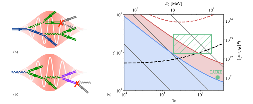
Our objective is to extend the region of validity of both models to cover the whole region of interest for multi-petawatt laser systems.
To do so, we will go beyond some of the hypotheses made in the previous models.
To extend Blackburn’s model to higher , we (i) make the distinction between rates and probabilities,
and (ii) include the contribution of intermediate-energy electrons to the shower.
To extend Mercuri-Baron’s model [43], we go beyond the soft-shower regime and account for the secondary pairs considering that primary pairs can radiate away
high-energy photons that can, in turn, decay into new electron-positron pairs [see Fig. 1(b)].
By doing so, we derive a set of equations that can be integrated numerically. To make this model tractable and gain insights into the development of the shower, we retain some hypotheses which we now detail.
First, we split all species (photons, electrons, and positrons) into successive generations which we treat separately, each species generation being described by its own distribution function (for a treatment of the full distribution functions see Appendix A). When considering electron-seeded showers [see Fig. 1(a)], the seed electrons will emit a first generation of (primary) high-energy photons that may then decay in a first generation of (primary) electron-positron pairs. Our model of electron-seeded showers considers that these primary pairs account for most of the produced pairs and we neglect secondary photons that can be emitted by those primary pairs. Note that the number of pairs is not, here, limited to the number of seed electrons as those electrons may emit more than a single photon. This is different from the case of photon-seeded showers [see Fig. 1(b)] for which going beyond the soft-shower limit is needed if one wants to enter regimes where the number of produced pairs exceeds that of seed photons. In the photon-seeded model, one thus allows the primary pairs222As further discussed in Sec. II.3, we actually consider that only one particle (electron or positron) per primary pair can further contribute to the cascade. to radiate high-energy photons that can decay into a second generation of pairs. Further emission of high-energy photons by this second generation of pairs will however be neglected. We will show in Sec. III.2 that considering only the first two generations provides an excellent approximation in many regimes of interest, and we will give an intuitive justification of why this is so.
Second, we assume that all particles participating in high-energy photon emission and pair production are ultra-relativistic () at all times. This allows us to approximate electron and positron velocity as that of light and to consider that high-energy photons and electron-positron pairs are emitted/created with a momentum aligned with that of the particle they originate from. We further assume that all particles propagate in the same direction, , and will in particular neglect the change of momentum of the charged particles in the laser electromagnetic field. This is a good approximation assuming (satisfied for parameters of interest for this study). As a consequence, all particles experience at any given time the same electric and magnetic fields and , with denoting the particles’ position at time . While the model developed in Secs. II.2 and II.3 can be applied to arbitrary polarizations, within this work, we will focus on linearly-polarized electromagnetic pulses with an electric field:
| (2) |
and magnetic field .
Here, we have considered a sin2 intensity profile with its full-width-at-half-maximum-intensity. It follows that knowing a particle’s energy at any time uniquely defines its time-dependent quantum parameter333Valid for photons as well as electrons or positrons.
| (3) |
Third, the rate of photon emission by electrons and positrons is computed using the average charged particle energy and the corresponding quantum parameter. This approximation, which we have found to provide a good prediction for the spectrum of emitted photons, is different from the one considered by Blackburn in his model of electron-seeded showers. Indeed, in Ref. [42], the authors compute the rate of photon emission using the initial (seed) electron energy (even though they do account for energy loss when computing the electron quantum parameter). This approach can be justified in the low regime where pair production is dominated by those photons that have been emitted by the highest energy electrons. It does not hold however in the regime of interest for his work and radiation losses have to be accounted for.
Last, as we are mostly interested in the range of parameters that will be explored by multi-petawatt laser facilities (), the processes of high-energy photon emission (nonlinear inverse Compton scattering) and electron-positron pair production (Breit-Wheeler process) are described by their (energy) differential rates computed in the locally constant cross-field approximation (LCFA):
| (4) | |||||
| (5) |
where denotes the probability for an electron (equivalently positron) of energy and quantum parameter to emit a high-energy photon with energy in between and between times and , while denotes that of a photon to decay into a pair with the electron carrying an energy in between and . The functions and are reported in Appendix B. Integrating these differential rates over all possible daughter particle energy [photons for Eq. (4) and electrons/positrons for Eq. (5)] leads to the photon emission and pair production rates
| (6) | |||
| (7) |
where the functions and and their asymptotic limits are reported in Appendix B.
In Fig.1(c), black and red dotted lines report the values of (,) for which and , respectively. The values of (,) for which
(with ) are also reported as a blue solid line defining the regime of validity of the model proposed by Blackburn et al. [42].
It is clear that, in the regime of interest for future experiments
at multi-petawatt laser facilities, abundant high-energy photon emission
is expected on timescales of the order of or shorter than the optical cycle (). In contrast, the characteristic time for
a photon to decay into an electron-positron pair will be larger than the
optical cycle, yet shorter than the characteristic pulse duration (considering ).
In what follows, we describe the models that have been developed for electron-seeded and photon-seeded cascades. In both cases, we first give the governing equations for the distribution functions of the successive generation of species (electrons, positrons and photons) participating in the shower. We then derive our model and discuss our assumptions. Last we briefly summarise how the model is used to compute the final number of pairs produced per incident (seed) particle, henceforth referred to as the shower multiplicity.
II.2 Electron seeding
When the shower is seeded by an incident electron beam, we need to follow the dynamics of the seeding electrons through their distribution function , the first generation of gamma photons, i.e. those emitted by the seeding electron, though their distribution function , and the first generation of created pairs through their distribution function . The equations of evolution of these distribution functions read444As stressed in Sec. II.1, we neglect the work of the laser electric field on all charged particles.:
| (8) | |||||
| (9) | |||||
| (10) | |||||
Note that all differential rates are time-dependent through their dependency in .
Equation (8) describes the cooling of the seeding electron beam as it collides with the laser pulse and electrons emit high-energy gamma photons (see, e.g., Ref. [57]). As will be demonstrated in Sec. III.2, in the parameter range of interest for this study, it is not mandatory to capture the details of the seed electron distribution function . It is sufficient to compute the time-dependent seed electron average energy:
which temporal evolution is well approximated by [57]:
| (11) |
with and . Here denotes the quantum parameter555Note that here with defined by Eq. (1). of a charged particle (either electron or positron) with energy computed at time [using Eq. (3)], and
is the quantum correction (Gaunt factor) on the power radiated away by an ultra-relativistic electron in a strong field666In our model, we use the approximate form proposed by Baier et al. [58]: ..
Let us note that Eq. (11) is the same as Eq. (6) in [42]. It was solved analytically by Blackburn et al. in the limit of small quantum parameters and pair production probability, and considering a laser pulse with a Gaussian temporal profile. This solution is however not valid in the regime of interest for this work and Eq. (11) will be solved numerically.
Equation (9) describes the evolution of the first generation of high-energy photons. Those photons are emitted by the seed electrons as described by the first term in the right-hand-side (rhs) and may decay into electron-positron pairs as described by the second term. We now rewrite this equation introducing the pair production rate [Eq. (7)] and considering that the emission of high-energy photons is dominated by seed electrons at the average energy , i.e. using in the first term:
with the quantum parameter of a photon with energy computed at time using Eq. (3). This leads to:
| (12) |
with
Finally, Eq. (10) describes the evolution of the first generation of pairs produced from the decay of the (first generation) high-energy photons as described by the first term in the equation’s rhs. The last two terms account for the modification of the pair energy spectrum due to high-energy photon emission (radiation reaction). The temporal evolution of the number of pairs of the first generation is computed integrating777Note that the last two terms in Eq. (10) cancel upon integration in as high-energy photon emission conserves the number of charges. over all , which, after time integration leads to:
Using Eq. (12) for and integrating by part finally leads:
| (13) |
The final number of produced pairs, approximated as , can then be obtained integrating Eq. (13) numerically.
II.3 Photon seeding
When the shower is seeded by a high-energy photon beam, we need to follow the dynamics of this photon beam through its distribution function , and at least the first generation of pairs it can produce. However, rather than following the full pair distribution function [as described by Eq.(10)], we focus our attention only on those particles, either electrons or positrons, that carry the most energy at their moment of creation. Indeed, simulations presented in Sec. III show that those particles, hereinafter described by their distribution function , are the ones that can radiate secondary photons, described by , that in turn will create more electron-positron pairs, described by their distribution function . The equations of evolution of these distribution functions read:
| (14) | |||||
| (15) | |||||
| (16) | |||||
| (17) | |||||
where denotes the Heaviside function.
Equation (14) describes the decay of the incident photons into electron-positron pairs as they collide with the laser pulse. Considering an initially mono-energectic photon beam, the solution of Eq. (14) can be written in the form:
where is the quantum parameter of a seed photon with energy , computed at time using Eq. (3).
Equation (15) describes the evolution of the resulting (first) generation of pairs as they are created (first term in the equation’s rhs) and then emit high-energy radiation (the last two terms in the equation’s rhs). As stressed earlier, only those particles (either electrons or positrons) that are created with the most energy are accounted for here. Simulations888Let us add that considering the full distribution function of primary pairs (rather than ) and then considering that pairs at the average energy dominate the emission of (secondary) high-energy photons does not lead a good agreement with PIC simulations. indeed show that, of the primary pair particles, those (either electron or positron) which have been created with the highest energy contribute most to the following development of the shower. This can be understood as follows. In the small- limit, both electron and positron are statistically created with a similar yet different energy, equivalently quantum parameter. Because of exponential suppression of the pair production rate in the small- limit, the particle with the highest energy/quantum parameter is strongly advantaged compared to the other one in further participating in the shower. In the large- limit, the pair production rate is such that, at the moment the electron-positron pair is created, most of the decayed photon energy is carried away by one or the other particle.
Consistently with Eq. (14), Eq. (15) provides the time evolution of the number of pairs of the first generation:
| (18) |
An analytical expression of the integral has been proposed in [43] which is reproduced in Appendix C for the case of Eq. (2). In what follows we will however integrate this equation numerically.
Proceeding as in Sec. II.2, we will focus our attention on those particle mean energy. Multiplying Eq. (15) by and integrating over all provides us with the equation for the average energy for 999Formally, the term in the rhs of Eq. (19) should have been written with . Extensive tests have shown that, while using provides fair predictions for the final number of pairs, a better agreement is found using at all times.:
| (19) |
with the quantum parameter of an electron with the energy computed at time using Eq. (3) and101010At the very beginning of the interaction (), electrons experience a very small electromagnetic field, hence . In the unlikely case a pair is created, it is thus very probable that the photon energy will be equally split between the electron and positron. .
Equation (16) then describes the evolution of the energy distribution of secondary photons that, on the one hand, are created by those (highest energy) first generation of electron-positron pairs [first term in the rhs of Eq. (16)] and, on the other hand, decay into secondary electron-positron pairs [second term in the rhs of Eq. (16)]. This equation can be solved considering that photon emission is dominated by electrons and positrons at the average mean energy, i.e. using , leading to:
| (20) |
with
Finally, Eq. (17) describes the evolution of the secondary pairs. Using Eq. (20), it gives, after integration over , the numbers of secondary pairs:
| (21) |
The total number of pairs is finally computed summing the contribution of primary and secondary pairs. While an analytical approximation for the number of primary pairs was proposed in Ref. [43] (see also Appendix C, Eq. (2C)), we here integrate Eq. (18) numerically. We proceed similarly with Eq. (19) (for ) and Eq. (21) (for ).
III One-dimensional PIC simulations
III.1 Simulation parameters
In this Section, we discuss the results of a series of one-dimensional (written 1D3V since velocities are three-dimensional) PIC simulations that follow the head-on collision of a thin (two-cell wide) monoenergetic beam of seed particles (either electrons or photons) against an ultra-intense laser pulse. Seed particles are initialized as a mono-energetic beam, all particles of the beam propagating in the same direction and having the same initial energy for electrons and for photons. The intense laser pulse is a linearly polarized plane wave with maximum relativistic field strength parameter ( the maximum electric field), and a sin2 intensity profile with full-width-at-half-maximum duration , as described by Eq. (2). In general, and unless specified otherwise, two types of laser systems are discussed: ultra-short (20 fs) Ti:Sapphire () pulses, and longer (150 fs) Nd-glass () pulses.
All simulations were performed with the open-source code Smilei [51] that embarks Monte-Carlo modules111111For better accuracy, precomputed tables with 1024 points were used as described in https://smileipic.github.io/Smilei/Use/tables.html. to account for high-energy photon emission (nonlinear inverse Compton scattering) and pair production (nonlinear Breit-Wheeler). For those simulations, the spatial and temporal resolution were and , respectively. All (if ) or (if ) seed macro-particles were initialized in two cells. The simulations were run long enough that no more particles (either photons or pairs) were created by the end of each simulation.
III.2 Multiplicity as a function of and and comparison to the reduced model
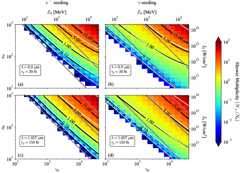
In Fig. 2, we report, as a function of and , the multiplicity () extracted from a set of 1D3V PIC simulations of electron-seeded (left panels) and photon-seeded (right panels) showers, for ultra-short (, ) pulses (top panels) and longer (, ) pulses (bottom panels). Each panel summarizes the results of simulations considering values of from to and values of from to (both axes discretized in logarithmic scale).
The white region in the bottom-left part of each panel corresponds to a low multiplicity regime (), that will not be much discussed here for two reasons. First, it is of marginal interest for forthcoming experiments on multi-petawatt laser systems, see Fig. 1. Second, it corresponds to a regime where the standard Monte-Carlo approach implemented in Smilei is not optimal (at least for systematic studies performed without consuming too much computer resources). Indeed, Monte-Carlo methods for the description of photon disintegration require a particle number greater than to ensure precision at level. As our simulations were performed with initial particles, the low multiplicity regime () is not well described.
The color-scaled region thus reports the number of produced pairs per incident particle, or multiplicity, as small as at moderate , and up to near a hundred at very large (top-right corner). Iso-contours of multiplicity , , , and are also reported: in black when extracted from our PIC simulations, and in white for the model predictions. For electron-seeded showers, a very good agreement is observed up to multiplicities of (not shown) and fair agreement for multiplicities of . For photon-seeded showers, a very good agreement is observed up to multiplicities of .
Before discussing the differences between electron- and photon seeding, as well as ultra-short (20 fs) and longer (150 fs) pulses,
let us note that the multiplicity iso-contours are not, in general, straight lines parallel to iso- (gray dotted) contours.
This means that is not the only parameter determining the total number of pairs,
and that by extension and do not play a symmetrical role in the shower development.
This was already discussed for the case of photon-seeded showers in [43],
and could have been expected from Eqs. (6) and (7)
where the rates depend on the incident particle energy as well as on its quantum parameter.
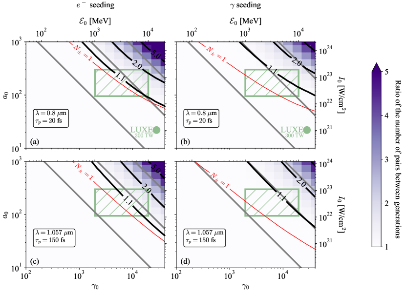
We are now in a position to discuss the model assumptions, namely the fact that we limit ourselves to a few generations and that to describe the energy evolution of the leptons we don’t need the full distribution function but we can limit ourselves to the first moment i.e. the average energy. In Fig. 3 we present (with the same hierarchy defined in Fig. 2) the final number of pairs divided by the number of pairs produced from the first (only for electron seeding) and the second (for photon seeding) generations extracted from PIC simulations. This plot acts as a definition of the regime of validity of our model where the black solid line (or the color map) corresponds to the iso-contour equal to and represents the error factor induced by the consideration of the first generations only. It is clear that for future experimental parameters, only a few generations of creation: first for electron seeding and first and second for photon seeding are enough to describe the number of pairs with at most an error of a factor .
Even if is not the only relevant parameter and because our results have a weak dependence on the pulse duration, at zero order, pair creation will not happen below a threshold of . Moreover as discussed in Fig. 3 our model is very well satisfied for less than . We can thus consider a simple argument to estimate the number of relevant generations [59]. If on average an initial electron with an initial energy of emits a photon with an energy of . This assumption holds for a large range of and is still approximately correct down to (the average energy varying from at to at ). The produced photon will create the first pair so that all its energy goes to one particle that will again emit a photon of energy . The reaction chain stopping for , we can infer that the initial value of consistent with one generation will be of the order of . For an initial photon at , the reasoning is similar. This photon decay to create one electron with the same energy and no one to the positron. Using the same intuitive result, the third generation starts for larger or order of . Even if all the parameters are not considered here, this simple estimation is in agreement with the full numerical analysis presented in Fig. 3 and allows us to get a rough estimate of the range of validity of the model.
The comparison between the model and PIC simulations shown in Fig. 2 proves that the average energy approximation gives a good estimation of the number of pairs. The initial particles are mono-energetic so at the beginning of the interaction the average energy is enough to describe the photon emission. After a certain cooling characteristic time, the spectrum also tends to a sharp Gaussian confirming the average approximation. During the transition regime, the spectrum is particularly broad but the average approximation still well describes the lower energetic photons emission. By using this hypothesis, we always underestimate the number of emitted photons with the energy of the order of their parent electron. This is a problem only in low multiplicity regimes () where the only photons capable of decay are those that have an energy near to their parent electron. Even if the model well predicts the scaling of the number we get an underestimation at low multiplicity. While in multiplicity order of , these rare photons do not influence the number of pairs because the decay process is mainly due to a high number of photons with lower energy. The average energy approximation allows first to take into account the energy conservation in the photon emission and second to describe these low energetic photons with a good precision giving an estimation in excellent agreement with simulations for moderate multiplicity (order of ) regime.
III.3 electron seeding vs photon seeding
Over the whole range of parameters studied here, we find that photon seeding always provides multiplicities larger or equal to those obtained using electron seeding. However, forthcoming experiments will likely produce a significantly larger number of GeV-level electrons than photons of similar energy. Apart from this practical consideration, it is interesting to explain the difference between electron and photon seeding. For clarity, we plot in Fig. 4(a) the multiplicity of pairs as a function of for , fs and m in the case of electron seeding (blue circles) and photon seeding (red squares). The black lines report our theoretical predictions obtained from Eq. (13) (for electron seeding) and Eqs. (18) and (21) (for photon seeding). The same quantity is shown as a function of for , fs and m in panel (b).
The largest difference between the two seeding strategies appears in the low multiplicity regime [ in Fig. 4(a) or in Fig. 4(b)] where the number of produced pairs per incident electron is significantly smaller than that obtained seeding the shower with photons. This can be easily explained as, in this regime, the seed electrons will emit many photons but with an energy significantly smaller than . Their quantum parameter will be much less than the quantum parameter associated to . The probability of these low-energy photons to decay will thus be significantly (exponentially) suppressed compared to the initial photon seeding case.
In contrast, in the large multiplicity regime, there is virtually no difference between seeding the shower with an electron or a photon beam at the same initial energy. A seed photon will quickly turn into a pair with one of the particles (either the electron or the positron)
carrying most of its energy, so the situation is very similar to seeding the shower with an electron beam.
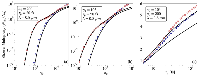
III.4 Ultra-short vs longer pulses
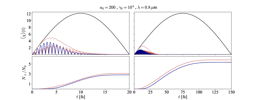
To illustrate the discussion, we show in Fig. 5 (top panel) the evolution of the quantum parameter of the incident electrons (in blue) or primary positrons (for photon seeding in red). Dashed red line represent in photon seeding case. On the bottom panel, we report the evolution of the multiplicity as a function of time in red for photons seeding and in blue for electrons seeding. In the case of a long pulse duration, the incident electrons dissipate their energy before reaching maximum intensity. As a result, the maximum average quantum parameters become less pronounced compared to a short-pulse case, and low-energy photon emission is favored. The competition between pair production rates over long and short periods can be succinctly characterized as follows: a set of low-energy photons interacting over a long duration versus a few high-energy photons interacting briefly. The nonlinearities of the proposed equations prevent a direct resolution of this question. Simulations reveal growth in the number of pairs with pulse duration throughout the parameter space explored see Fig. 4(c). However, for some excessive parameters not shown here, we saw that the number of pairs can decrease with the pulse duration. From this analysis, it is important to understand that at the same intensity increasing the total pulse duration (so the total energy) is not always favorable to pair production. Also, it is important to note that for a longer pulse, pairs will also lose their energy by radiation and then have more chance to bounce back. The detectors have to be set with this consideration and an explicit study of the bounce effect is studied in [60].
III.5 Comparison to previous models
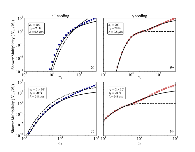
Calculations of the multiplicity in a similar configuration to the one considered here have been performed before by Blackburn et al. [42] for the electron seeding case and by Mercuri-Baron et al. [43] for the photon seeding one. In this section, we compare our results with these previous models and further discuss the different hypotheses in use and their validity.
In Fig. 6(a,b) we report the final number of pairs produced per incident particle as a function of the initial energy and [panels (a) and (b) for electron- and photon seeding, respectively]. In Fig. 6(c,d) we report the same quantity as a function of and fixed [panels (c) and (d) for electron- and photon seeding, respectively]. In all cases, the pulse parameters are fs and m. Red squares (photon seeding) and blue dots (electron seeding) are extracted from 1D3V PIC simulations. Our model predictions, Eq. (13) (electron seeding) or Eqs. (18) and (21) (photon seeding), are plotted as solid lines.
We first focus on electron seeding [panels (a) and (c)] and compare our predictions with those obtained using the model of Blackburn et al. [42], shown as black dotted lines. In that paper, to propose a completely analytical model, the authors performed several approximations: i) The expression of the rate and not the real probability is used for pair creation. This induces a systematic error when the multiplicity (or more accurately when ), leading to an overestimate of the number of produced pairs that, at high probability, can even overcome the number of available photons. ii) The nonlinear Compton Scattering rate is asymptotically expanded around . This is a very good assumption, as verified in our simulations, when the highest-energy photons are the ones responsible for pair creation, which is the case in the low-, low-multiplicity regime. However, as and the shower multiplicity increase, this approach fails in capturing the lower-energy photons that can contribute further to the pair production, and this assumption leads to underestimating the final number of final pairs. iii) The nonlinear Compton Scattering rate is evaluated at the initial electron energy and yet considering the time-dependent quantum parameter . This contrasts with our model (see Sec. II) we consistently evaluate the rate of photon emission using the time-dependent average energy and quantum parameter. iv) Finally, the number of pairs is calculated heuristically integrating (over energies) a function built as the product of the nonlinear Breit-Wheeler rate by the emitted photon energy distribution. This approach leads to another systematic overestimate of the number of produced pairs. In our work, we rather use the exact form given by Eq. (13) of this work.
Thanks to these approximations, Blackburn et al. obtain a fully analytical expression for the number of pairs produced in a shower driven by a linearly polarised Gaussian laser. Their prediction appears in fair agreement with simulations shown in Figs. 6 (a) and (c).
Our approach extends Blackburn’s by alleviating certain hypotheses that are not well justified in the regime of intermediate quantum parameters and potentially large shower multiplicities relevant to multi-petawatt laser facilities.
Doing so however requires a numerical integration of the main equations derived in Sec. II.2, but also allows for a more general treatment, not limited to the case of linearly polarized Gaussian beam.
Let us now turn our attention to the case of photon seeding. In Figs. 6(b) and (d) we show the prediction of the shower multiplicity obtained from the model of Mercuri-Baron et al. [43] (black dotted lines). In this case, the multiplicity is estimated by considering exactly one generation, i.e. assuming the soft-shower regime. The model is equivalent to Eq. eq18 and as we can see gives a very good agreement with simulations until the multiplicity becomes larger than . Note that in the work of [43], a fully analytical expression of Eq. 18 is given for arbitrary geometry (see also Appendix C).
In this work, we improve on the model of Mercuri-Baron et al. by computing the number of pairs of the second generation. Doing so extends the model of photon-seeded shower to multiplicities larger than 1, see Figs. 6 (a)-(d), and allows to cover the whole range of parameters relevant to forthcoming facilities.
To conclude, the models developed in Sec. II improve on previous works by Blackburn, Mercuri-Baron, and co-workers, and extend our prediction capabilities to multiplicities of the order of or larger than unity, relevant for multi-petawatt laser facilities. At very large values of , our models however underestimate the final number of pairs. This happens for multiplicities above typically 5, for which PIC simulations show that later generations of pairs and high-energy photons need to be accounted for. Such regimes of abundant pair production may not be easily accessible on near-feature facilities.
IV Three-dimensional effects & guidelines for future experiments
In this section, we generalize the model developed in Sec. II to account for three dimensions. The model predictions are then benchmarked against 3D3V PIC simulations. Finally, predictions for pair multiplicity under forthcoming experimental conditions are discussed.
IV.1 Three-dimensional model
To construct our three-dimensional model, we consider the head-on collision between a linearly polarized Gaussian laser pulse with beam waist (radius at in intensity) propagating in the -direction (henceforth referred to as the longitudinal direction) and an electron or gamma-photon beam propagating in the -direction. The latter (seed particle) beam has a characteristic longitudinal length and transverse size and is described, right before the collision, by its energy distribution function which we parameterize as follows:
| (22) |
Here denotes the position of the seed particles before the collision, stands for the seed particle beam density, and the transverse and longitudinal beam density profile normalized such that121212For a rectangular beam profile with transverse widths and one thus has . For a cylindrical beam with transverse radius , one has . and , and the beam energy distribution normalized such that . The total number of particles in the beam then reads .
The total number of pairs resulting from the collision can then be written in the form:
| (23) |
where measures the number of pairs produced by a single seed particle with energy initially located at and considering its full trajectory across the laser pulse.
To compute Eq. (23), we now introduce some assumptions on both the laser pulse and seed particle beam. As done for Sec. II, we first assume that all (seed and produced) particles move at ultra-relativistic speed along straight lines (see Sec. II.1 for details) so that the trajectories over which is computed are simple. We further assume that the laser and seed particle beams are perfectly synchronized and aligned131313That is, an ideal particle located at the center of the seeding beam and moving at the speed of light will reach the peak of the laser pulse at its focal plane. and that the characteristic (longitudinal) length of the seed particle beam is smaller than or at most of the order of the laser beam Rayleigh length and pulse length . This ensures that all seed particles within the focal spot can experience the laser field at its maximum and makes the integration over in Eq. (23) straightforward ( can then be taken independent of ). Under these assumptions, Eq. (23) can be rewritten:
| (24) |
Considering that pair production occurs mainly within the focal volume, the laser electromagnetic field is well approximated by simply multiplying Eq. (2) by a Gaussian dependency . As a result, is easily computed from the one-dimensional developed in Sec. II, using as given by Eq. (13) for electron-seeded showers, and with and given by Eqs. (18) and (21), respectively, for photon-seeded showers. Here, and are computed for all values of and using the laser field strength evaluated at .
In the limit of a thin seed-particle beam, , one can make the approximation in Eq. (24). The resulting number of produced pairs can then be simply extracted from the one-dimensional predictions of Sec. II:
| (25) |
In the limit of a broad (pancake-like) seed-particle beam, , one can take in Eq. (24) and the number of produced pairs can be computed as:
| (26) |
For this broad (pancake-like) seed-particle beam, we see that the electron beam is fully defined by its areal density and the total number of produced pairs is proportional to an effective, total cross-section (as introduced in Ref. [43]). It is interesting to rewrite Eq. (26) as , where is the number of seed particles in the focal volume and thus measures an effective multiplicity. For a Gaussian laser pulse, this effective multiplicity is independent of .
In what follows, we benchmark this three-dimensional model against self-consistent particle-in-cell simulations. As the case of a thin beam is a direct extrapolation of one-dimensional results, we rather focus our attention on the case of a pancake beam (). In addition, we now focus our attention on the case of a monochromatic seed-particle beam [].
IV.2 3D3V PIC simulations
In what follows we present 3D3V PIC simulations performed with Smilei. Each simulation reproduces a volume of (in the , and directions respectively) with spatial resolution and . Time resolution is set to . The laser propagates in the -direction and collides head-on with a counter-propagating beam of electrons or photons with finite longitudinal extension and an infinite transverse extension (periodic boundary conditions are used in the transverse direction). Each cell of the beam contains macro particles for a total of (seed) particles. The initial position of the particle beam is set so that if a particle at the center of the particle beam was always moving at , it would reach the peak intensity at the beam focus. The duration of the simulation is longer than the interaction time of the laser and the particles. All results presented hereafter have been extracted at the end of the simulations.
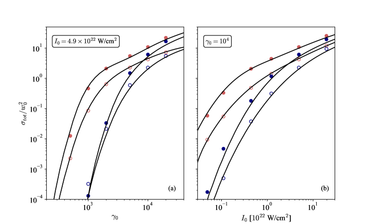
A set of simulations was performed considering the two types of laser facilities previously discussed, i.e. short Ti:Sapphire laser systems such as Apollon ( m and fs), and long Ne:Glass laser systems such as the ELI Beamlines A4 ATON ( m and fs). To compare the results on both types of facilities, results are presented as a function of the laser intensity (not field strength ). In addition, simulations have been performed using a fixed focusing aperture .
In Fig. 7, the resulting total cross sections (dots), in units of , are compared to those from the numerical integration of Eq. (26) (lines), as a function of and . Excellent agreement is observed for the range of parameters considered. Since the effect of finite transverse size is that many particles will interact with an intensity lower than the peak value , the approximation of considering only the first generation holds over a wider range of parameters in the three-dimensional case than in the one-dimensional limit. If we compare pulses with different duration and same field peak amplitude (here W/cm2 i.e. at m) it is interesting to notice that in the case of electron seeding, for the lowest electron energies we obtain a slightly larger cross-section for fs than fs. As discussed before, electrons lose more energy before reaching the peak of intensity in a long pulse, resulting in nonlinear Compton Scattering emitted photons with lower energy. This means that the number of pairs is not always a growing function of the pulse duration.
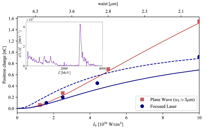
It is also interesting to compare the number of created pairs predicted by our model with previous self-consistent full-3D PIC simulations performed in Ref. [41]. As discussed in details below, the comparison shows excellent agreement and allows for quickly estimating the order of magnitude of expected pairs. The comparison is shown in Fig. 8. The pulse parameters are fs, m and the waist is variable in the different simulations (from 2 to 5 m corresponding to peak intensities from to W/cm2). The incident beam is generated by laser wake-field acceleration and contains approximately nC of GeV electrons. Considering only these particles, the density is C/cm3 with a longitudinal size of m. A first estimate can be obtained using Fig. 9 that reports our results with very similar laser parameters: . The positron charge is then nC, in excellent agreement with the nC obtained by full-3D PIC simulations in Ref. [41].
To obtain a more precise estimation, we extracted from their work the full energy spectrum of the incident electrons (shown in the inset panel of Fig.8) and performed the full calculation using Eq. (23). In Fig. 8, the red color stand for laser plane wave simulations with different intensities; the squares show the result of the 3D PIC simulation of [41] while the red line is obtained with Eq. (23). In this case the laser intensity does not depend on space and the parameters needed are the energy spectrum and the number of initial electrons. The calculation can then be performed in one dimension, and related to the multiplicity discussed in Sec. III.2. Notice that, in this case, the number of interacting electrons is kept constant and equal to the total number of electrons in the beam in the 3D simulations. The agreement with our calculation is excellent. Blue points are the results presented in Ref. [41] for a -J focused laser pulse with various spot sizes. The solid blue line corresponds to our prediction using Eq. (23) calculated with the full spatial distribution of the incident electron beam. We defined it as a cube of size m, m and m along and normal to the laser polarization and along the propagation direction, respectively. The cube is aligned with the focal spot. In this prediction, we neglected diffraction, meaning that the longitudinal geometry is not taken into account, but we still predict the final number of pairs within less than a factor . The dashed blue line shows our prediction for a pancake-like beam Eq. (26), considering a constant particle density (the number of interacting electrons increases with the waist). The trend is very similar to the case when the interaction is limited to the central spot, and as expected, for a waist of order or lower than the beam transverse size ( m) the results are in better agreement with the full 3D PIC simulation. Notice however that, even if the results of the pancake beam show a higher charge at large waist than the other two cases, a direct comparison in this range is not appropriate, since the total number of interacting electrons is not the same.
Finally, to guide future experiments we show in Fig. 9 the theoretical total cross-section normalized to for a pancake-like beam as a function of laser field intensity and initial incident energy for pulses like ELI and Apollon. A generalization to other situations can be found in [61]. In our case the cross section is proportional to and we present the value corresponding to an effective multiplicity. Thus, the number of created pairs after the interaction can be easily obtained as the number of incident particles initially in the waist times the effective multiplicity. In other words, a good estimation of the final number of pairs created can be calculated by: . If the initial beam is spread in energy, this formula can simply be multiplied by the initial energy spectrum and integrated over energies.
V Conclusions
In conclusion, we have developed a semi-analytical model that predicts the multiplicity of pair showers emerging from the head-on collision of high-energy seed particles (electrons or photons) with an ultra-high-intensity laser pulse. This model builds on previous works by Blackburn et al. [42] and Mercuri-Baron et al. [43] and extends their domain of validity to the regime of higher multiplicities and conditions relevant to forthcoming multi-petawatt laser facilities. The model follows the evolution of successive generations of high-energy photons and electron-positron pairs. It is shown that under conditions of interest for this study, that correspond nonetheless to a large range of laser field strengths and seed particle energies, only the first generations contribute to the shower while large multiplicities, in the range 1 to 15, can still be achieved. This result is confirmed by both one-dimensional and three-dimensional PIC simulations, and the model is used to draw guidelines for future experiments.
The difference between electron- and photon-seeded showers is clarified. In the regime of moderate quantum parameter, , small multiplicities are expected and photon seeding is significantly more favorable than electron seeding (as far as we are concerned with multiplicity and not absolute numbers of produced particles). At higher quantum parameters, and for higher multiplicities, both seeding strategies lead to equivalent multiplicities so that electron seeding can be expected to lead to a larger (absolute) number of produced pairs.
The effect of pulse duration (for a given peak intensity) is also discussed. At high intensities, relevant to forthcoming experiments at multi-petawatt laser facilities, pair production is weakly dependent on the interaction time. For long pulses, the primary particles mainly interact or lose energy in the initial part of the pulse and do not attain the maximum reachable quantum parameter. Contrary to what could be naively expected, we find that the number of produced pairs does not increase linearly with the pulse duration (nor energy). In practical terms, it means that, considering a similar maximum intensity for the laser pulse, the multiplicity of showers using long Nd:Glass laser is only marginally increased compared to what can be achieved using a short Ti:Sapphire laser.
Last we want to point out that, while this work focused on head-on collisions of high-energy electron or photon beams against linearly-polarised lasers with Gaussian (in space) and (in time) beam profile, our model — and in particular Eqs. (11), (13), (19), (18) and (21) — can be used considering arbitrary polarizations, spatio-temporal laser beam shapes and collision angles. Furthermore, while we discussed mainly monoenergetic and very thin (in the longitudinal direction) particle beams, extension to arbitrary energy and spatial distribution can be easily obtained.
Acknowledgements
The authors are grateful to E. Gelfer and S. Weber for fruitful discussions. This work used the open-source PIC code SMILEI, the authors are grateful to all SMILEI contributors and to the SMILEI-dev team for its support. Simulations were performed on the Irene-Joliot-Curie machine hosted at TGCC, France, using High-Performance Computing resources from GENCI-TGCC (Grant No. A0030507678). This work received financial support from the French state agency Agence Nationale de la Recherche, in the context of the Investissements d’Avenir program (reference ANR-18-EURE-0014). A.A.M. was supported by Sorbonne Université in the framework of the Initiative Physique des Infinis (IDEX SUPER). The work of T.G. and M.V. was supported by FCT grants: CEECIND/04050/2021, CEECIND/01906/2018 and PTDC/FISPLA/3800/2021.
Appendix A Governing equations for the full distribution functions
Placing ourselves within the locally-constant crossed field approximation (LCFA), neglecting particle acceleration in the laser field and any spatial non-uniformities, one can cast the cascade equations in the form:
| (27) | |||||
| (28) |
Equation (27) defines the dynamics of the energy distribution of electrons () and positrons (). The first two terms in the equation right-hand-side describe the effect of high-energy photon emission via nonlinear inverse Compton scattering on the electron/positron dynamics (radiation reaction). The last term describes the creation of new pairs by nonlinear Breit Wheeler and depends on photon distribution only. Finally, the evolution of the photon energy distribution () is given by Eq. (28). The first two terms account for the emission of new photons by electrons and positrons, respectively, and the last term corresponds to the decay of photons into new pairs.
The energy distribution functions , and as described by Eqs. (27) and (28) account for all electrons, positrons and photons independently of their origin. In this work, we have shown that it can be interesting to split each population in successive generations that may be treated separately. We define and the distribution function of electrons and positrons created by photons of the generation. Similarly, photons of the generation are those created by the generation of electrons and positrons, and their distribution function is denoted . From this definition, it is clear that the full distribution function of photons electron and positron can be reconstructed summing over all particle generations: with .
The equation evolution governing the generation distribution functions read:
| (29) | |||||
| (30) | |||||
A general solution of Eq. (30) can be obtained using the variation of parameter method, which gives:
| (31) |
with
| (32) |
Note that the term is non-zero only for generation in the case of a photon-seeded shower.
Integrating Eq. (29) over all charged particle energy () and interaction time leads the number of pairs generated at the generation:
| (33) |
Injecting Eq. (31) into (33) and integrating by part gives:
| (34) | |||||
The first term of this general expression can be intuited by considering that the creation of pairs at a given time corresponds to the probability to create a photon multiplied by the probability of this photon to decay during an interval of time equal to the difference of the given time and the photon creation time. This is expressed as a convolution of these two probabilities weighted by the distribution function of the parent charged particle.
The second term takes into account the generation of pairs by the initial () photons but is non-zero only for the particular case of photon seeding.
Let us finally note that, summing Eq. (34) over all successive generations, we obtain the total number of pairs as a function of the photon, electron, and positron distribution functions.
Appendix B Photon emission and pair production rates
Appendix C Number of primary pairs in photon-seeded cascades
In Ref. [43], the authors derive an analytical approximation for the number of primary pairs created in a photon-seeded shower. Considering head-on collision with a linearly polarized light pulse described by Eq. (2), it reads:
| (40) |
with
| (41) |
( denotes the integer part) denotes the number of half optical cycles a seed photon has experienced at a given time , and:
| (42) |
Here is the quantum parameter of a photon seeing the field extremum, computed considering a sin2 intensity envelope [see Eq. (2)], is the error function and with defined in Appendix B and its derivative.
References
- Bhabha and Heitler [1937] H. J. Bhabha and W. Heitler, The passage of fast electrons and the theory of cosmic showers, Proceedings of the Royal Society of London. Series A-Mathematical and Physical Sciences 159, 432 (1937).
- Carlson and Oppenheimer [1937] J. Carlson and J. Oppenheimer, On multiplicative showers, Physical Review 51, 220 (1937).
- Rossi and Greisen [1941] B. Rossi and K. Greisen, Cosmic-ray theory, Reviews of Modern Physics 13, 240 (1941).
- Di Piazza et al. [2012] A. Di Piazza, C. Müller, K. Hatsagortsyan, and C. H. Keitel, Extremely high-intensity laser interactions with fundamental quantum systems, Reviews of Modern Physics 84, 1177 (2012).
- Fedotov [2016] A. Fedotov, Quantum regime of laser-matter interactions at extreme intensities, arXiv preprint arXiv:1612.02038 (2016).
- Breit and Wheeler [1934] G. Breit and J. A. Wheeler, Collision of two light quanta, Physical Review 46, 1087 (1934).
- Schwinger [1951] J. Schwinger, On gauge invariance and vacuum polarization 10.1103/PHYSREV.82.664 (1951).
- Nikishov and Ritus [1964] A. I. Nikishov and V. I. Ritus, Quantum processes in the field of a plane electromagnetic wave and in a constant field 1, (1964).
- Ritus [1979] V. I. Ritus, Quantum effects in the interaction of elementary particles with an intense electromagnetic field, (1979).
- Goldreich and Julian [1969] P. Goldreich and W. H. Julian, Pulsar electrodynamics, The Astrophysical Journal 10.1086/150119 (1969).
- Harding and Lai [2006] A. K. Harding and D. Lai, Physics of strongly magnetized neutron stars, Reports on Progress in Physics 10.1088/0034-4885/69/9/R03 (2006).
- Uzdensky and Rightley [2014] D. A. Uzdensky and S. Rightley, Plasma physics of extreme astrophysical environments., Reports on Progress in Physics 10.1088/0034-4885/77/3/036902 (2014).
- Timokhin [2010] A. Timokhin, Time-dependent pair cascades in magnetospheres of neutron stars - i. dynamics of the polar cap cascade with no particle supply from the neutron star surface, Monthly Notices of the Royal Astronomical Society 10.1111/J.1365-2966.2010.17286.X (2010).
- Medin and Lai [2010] Z. Medin and D. Lai, Pair cascades in the magnetospheres of strongly magnetized neutron stars, Monthly Notices of the Royal Astronomical Society 10.1111/J.1365-2966.2010.16776.X (2010).
- Sarri et al. [2015] G. Sarri, K. Poder, J. Cole, W. Schumaker, A. D. Piazza, B. Reville, T. Dzelzainis, D. Doria, L. A. Gizzi, G. Grittani, S. Kar, C. H. Keitel, K. Krushelnick, S. Kuschel, S. Mangles, Z. Najmudin, N. Shukla, L. O. Silva, D. Symes, A. Thomas, M. Vargas, J. Vieira, and M. Zepf, Generation of neutral and high-density electron-positron pair plasmas in the laboratory, Nature Communications 10.1038/NCOMMS7747 (2015).
- Bahk et al. [2004] S.-W. Bahk, P. Rousseau, T. A. Planchon, V. Chvykov, G. Kalintchenko, A. Maksimchuk, G. Mourou, and V. Yanovsky, Generation and characterization of the highest laser intensities (10(22) w/cm2)., Optics Letters 10.1364/OL.29.002837 (2004).
- Danson et al. [2019] C. Danson, C. Haefner, J. Bromage, T. Butcher, J. Chanteloup, E. Chowdhury, A. Galvanauskas, L. Gizzi, J. Hein, D. Hillier, N. Hopps, Y. Kato, E. Khazanov, R. Kodama, G. Korn, R. Li, Y. Li, J. Limpert, J. Ma, C. Nam, D. Neely, D. Papadopoulos, R. Penman, L. Qian, J. Rocca, A. Shaykin, C. Siders, C. Spindloe, S. Szatmári, R. Trines, J. Zhu, P. Zhu, and J. Zuegel, Petawatt and exawatt class lasers worldwide, High Power Laser Science and Engineering 10.1017/HPL.2019.36 (2019).
- Papadopoulos et al. [2016] D. Papadopoulos, J. Zou, C. L. Blanc, G. Chériaux, P. Georges, F. Druon, G. Mennerat, P. Ramirez, L. Martin, A. Fréneaux, A. Beluze, N. Lebas, P. Monot, F. Mathieu, and P. Audebert, The apollon 10 pw laser: experimental and theoretical investigation of the temporal characteristics, High Power Laser Science and Engineering 10.1017/HPL.2016.34 (2016).
- Nam et al. [2018] C. H. Nam, J. H. Sung, H. W. Lee, J. W. Youn, and S. K. Lee, Performance of the 20 fs, 4 pw ti: sapphire laser at corels, in CLEO: Science and Innovations (Optica Publishing Group, 2018) pp. STu4O–3.
- [20] Extreme light infrastructure (ELI), https://eli-laser.eu.
- Bromage et al. [2019] J. Bromage, S. Bahk, I. Begishev, C. Dorrer, M. Guardalben, B. Hoffman, J. Oliver, R. Roides, E. Schiesser, M. J. S. Iii, M. Spilatro, B. Webb, D. Weiner, and J. Zuegel, Technology development for ultraintense all-opcpa systems, High Power Laser Science and Engineering 10.1017/HPL.2018.64 (2019).
- Hernandez-Gomez et al. [2010] C. Hernandez-Gomez, S. Blake, O. Chekhlov, R. Clarke, A. Dunne, M. Galimberti, S. Hancock, R. Heathcote, P. Holligan, A. Lyachev, P. Matousek, I. Musgrave, D. Neely, P. Norreys, I. Ross, Y. Tang, T. Winstone, B. Wyborn, and J. Collier, The vulcan 10 pw project 10.1088/1742-6596/244/3/032006 (2010).
- [23] Zettawatt-equivalent ultrashort pulse laser system (ZEUS), https://zeus.engin.umich.edu.
- Yoon et al. [2021] J. W. Yoon, Y. G. Kim, I. W. Choi, J. H. Sung, H. W. Lee, S. K. Lee, and C. H. Nam, Realization of laser intensity over 10 23 w/cm 2, Optica 10.1364/OPTICA.420520 (2021).
- Chen et al. [2009] H. Chen, S. Wilks, J. D. Bonlie, E. Liang, J. Myatt, D. Price, D. D. Meyerhofer, and P. Beiersdorfer, Relativistic positron creation using ultraintense short pulse lasers., Physical Review Letters 10.1103/PHYSREVLETT.102.105001 (2009).
- Ridgers et al. [2012] C. Ridgers, C. S. Brady, R. Duclous, J. G. Kirk, K. Bennett, T. Arber, A. P. L. Robinson, and A. R. Bell, Dense electron-positron plasmas and ultraintense rays from laser-irradiated solids., Physical Review Letters 10.1103/PHYSREVLETT.108.165006 (2012).
- Liang et al. [2015] E. Liang, T. Clarke, A. Henderson, W. Fu, W. Lo, D. Taylor, P. Chaguine, Z. Shaochuan, Y. Hua, X. Cen, X. Wang, J. Kao, H. Hasson, G. Dyer, K. Serratto, N. Riley, M. E. Donovan, and T. Ditmire, High e+/e- ratio dense pair creation with 10 21 w.cm laser irradiating solid targets, Scientific Reports 10.1038/SREP13968 (2015).
- Zhu et al. [2016] X.-L. Zhu, T.-P. Yu, Z.-M. Sheng, Y. Yin, I. C. E. Turcu, and A. Pukhov, Dense gev electron-positron pairs generated by lasers in near-critical-density plasmas., Nature Communications 10.1038/NCOMMS13686 (2016).
- Zi et al. [2023] M. Zi, Y. Ma, X. Yang, G. B. Zhang, J. Liu, Y. Yuan, M. Peng, Y. Cui, and S. Kawata, Ultraintense and ultrashort laser fields high-energy – density positron and g-photon generation via two counter-propagating ultra-relativistic laser irradiating a solid target, (2023).
- Bell and Kirk [2008] A. R. Bell and J. G. Kirk, Possibility of prolific pair production with high-power lasers, Physical Review Letters 10.1103/PHYSREVLETT.101.200403 (2008).
- Kirk et al. [2009] J. G. Kirk, A. R. Bell, and I. Arka, Pair production in counter-propagating laser beams, Plasma Physics and Controlled Fusion 10.1088/0741-3335/51/8/085008 (2009).
- Fedotov et al. [2010] A. Fedotov, N. B. Narozhny, G. Mourou, and G. Korn, Limitations on the attainable intensity of high power lasers., Physical Review Letters 10.1103/PHYSREVLETT.105.080402 (2010).
- Elkina et al. [2011] N. V. Elkina, A. Fedotov, I. Y. Kostyukov, M. V. Legkov, N. B. Narozhny, E. N. Nerush, and H. Ruhl, Qed cascades induced by circularly polarized laser fields, Physical Review Special Topics-accelerators and Beams 10.1103/PHYSREVSTAB.14.054401 (2011).
- Gelfer et al. [2015] E. G. Gelfer, A. A. Mironov, A. Fedotov, V. F. Bashmakov, E. N. Nerush, I. Y. Kostyukov, and N. B. Narozhny, Optimized multibeam configuration for observation of qed cascades, Physical Review A 10.1103/PHYSREVA.92.022113 (2015).
- Grismayer et al. [2016] T. Grismayer, M. Vranic, J. L. Martins, R. Fonseca, and L. O. Silva, Laser absorption via quantum electrodynamics cascades in counter propagating laser pulses, Physics of Plasmas 10.1063/1.4950841 (2016).
- Jirka et al. [2017] M. Jirka, O. Klimo, M. Vranic, S. Weber, and G. Korn, Qed cascade with 10 pw-class lasers, Scientific Reports 10.1038/S41598-017-15747-1 (2017).
- Vranic et al. [2017] M. Vranic, T. Grismayer, R. Fonseca, and L. O. Silva, Electron–positron cascades in multiple-laser optical traps, Plasma Physics and Controlled Fusion 10.1088/0741-3335/59/1/014040 (2017).
- Gonoskov et al. [2017] A. Gonoskov, A. Bashinov, S. Bastrakov, E. Efimenko, A. Ilderton, A. Kim, M. Marklund, I. Meyerov, A. Muraviev, and A. Sergeev, Ultrabright gev photon source via controlled electromagnetic cascades in laser-dipole waves, Physical Review X 7, 041003 (2017).
- Burke et al. [1997] D. Burke, R. Field, G. Horton-Smith, J. Spencer, D. Walz, S. Berridge, W. Bugg, K. Shmakov, A. Weidemann, C. Bula, et al., Positron production in multiphoton light-by-light scattering, Physical Review Letters 79, 1626 (1997).
- Mironov et al. [2016] A. Mironov, A. Fedotov, and N. Narozhny, Generation of quantum-electrodynamic cascades in oblique collisions of ultrarelativistic electrons with an intense laser field 10.1070/QEL16057 (2016).
- Lobet et al. [2017] M. Lobet, X. Davoine, E. d’Humières, and L. Gremillet, Generation of high-energy electron-positron pairs in the collision of a laser-accelerated electron beam with a multipetawatt laser, Physical Review Accelerators and Beams 20, 043401 (2017).
- Blackburn et al. [2017] T. Blackburn, A. Ilderton, C. Murphy, and M. Marklund, Scaling laws for positron production in laser–electron-beam collisions, Physical Review A 96, 022128 (2017).
- Mercuri-Baron et al. [2021] A. Mercuri-Baron, M. Grech, F. Niel, A. Grassi, M. Lobet, A. Di Piazza, and C. Riconda, Impact of the laser spatio-temporal shape on breit–wheeler pair production, New Journal of Physics 23, 085006 (2021).
- Golub et al. [2022] A. Golub, S. Villalba-Chávez, and C. Müller, Nonlinear breit-wheeler pair production in collisions of bremsstrahlung quanta and a tightly focused laser pulse, Physical Review D 105, 116016 (2022).
- Yu et al. [2019] J. Q. Yu, H. Lu, T. Takahashi, R. Hu, Z. Gong, W. Ma, Y. Huang, C. E. Chen, and X. Yan, Creation of electron-positron pairs in photon-photon collisions driven by 10-pw laser pulses., Physical Review Letters 10.1103/PHYSREVLETT.122.014802 (2019).
- Martinez et al. [2023] B. Martinez, B. Barbosa, M. Vranic, B. Martinez, B. Barbosa, and M. Vranic, Creation and direct laser acceleration of positrons in a single stage 10.1103/PHYSREVACCELBEAMS.26.011301 (2023).
- Grismayer et al. [2017] T. Grismayer, M. Vranic, J. L. Martins, R. Fonseca, and L. O. Silva, Seeded qed cascades in counterpropagating laser pulses., Physical Review E 10.1103/PHYSREVE.95.023210 (2017).
- Luo et al. [2018] W. Luo, W.-Y. Liu, T. Yuan, M. Chen, J.-Y. Yu, F. Li, D. D. Sorbo, C. Ridgers, and Z.-M. Sheng, Qed cascade saturation in extreme high fields., Scientific Reports 10.1038/S41598-018-26785-8 (2018).
- Bulanov et al. [2013] S. Bulanov, C. Schroeder, E. Esarey, and W. Leemans, Electromagnetic cascade in high-energy electron, positron, and photon interactions with intense laser pulses, Physical Review A 10.1103/PHYSREVA.87.062110 (2013).
- Mironov et al. [2014] A. A. Mironov, N. B. Narozhny, and A. Fedotov, Collapse and revival of electromagnetic cascades in focused intense laser pulses, Physics Letters A 10.1016/J.PHYSLETA.2014.09.058 (2014).
- Derouillat et al. [2018] J. Derouillat, A. Beck, F. Perez, T. Vinci, M. Chiaramello, A. D. Grassi, M. Flé, G. Bouchard, I. Plotnikov, N. Aunai, J. Dargent, C. Riconda, and M. Grech, Smilei : A collaborative, open-source, multi-purpose particle-in-cell code for plasma simulation 10.1016/J.CPC.2017.09.024 (2018).
- Duclous et al. [2011] R. Duclous, J. G. Kirk, and A. Bell, Monte carlo calculations of pair production in high-intensity laser–plasma interactions 10.1088/0741-3335/53/1/015009 (2011).
- Arber et al. [2015] T. Arber, K. Bennett, C. Brady, A. Lawrence-Douglas, M. Ramsay, N. Sircombe, P. Gillies, R. Evans, H. Schmitz, A. Bell, and C. Ridgers, Contemporary particle-in-cell approach to laser-plasma modelling 10.1088/0741-3335/57/11/113001 (2015).
- Gonoskov et al. [2015] A. Gonoskov, S. I. Bastrakov, E. Efimenko, A. Ilderton, M. Marklund, I. B. Meyerov, A. Muraviev, A. M. Sergeev, I. A. Surmin, and E. Wallin, Extended particle-in-cell schemes for physics in ultrastrong laser fields: Review and developments, Physical Review E 10.1103/PHYSREVE.92.023305 (2015).
- Vranic et al. [2015] M. Vranic, T. Grismayer, J. L. Martins, R. Fonseca, and L. O. Silva, Particle merging algorithm for pic codes, Computer Physics Communications 10.1016/J.CPC.2015.01.020 (2015).
- Lobet et al. [2016] M. Lobet, E. d’Humières, M. Grech, C. Ruyer, X. Davoine, and L. Gremillet, Modeling of radiative and quantum electrodynamics effects in pic simulations of ultra-relativistic laser-plasma interaction, Journal of physics 10.1088/1742-6596/688/1/012058 (2016).
- Niel [2021] F. Niel, Classical and quantum description of plasma and radiation in strong fields (Springer Nature, 2021).
- Baier et al. [1998] V. N. Baier, V. M. Katkov, and V. M. Strakhovenko, Electromagnetic processes at high energies in oriented single crystals (World Scientific, 1998).
- Akhiezer et al. [1994] A. Akhiezer, N. Merenkov, and A. Rekalo, On a kinetic theory of electromagnetic showers in strong magnetic fields, Journal of Physics G: Nuclear and Particle Physics 20, 1499 (1994).
- Qu et al. [2022] K. Qu, S. Meuren, and N. J. Fisch, Collective plasma effects of electron–positron pairs in beam-driven qed cascades, Physics of Plasmas 29, 042117 (2022).
- Amaro and Vranic [2021] Ó. Amaro and M. Vranic, Optimal laser focusing for positron production in laser–electron scattering, New Journal of Physics 23, 115001 (2021).