Multiscale dimension reduction for flow and transport problems in thin domain with reactive boundaries
Abstract
In this paper, we consider flow and transport problems in thin domains. Modeling problems in thin domains occur in many applications, where thin domains lead to some type of reduced models. A typical example is one dimensional reduced-order model for flows in pipe-like geometries (e.g., blood vessels). In many reduced-order models, the model equations are described apriori by some analytical approaches. In this paper, we propose the use of multiscale methods, which are alternative to reduced-order models and can represent reduced-dimension modeling by using fewer basis functions (e.g., the use of one basis function corresponds to one dimensional approximation).
The mathematical model considered in the paper is described by a system of equations for velocity, pressure, and concentration, where the flow is described by the Stokes equations, and the transport is described by an unsteady convection-diffusion equation with non-homogeneous boundary conditions on walls (reactive boundaries). We start with the finite element approximation of the problem on unstructured grids and use it as a reference solution for two and three-dimensional model problems. Fine grid approximation resolves complex geometries on the grid level and leads to a large discrete system of equations that is computationally expensive to solve. To reduce the size of the discrete systems, we develop a multiscale model reduction technique, where we construct local multiscale basis functions to generate a lower-dimensional model on a coarse grid. The proposed multiscale model reduction is based on the Discontinuous Galerkin Generalized Multiscale Finite Element Method (DG-GMsGEM). In DG-GMsFEM for flow problems, we start with constructing the snapshot space for each interface between coarse grid cells to capture possible flows. For the reduction of the snapshot space size, we perform a dimension reduction via a solution of the local spectral problem and use eigenvectors corresponding to the smallest eigenvalues as multiscale basis functions for the approximation on the coarse grid. For the transport problem, we construct multiscale basis functions for each interface between coarse grid cells and present additional basis functions to capture non-homogeneous boundary conditions on walls. Finally, we will present some numerical simulations for three test geometries for two and three-dimensional problems to demonstrate the method’s performance.
1 Introduction
Mathematical models in thin domains occur in many real-world applications, scientific and engineering problems. Fluid flow and transport in thin tube structures are widely used in biological applications, for example, to simulate blood flow in vessels [1, 2, 3]. In engineering problems, flow simulation is used to study fluid flow in complex pipe structures, for example in pipewise industrial installations, wells in oil and gas industry, heat exchangers, etc. In reservoir simulations, thin domains are related to the fractures that usually have complex geometries with very small thickness compared to typical reservoir sizes [4, 5, 6]. Such problems are often considered with complex interaction processes with surrounding media or walls. In many applications, these problems are transformed to reduced (e.g., one) dimensional problems via some type of apriori postulated models. Our goal is to present an alternative approach to analytical model reduction by using multiscale basis functions.
For the applicability of the convenient numerical methods for simulations of such problems, a very fine grid should be constructed to resolve the geometry’s complex structure on the grid level. Moreover, a very small domain thickness provides an additional complexity in the grid construction for thin and long domains. For a fast and accurate solution of the presented problem, a homogenization (upscaling) technique or multiscale models are used, which are based on constructing the lower dimensional coarse grid models. The asymptotic behavior of the solutions in thin domains is intensively studied. In [7], the authors consider the problem of complete asymptotic expansion for the time-dependent Poiseuille flow in a thin tube. In [8], the method of asymptotic partial decomposition of a domain (MAPDD) was presented to reduce the computational complexity of the numerical solution of such problems. This method combines the three-dimensional description in some neighborhoods of bifurcations and the one-dimensional description out of these small subdomains, and it prescribes some special junction conditions at the interface between these 3D and 1D submodels. Numerical results were presented in [2] for the method of asymptotic partial domain decomposition for thin tube structures with Newtonian and non-Newtonian flows in large systems of vessels. Our goal is to provide an alternative systematic approach to model reduction for thin domain problems that can add complexity via additional multiscale basis functions.
Model reduction techniques usually depend on a coarse grid approximation, which can be obtained by discretizing the problem on a coarse grid and choosing a suitable coarse-grid formulation of the problem. In the literature, several approaches have been developed to obtain the coarse-grid formulation for the problems in heterogeneous domains, including multiscale finite element method [9, 10, 11], mixed multiscale finite element method [12, 13], generalized multiscale finite element method [14, 15, 16, 17, 18], multiscale mortar mixed finite element method [19], multiscale finite volume method [20, 21], variational multiscale methods [22, 23, 24], and heterogeneous multiscale methods [25] and etc. The non - conforming multiscale method is considered for the solution of the Stokes flow problem in a heterogeneous domain in [26, 27]. In [28, 29], we presented the Generalized Multiscale Finite Element Method (GMsFEM) for the solution of the flow problems in perforated domains with continuous multiscale basis functions. GMsFEM shows a good accuracy for solving the nonlinear (non - Newtonian) fluid flow problems [30]. In [31], we presented the Discontinuous Galerkin Generalized Multiscale Finite Element Method (DG-GMsFEM) for the solving the two - dimensional problems in perforated domains.
In this paper, we consider flow and transport processes in thin structures with reactive boundaries. The mathematical model is described using Stokes equations and the unsteady convection-diffusion equation with non - homogeneous boundary conditions. Non-homogeneous boundary conditions occur in many applications. For example, the pore-scale modeling and simulation of reactive flow in porous media have many applications in many branches of science such as biology, physics, chemistry, geomechanics, and geology [32, 33, 34]. In order to handle the complex geometry of the walls and non-homogeneous boundary conditions on them, we present additional spectral multiscale basis functions. In this work, we continue developing the multiscale model reduction techniques for problems with multiscale features and developing the generalization of the techniques for DG-GMsFEM. In our previous work [35, 36], we considered elliptic problems in perforated domains and constructed additional basis functions to capture non-homogeneous boundary conditions on perforations. In [35], we proposed a non-local multi-continua (NLMC) method for Laplace, elasticity, and parabolic equations with non-homogeneous boundary conditions on perforations. In [36], we considered the Continuous Galerkin Generalized Multiscale Finite Element Method (CG-GMsFEM) for problems in perforated domains with non-homogeneous boundary conditions, where we constructed one additional basis function for local domains with perforations. Recently, we extended this technique for solving unsaturated flow problems in heterogeneous domains with rough boundary [37]. In this work, we consider DG-GMsFEM and present additional spectral basis functions for rough non-homogeneous boundaries in transport problems. The concept is based on the separation of the snapshots for each feature and shares a lot of similarities with multiscale methods for fractured media presented in our previous works [38, 39]. Our work is also motivated by a recently developed Edge GMsFEM, where multiscale basis functions are constructed for each coarse grid interface [40, 41].
In this work, we use the DG-GMsFEM for constructing multiscale basis functions for problems in thin domains. The goals of this paper are in constructing the general approach for problems in complex thin geometries with an accurate approximation of the velocity space and transport processes. We construct local multiscale basis functions to generate a lower-dimensional model on a coarse grid. In DG-GMsFEM for flow problem, we start with constructing the snapshot space that captures possible flows between coarse cell interfaces. After constructing the snapshot space, we perform a dimension reduction by a solution of the local spectral problems. For the pressure approximation, we use piecewise constant functions on the coarse grid. For the transport problem, we construct multiscale basis functions for each interface between coarse grid cells and present additional basis functions to capture non-homogeneous boundary conditions on walls. The presented snapshot spaces can accurately capture processes on the rough wall boundaries with non-homogeneous boundary conditions on them. We present the results of the numerical simulations for three test geometries for two and three-dimensional problems.
As we mentioned earlier, our goal is to investigate the use of multiscale and generalized multiscale methods for dimension reduction for problems in this domains. Many existing approaches propose analytical or semi-analytical reduced-dimensional problems, where the dimensions are determined apriori. Our idea is to use generalized multiscale method and identify the dimension. The proposed approach combined with aposteriori error estimate can further identify the dimension across thin layers and allow obtaining more accurate solution.
The paper is organized as follows. In Section 2, we describe the problem formulation and the fine-scale approximation. In Section 3, we present the multiscale method for flow and transport processes in thin structures with rough reactive boundaries. In Section 4, we present numerical results. The paper ends with a conclusion.
2 Problem formulation
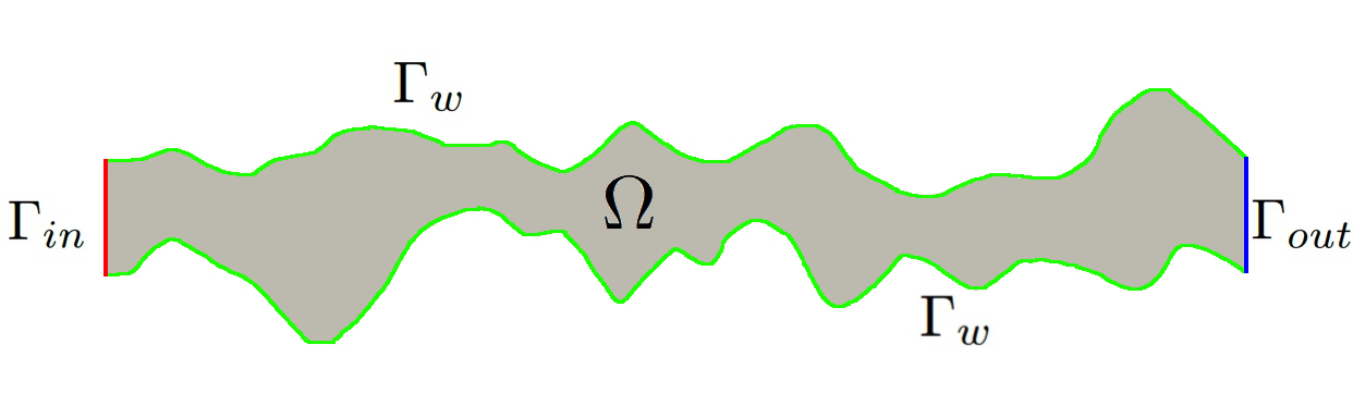
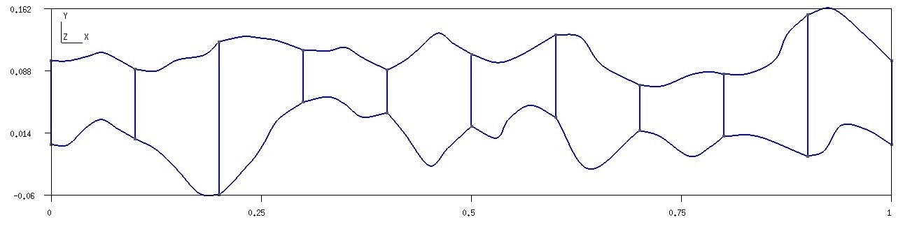
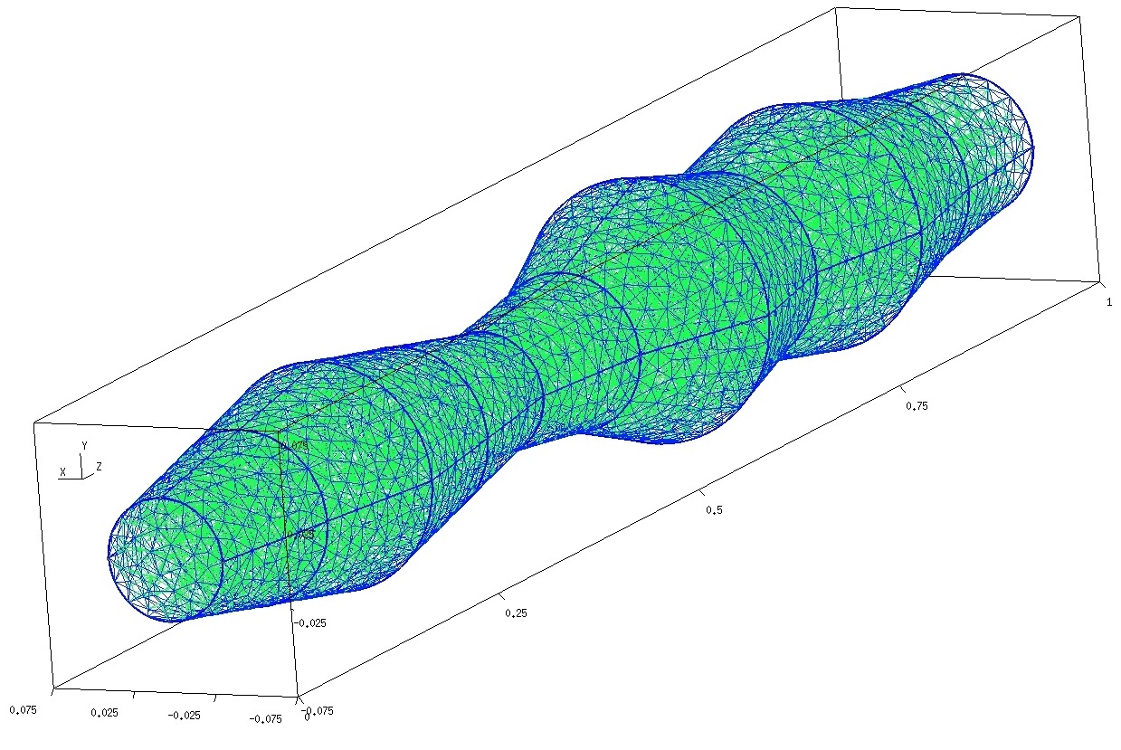
Let be a thin domain with multiscale features, where the thickness is small compared to the domain length (See Figure 1 for an illustration). We will consider the following flow and transport equations in the thin domain
| (1) |
where is the fluid viscosity, is the fluid density, is the diffusion coefficient, is the concentration, and are the velocity and pressure.
The system (1) is equipped with following initial conditions
Moreover, We consider the following boundary conditions for the flow problem
and for the transport problem
where is the unit outward normal vector on , is the identity matrix, is the inflow boundary, is the outflow boundary, is the reactive boundary of the thin domain, (see Figure 1).
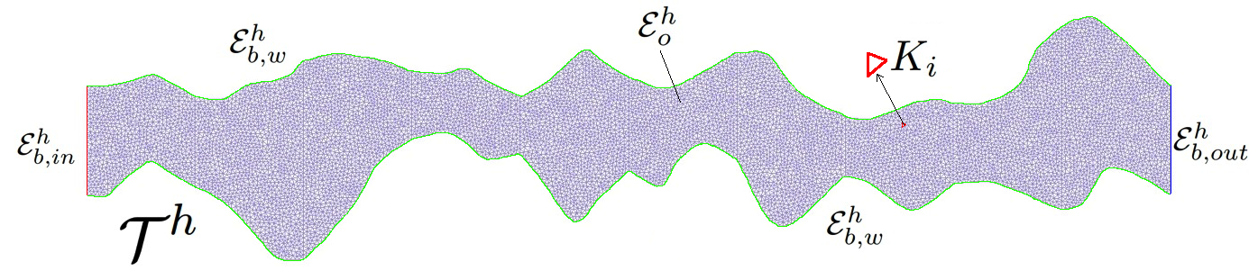
In order to solve the problem (1), we generate an unstructured grid (fine grid) and use a finite element approximation for the spatial discretization. Let be a fine-grid partition of the domain given by
where is the number of fine grid cells. We use to denote the set of facets in with , where is the set of interior facets and is the set of boundary facets with (see Figure 2). We use the notations and to denote a generic cell and facet in the fine grid (see Figure 2). We define the jump and the average of a function on interior facet by
where , , and are the two cells sharing the facet . Note that, we define and for .
We define the fine-scale velocity space
which contains functions that are piecewise linear in each fine-grid element and are discontinuous across coarse grid edges. For the pressure, we use the space of piecewise constant functions
The fine-scale space for concentration is the following
Using these spaces, we have the following IPDG variational formulation with implicit time approximation for the approximation of (1):
-
•
Flow problem: find such that
(2) where
and is the penalty perm.
-
•
Transport problem: find such that
(3) where
and is the penalty perm and .
In the above systems (2) and (3), and are the solutions from the previous time step and is the given time step size.
We can write the above discrete systems (2) and (3) as follows.
-
•
Flow problem:
(4) -
•
Transport problem:
(5) Here, the matrix depends on the function .
In the next section, we will present the proposed multiscale method for the solution of the flow and transport problems that used to reduce the system size. In the multiscale method, we solve problems in local domains with various boundary conditions to form a snapshot space and use a spectral problem in the snapshot space to perform the required dimension reduction.
3 Multiscale method
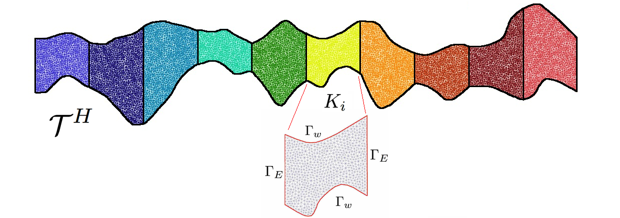
Let be a coarse-grid partition of the domain with mesh size (see Figure 3)
where is the number of coarse grid cells (local domains). We use to denote the set of facets in with . For the construction of the coarse grid approximation, we use the Discontinuous Galerkin Generalized Multiscale Finite Element Method (DG-GMsFEM). In DG-GMsFEM, the multiscale basis functions are supported in each coarse cell [28, 29, 31]. We define as the multiscale velocity space and as the multiscale space for concentration. For the pressure approximation, we use the piecewise constant function space over the coarse cells.
We denote the multiscale spaces for concentration and velocity as
respectively, where is the number of basis functions for velocity, is the number of basis functions for concentration. For the pressure, we use the space of piecewise constant functions over the coarse grid cells
where is equal to the number of coarse grid cells ().
For the coarse grid approximation, we have the following variational formulation:
-
•
Flow problem: find such that
(6) -
•
Transport problem: find such that
(7)
Next, we consider the construction of the multiscale basis functions for velocity and concentration.
3.1 Multiscale space for velocity
For the construction of the multiscale space for the velocity, we start with the construction of the snapshot space. The snapshot space is formed by the solution of local problems with all possible boundary conditions up to the fine grid resolution in each coarse cell , where is the number of coarse blocks in . After that, we solve a local spectral problem to select dominant modes of the snapshot space.
We consider two types of multiscale spaces:
-
•
Type 1. Multiscale space for flow is defined so that snapshot spaces and spectral problems are constructed for all flow directions.
-
•
Type 2. Multiscale space for flow is defined so that snapshot spaces and spectral problems are constructed separately for each flow direction.
We start with the construction of the Type 2 multiscale basis functions. The local snapshot space consists of functions which are solutions of the following problem
| (8) | |||||
with boundary conditions
for , is the number of fine grid facets on , and is the vector discrete delta function defined on , is the interface between local domains ( and is dimension of problem). Here constant is chosen by the compatibility condition, . For 2D problem, we solve local problems (8) using the following
For 3D problem, we solve the local problems (8) using the following
In the above, is the discrete delta function whose value is on the -th fine grid node and otherwise. We remark that the local problems (8) are solved on the fine mesh by using a standard numerical scheme. Using these local solutions, we form the following local snapshot space
where the flow direction, , are considered separately.
To reduce the size of direction based snapshot spaces, we solve following local spectral problem in each snapshot space in
| (9) |
where
and is the matrix representation of the bilinear form and is the matrix representation of the bilinear form
| (10) |
The above snapshot space projection matrix is defined by collecting all local solutions
We remark that the integral in is defined on the boundary of the coarse block, and is the fine grid for local domain .
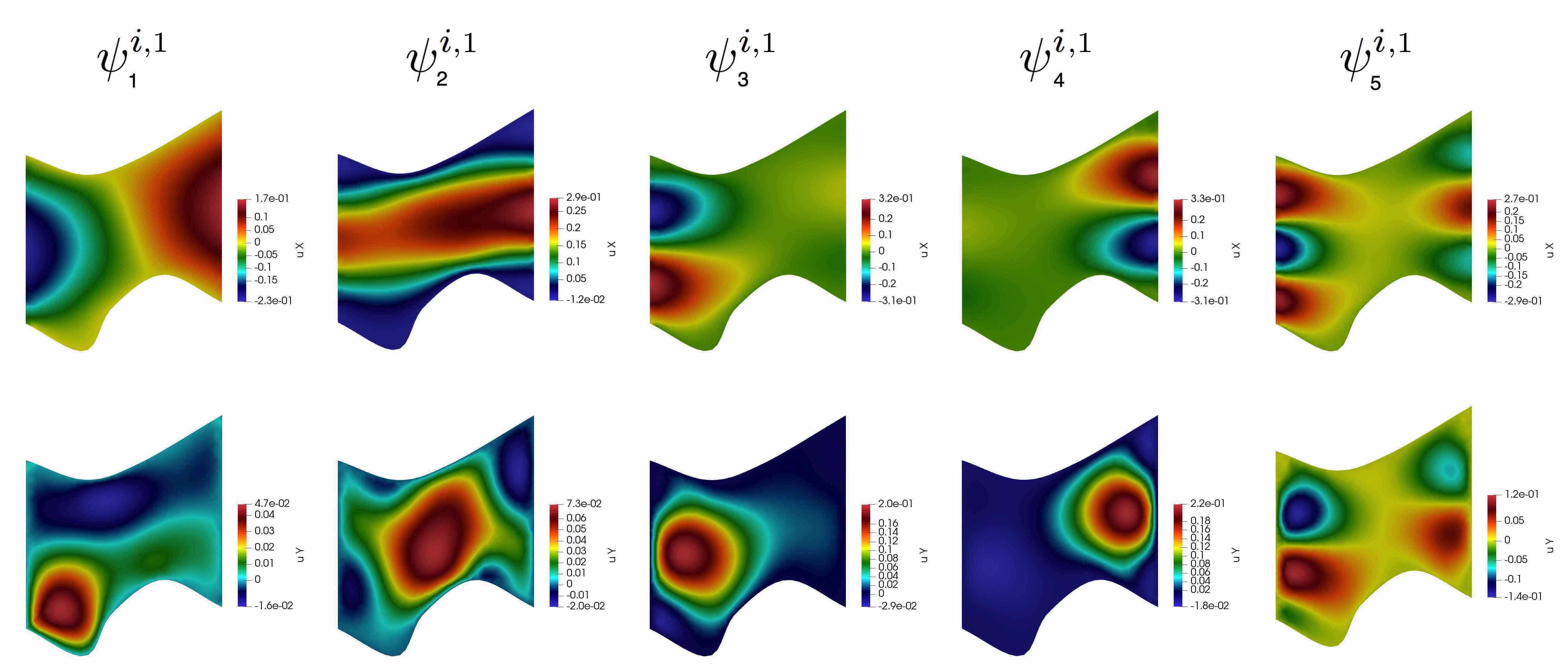
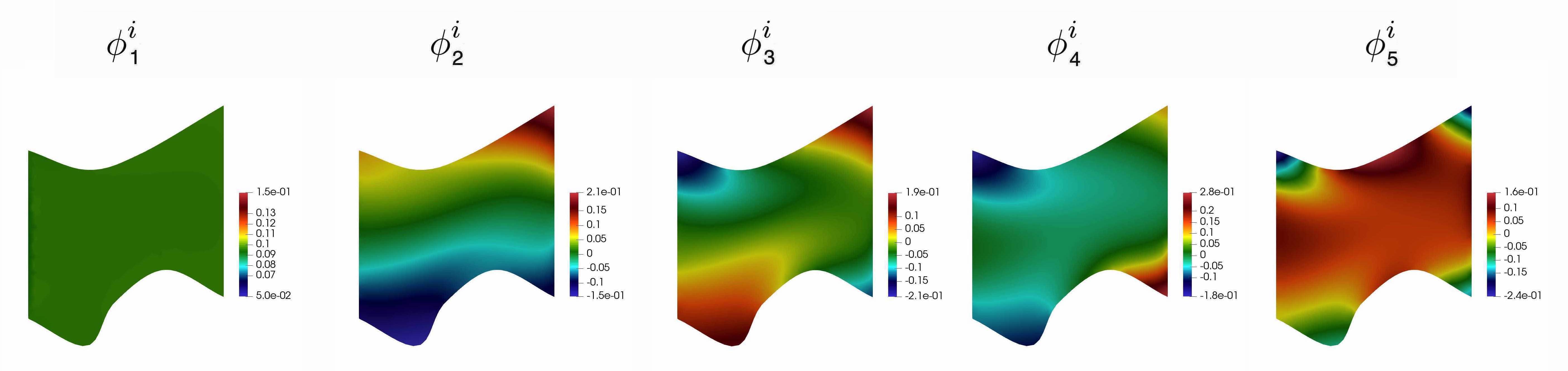
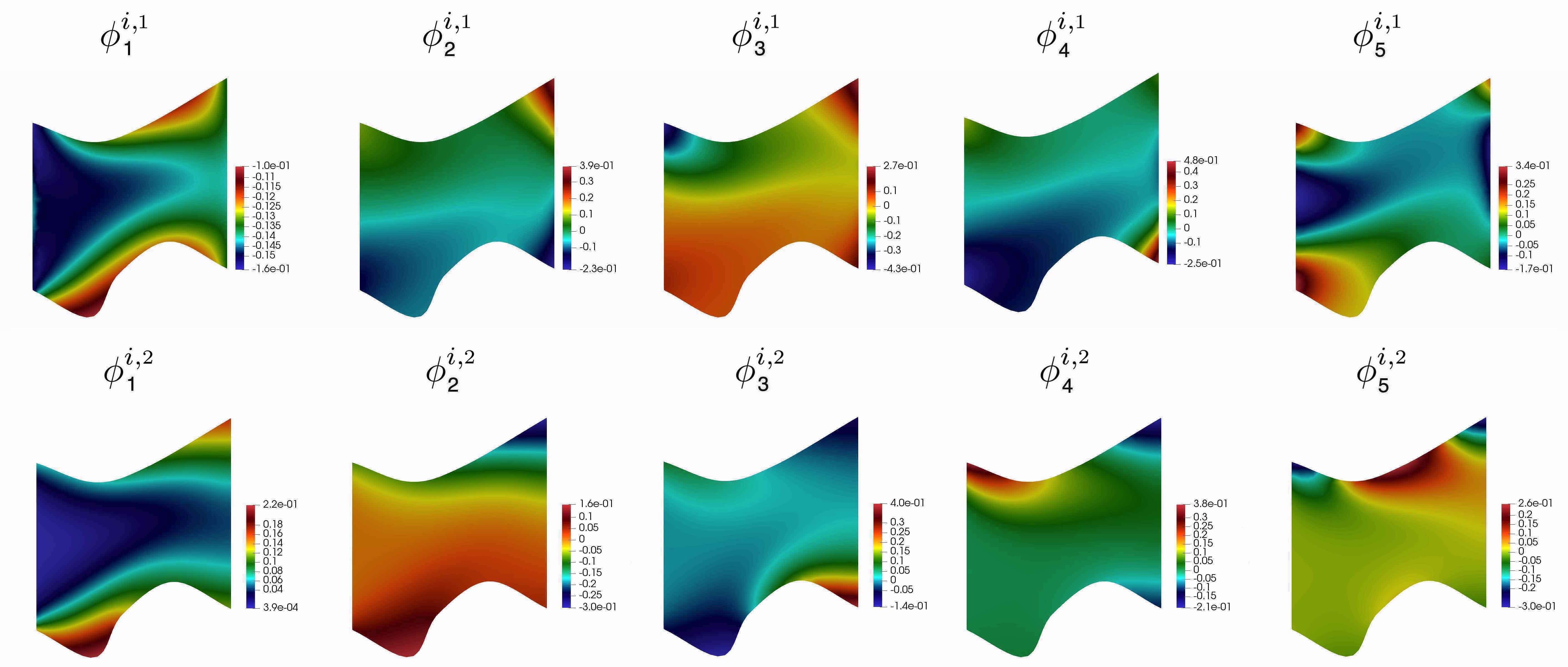
To form a direction based multiscale space for velocity, we arrange the eigenvalues in increasing order and choose eigenvectors corresponding to the first the smallest eigenvalues for each flow direction
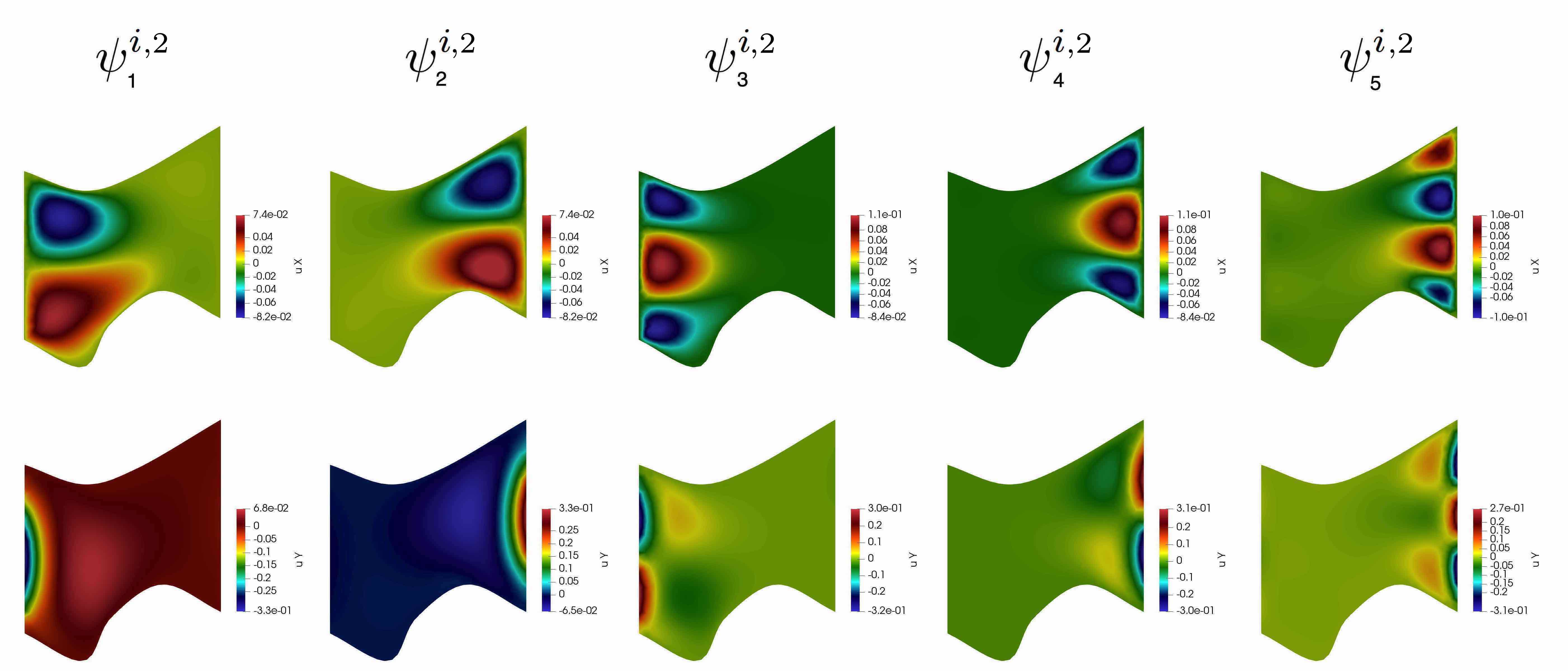
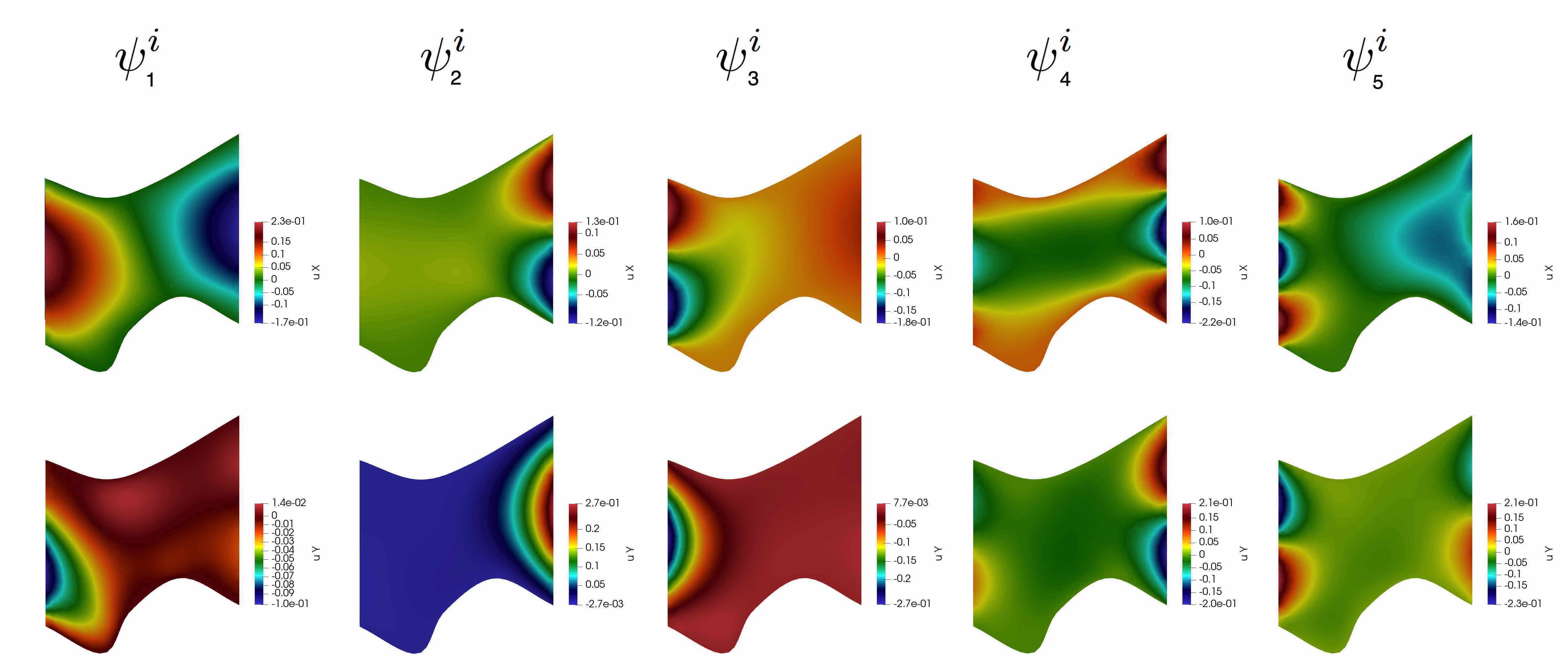
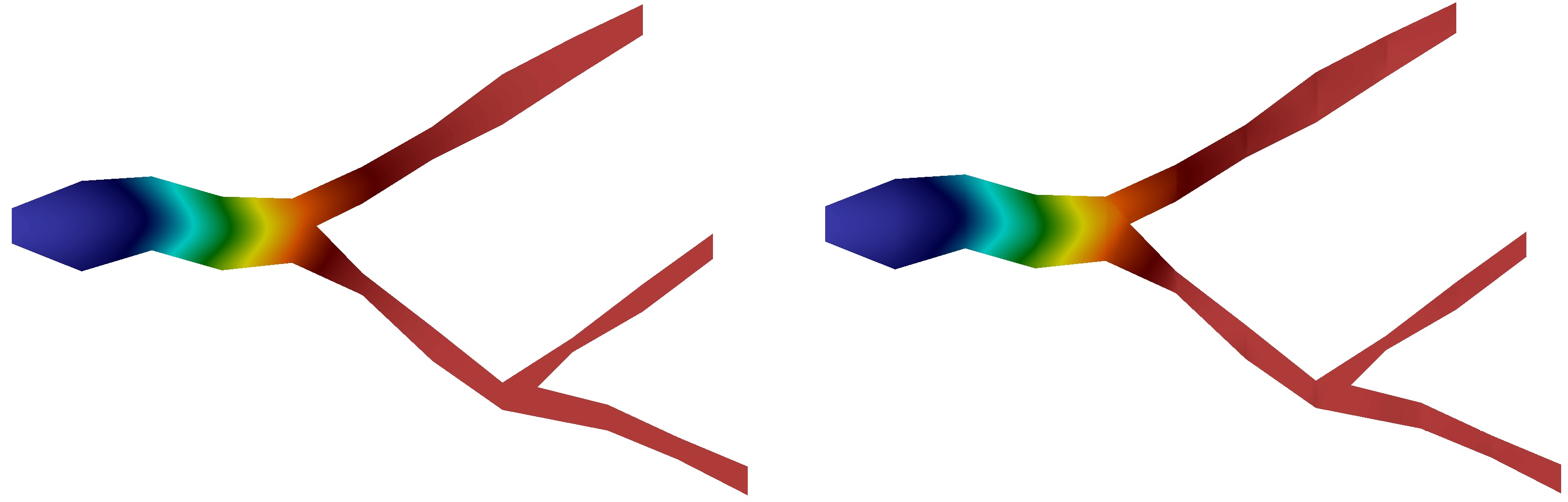
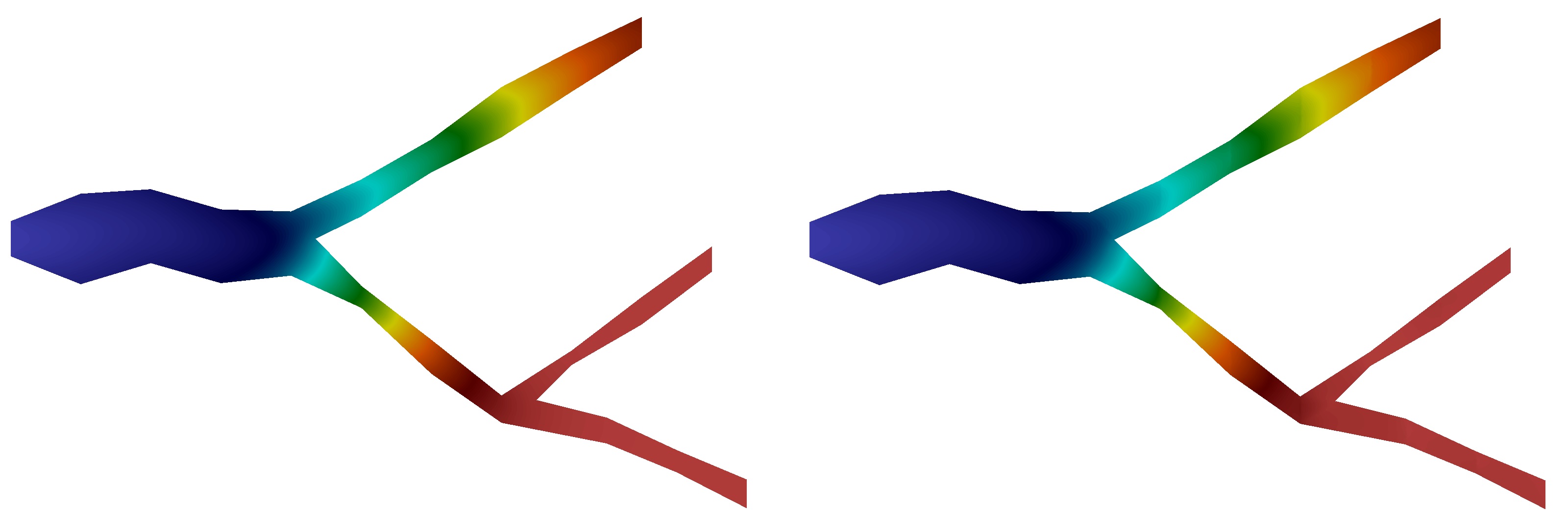
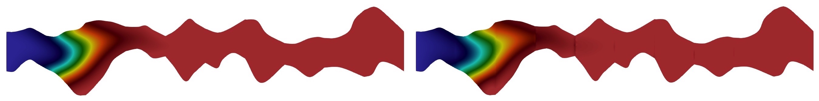
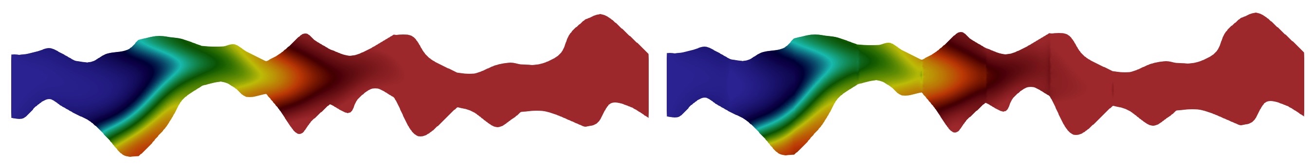
where . In Figures 4 and 5, we depicted the first five multiscale basis functions in and , respectively. Finally, the multiscale space of Type 2 is defined as follows
The Type 1 multiscale space is constructed in a similar way. Instead of flow separation by directions, we define the snapshot space as the collection of the local solutions for flow in all directions
where . To construct a multiscale space, we perform a dimension reduction by the solution of the local spectral problem on snapshot space
| (11) |
with , and
where and are given in (10). We arrange the eigenvalues in increasing order and choose the first eigenvectors corresponding to the first the smallest eigenvalues as the basis functions
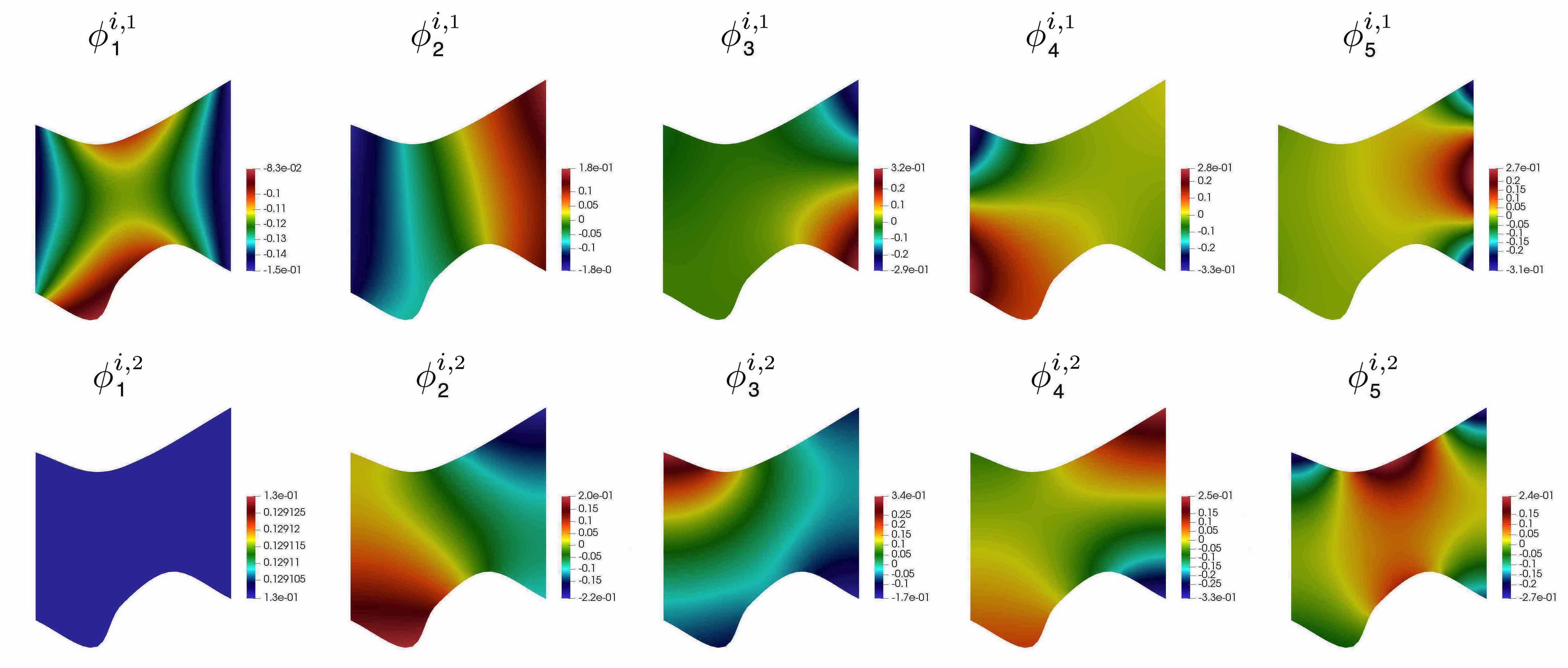
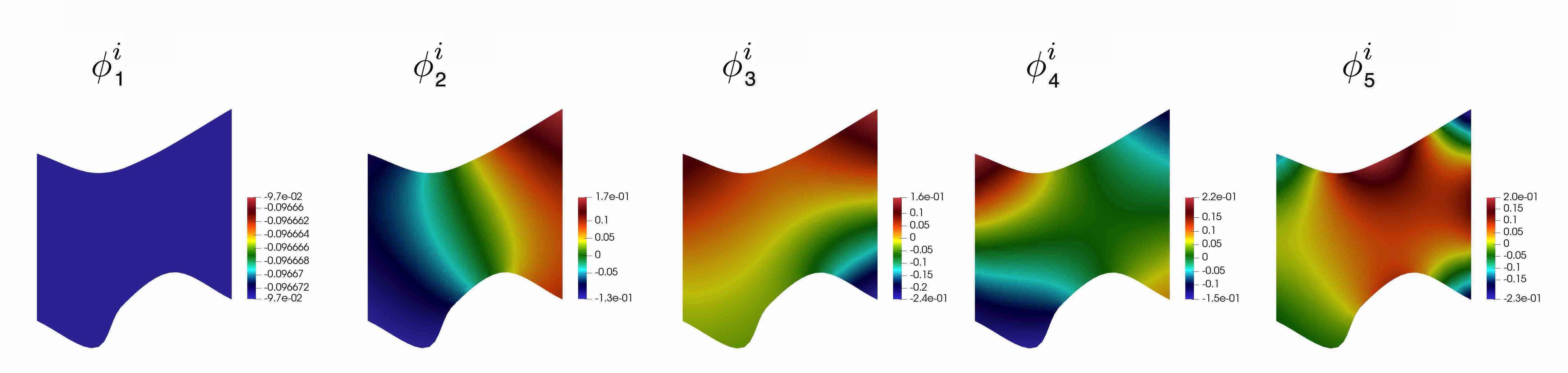
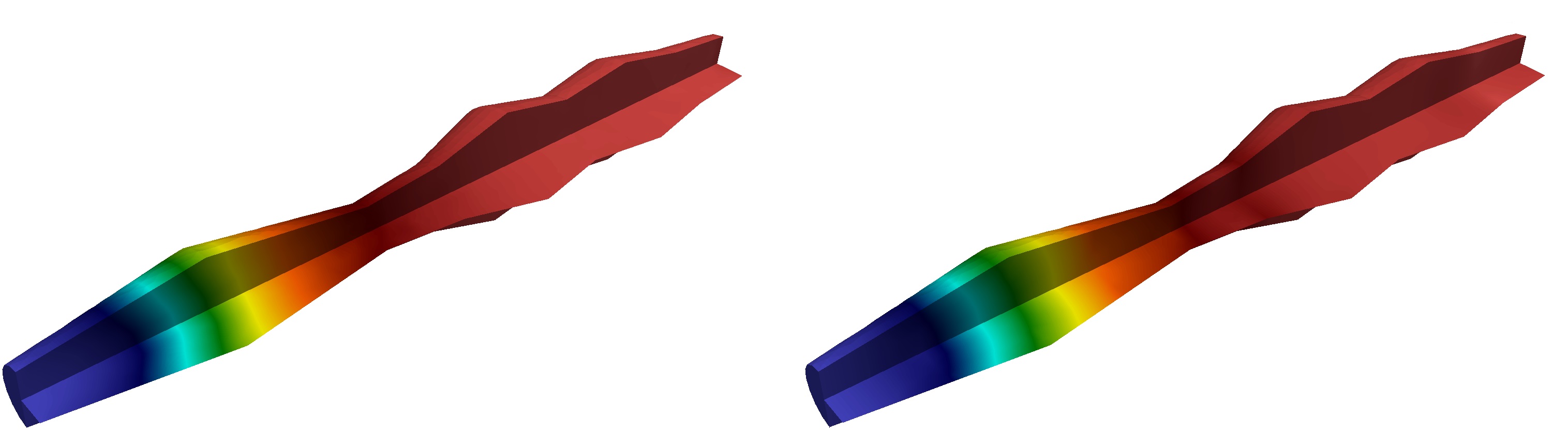
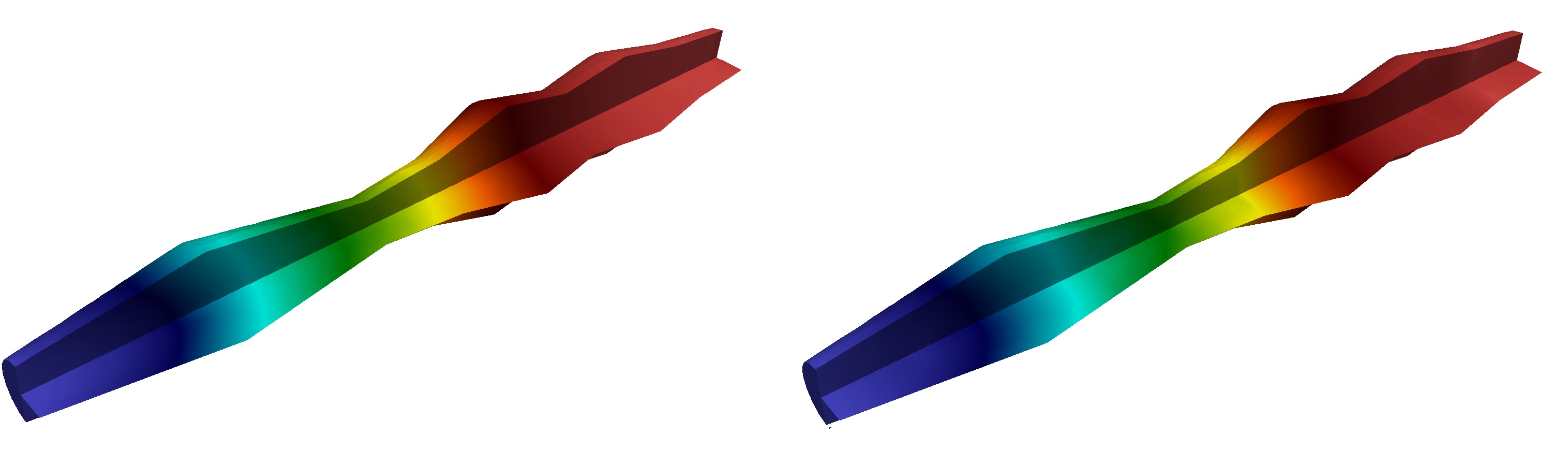
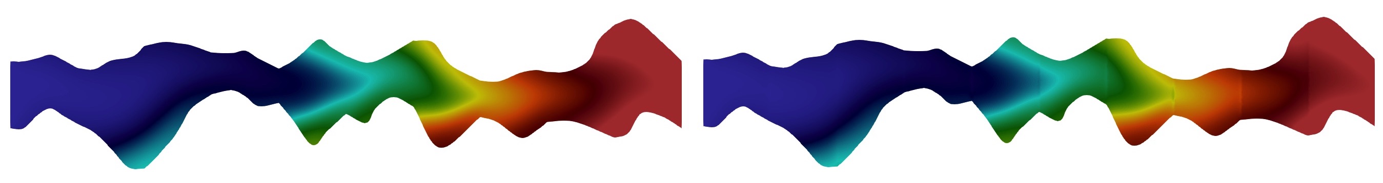
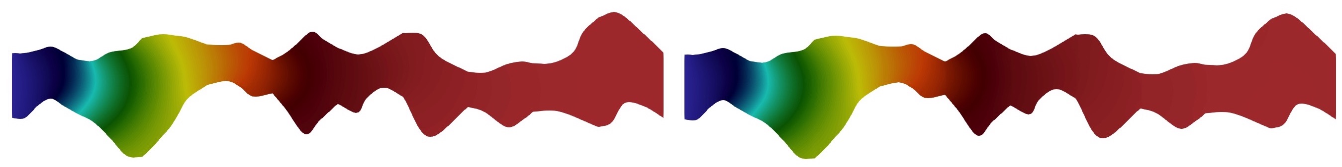
where , . See Figure 6 for an illustration of Type 1 multiscale basis functions.
3.2 Multiscale space for concentration
The construction of the multiscale space for the concentration has a similar concept. The space is constructed for each coarse cell (local domain) for . We consider two types of multiscale spaces:
-
•
Type 1. Multiscale space for transport from all boundaries. Snapshots are constructed for flow in all directions with corresponded spectral problems to dominant mode extraction.
-
•
Type 2. Multiscale space for each boundary transport separately. Snapshot spaces are constructed separately with corresponded spectral problems for each of them.
We will consider two types of boundaries: (1) interface between local domains and (2) reactive wall boundaries . This concept is based on the definition of the coarse grid variables and is similar to the approach that we used in [38, 39].
We will present the construction of the multiscale basis functions for three types of wall boundary conditions for the transport problem
-
•
Dirichlet boundary conditions (DBC):
(12) -
•
Neumann boundary conditions (NBC):
(13) -
•
Robin boundary conditions (RBC):
(14)
We start with the construction of the Type 2 multiscale basis function. The local snapshot space consists of functions which are solutions of the following local problem
| (15) |
where boundary conditions depend on the type of non-homogeneous boundary conditions on wall boundary
-
•
for transport between local domains on interface , we set
and
-
•
for transport from walls boundary
and
Here , where is the number of fine grid facets on the boundary of , and is the discrete delta function defined on and equal to 1 if and zero otherwise. This problem is solved on the fine mesh using an appropriate numerical scheme.
Using these local solutions, we form a local snapshot space for concentration in
and define the snapshot space projection matrix
where .
To reduce the size of the snapshot space, we solve the following local spectral problem in the snapshot space
| (16) |
where
and is the matrix representation of the bilinear form and is the matrix representation of the bilinear form
| (17) |
We remark that the integral in is defined on the boundary of the coarse block and is the fine grid for local domain .
We arrange the eigenvalues in increasing order and choose the first eigenvectors corresponding to the first the smallest eigenvalues as the basis functions
where for and . Finally, the multiscale space of Type 2 is defined as follows
See Figure 7 for an illustration of the multiscale basis functions.
The Type 1 multiscale space is constructed similarly. In the snapshot space, we collect all possible boundary conditions on and solve the following problem
| (18) |
Local solutions are collected as a snapshot space
Dimension reduction of the snapshot space is performed by the solution of the local spectral problem on snapshot space
| (19) |
where , and
where and are given in (17). We arrange the eigenvalues in increasing order and choose the first eigenvectors corresponding to the first the smallest eigenvalues as the basis functions
where for . Multiscale basis functions of Type 1 are presented in Figure 9. We note that, the Type 1 basis functions do not depend on type of boundary conditions on .
Remark 1
For the use of the unsteady convection-diffusion problem instead of the elliptic problem (15) for the construction of the snapshot space, we can use a local problem formulation that is equivalent to the global problem [42, 43]
| (20) |
We will use notations ”Type 1 with time and velocity” and ”Type 2 with time and velocity” in the numerical results section. Illustration of the multiscale basis functions for Type 1 and Type 2 with time and velocity are presented in Figures 10 and 11, respectively.
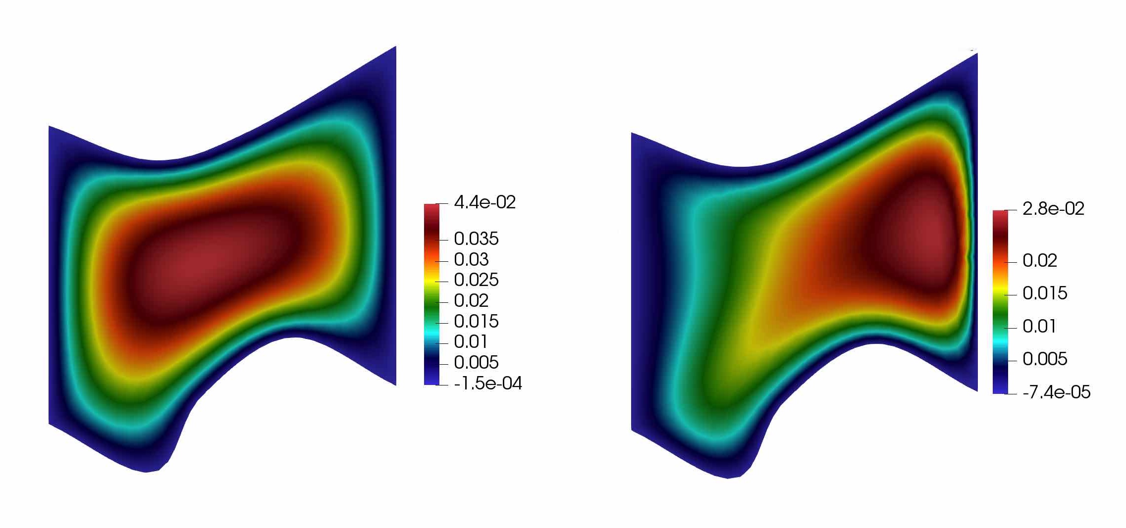
The presented basis functions are associated with the boundary basis functions [44, 45]. In addition to the presented multiscale basis functions, we add one interior basis functions, that is constructed by the solution of the corresponding local problem (15) or (20) with zero Dirichlet boundary conditions on (see Figure 12).
3.3 Coarse scale system
To construct the coarse grid system, we construct projection matrices using the computed multiscale basis functions for velocity and concentration
where we used a single index notation. For Type 1, we have and . For Type 2, we have and . Note that, we use the space of piecewise constant functions for over the coarse grid, and set equal to 1 if and zero otherwise ().
Using these matrices, we have the following computational systems in matrix form:
-
•
Flow problem:
(21) where
and after the solution of the coarse-scale approximation, we reconstruct velocity on a fine grid .
-
•
Transport problem:
(22) where
and reconstruct concentration on the fine grid .
4 Numerical results
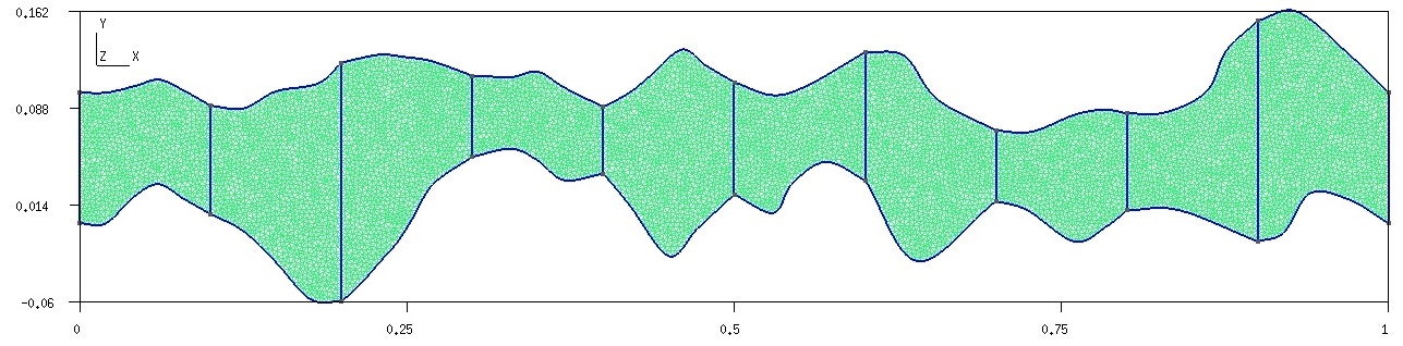
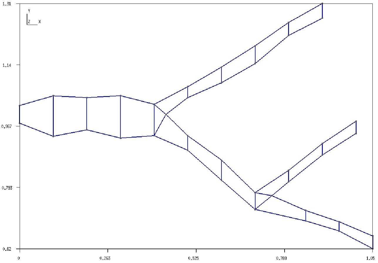
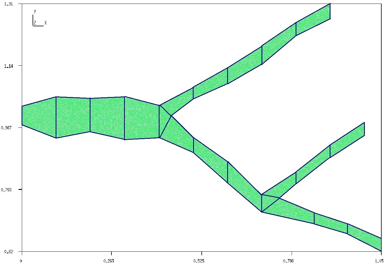
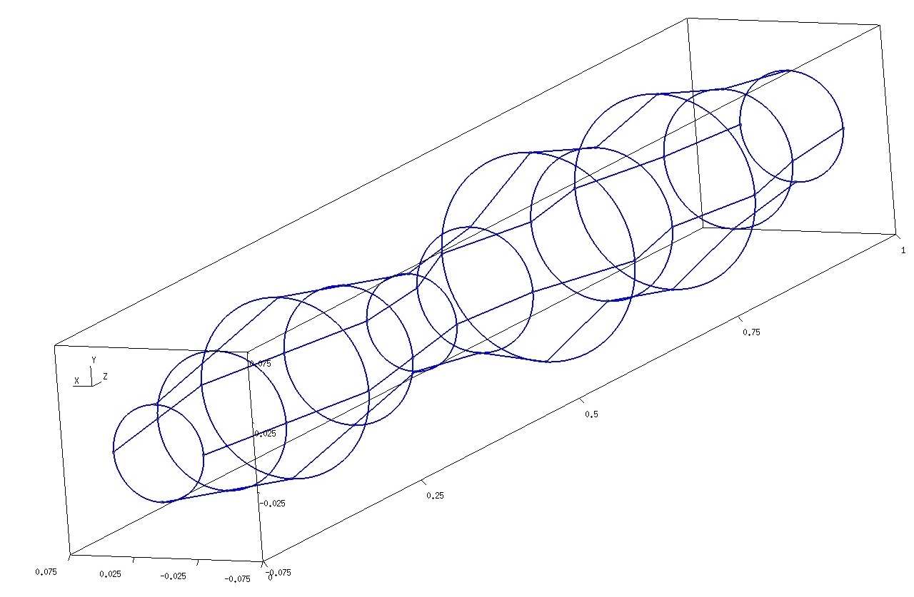
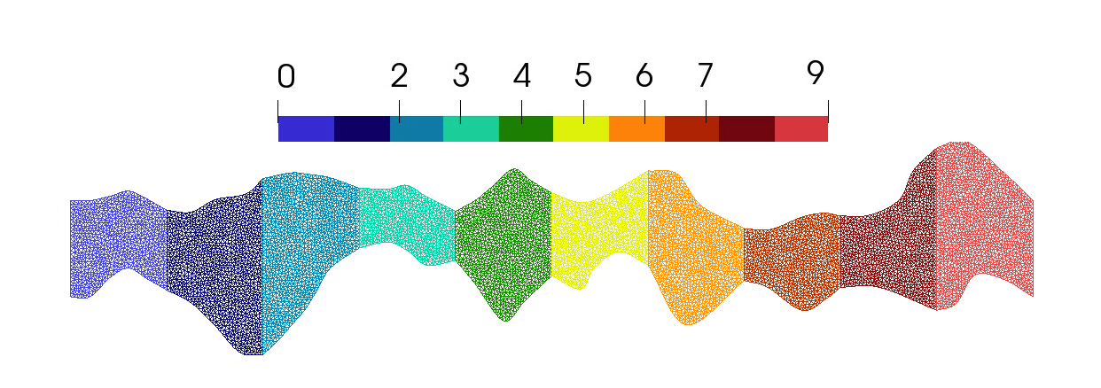
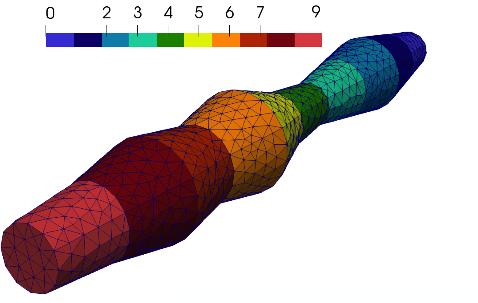
In this section, we will present some numerical results. We will use the following three computational domains (Figure 13) to demonstrate the performance of our method:
-
Geometry 1 with fine grid that contains 17350 cells. Coarse grid contains 10 local domains.
-
Geometry 2 with fine grid that contains 18021 cells. Coarse grid contains 20 local domains.
-
Geometry 3 with fine grid that contains 15094 cells. Coarse grid contains 10 local domains.
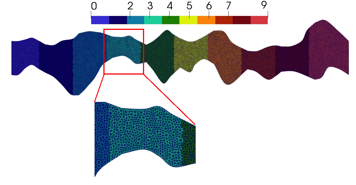
In order to construct structured coarse grids, we explicitly add lines between local domains (coarse grid cells) in geometry construction. For unstructured coarse grid, local domains have a rough interface between local domains. Computational domains with fine and coarse grids are presented in Figure 13 for Geometry 1, 2, and 3. We use Gmsh to construct computational geometries and unstructured fine grids [46]. The numerical implementation is based on the FEniCS library [47].
To investigate the presented multiscale method for solving problems in thin domains with non-homogeneous boundary conditions, we consider the following test:
-
•
Test 1 for different geometries of computational domain. We consider Geometries 1, 2 and 3 (see Figure 13). We consider problems with non-homogeneous Robin boundary conditions for concentration.
-
•
Test 2 for different boundary conditions and diffusion coefficients (, and ). We consider Dirichlet and Neumann non-homogeneous boundary conditions on the wall boundary . In this test, we also investigate different types of multiscale basis functions in detail.
-
•
Test 3 for structured and unstructured coarse grids. We investigate the performance of the multiscale method with a rough interface between local domains (unstructured coarse grid). We also investigate the influence of the multiscale velocity accuracy to the concentration errors.
For flow problem, we set , and . We set for Geometry 1,2 and for Geometry 3 as inflow boundary condition , where with and [48, 3]. Here is the distance to center point and is the radius of left boundary , where , for Geometry 1, , for Geometry 2, and , for Geometry 3.
We calculate relative errors in norm in percentage
where and are multiscale solutions, and are reference solutions.
4.1 Test 1 (different geometries)
We consider a test problem with non-homogeneous Robin boundary condition for concentration
where , and . As initial conditions, we set and . For the inflow (left) boundary, we set for . We perform simulations for (Geometry 1), (Geometry 2) and (Geometry 3) with 40 time iterations. The coarse grid is structured with 20 local domains for Geometry 2, and with 10 local domains for Geometry 1 and 3. In Figure 14, we show local domain markers.
| Type 1 | |
|---|---|
| (%) | |
| Geometry 1 | |
| 110 (10) | 11.70 |
| 210 (20) | 6.013 |
| 410 (40) | 1.536 |
| 610 (60) | 1.086 |
| 810 (80) | 1.064 |
| Geometry 2 | |
| 220 (10) | 27.20 |
| 420 (20) | 6.205 |
| 820 (40) | 1.485 |
| 1220 (60) | 1.369 |
| 1620 (80) | 1.374 |
| Geometry 3 | |
| 160 (15) | 36.70 |
| 310 (30) | 10.76 |
| 610 (60) | 9.493 |
| 910 (90) | 8.548 |
| 1210 (120) | 5.657 |
| Type 2 | |
|---|---|
| (%) | |
| Geometry 1 | |
| 110 (5) | 19.85 |
| 210 (10) | 10.52 |
| 410 (20) | 3.230 |
| 610 (30) | 1.756 |
| 810 (40) | 1.346 |
| Geometry 2 | |
| 220 (5) | 31.51 |
| 420 (10) | 10.08 |
| 820 (20) | 3.570 |
| 1220 (30) | 1.906 |
| 1620 (40) | 1.521 |
| Geometry 3 | |
| 160 (5) | 15.96 |
| 310 (10) | 10.63 |
| 610 (20) | 6.548 |
| 910 (30) | 4.167 |
| 1210 (40) | 4.082 |
| Type 1, without velocity | ||||
| ) | ) | ) | ) | |
| Geometry 1 | ||||
| 30 (2) | 42.27 | 38.93 | 37.68 | 37.64 |
| 70 (6) | 6.747 | 7.675 | 8.587 | 9.206 |
| 110 (10) | 3.160 | 3.818 | 4.269 | 4.549 |
| 210 (20) | 1.954 | 2.228 | 2.294 | 2.300 |
| 410 (40) | 1.924 | 2.189 | 2.252 | 2.259 |
| 610 (60) | 1.920 | 2.184 | 2.247 | 2.253 |
| 810 (80) | 1.916 | 2.177 | 2.236 | 2.240 |
| Geometry 2 | ||||
| 60 (2) | 60.30 | 61.20 | 55.67 | 46.25 |
| 140 (6) | 1.931 | 2.021 | 2.668 | 2.766 |
| 220 (10) | 1.784 | 1.495 | 1.471 | 1.451 |
| 420 (20) | 1.041 | 1.074 | 1.059 | 0.989 |
| 820 (40) | 1.048 | 1.315 | 1.069 | 0.997 |
| 1220 (60) | 1.054 | 1.085 | 1.075 | 1.004 |
| 1620 (80) | 1.058 | 1.088 | 1.079 | 1.009 |
| Geometry 3 | ||||
| 30 (2) | 16.17 | 16.07 | 21.69 | 23.32 |
| 70 (6) | 16.60 | 14.86 | 15.52 | 15.85 |
| 110 (10) | 16.23 | 14.50 | 15.15 | 15.47 |
| 210 (20) | 5.274 | 4.940 | 5.252 | 5.648 |
| 410 (40) | 4.871 | 4.607 | 4.947 | 5.338 |
| 610 (60) | 4.623 | 4.391 | 4.715 | 5.094 |
| 810 (80) | 4.568 | 4.337 | 4.659 | 5.037 |
| Type 2, without velocity | ||||
| ) | ) | ) | ) | |
| Geometry 1 | ||||
| 30 (1) | 46.99 | 53.03 | 52.54 | 50.25 |
| 70 (3) | 4.111 | 4.070 | 4.746 | 5.154 |
| 110 (5) | 2.653 | 2.851 | 2.973 | 2.989 |
| 210 (10) | 1.950 | 2.196 | 2.236 | 2.224 |
| 410 (20) | 1.906 | 2.127 | 2.154 | 2.140 |
| 610 (30) | 1.902 | 2.121 | 2.148 | 2.135 |
| 810 (40) | 1.901 | 2.120 | 2.147 | 2.134 |
| Geometry 2 | ||||
| 60 (1) | 73.44 | 84.91 | 87.34 | 87.06 |
| 140 (3) | 2.256 | 2.205 | 2.349 | 2.249 |
| 220 (5) | 1.341 | 1.569 | 1.692 | 1.581 |
| 420 (10) | 1.142 | 1.204 | 1.228 | 1.144 |
| 820 (20) | 1.145 | 1.190 | 1.215 | 1.144 |
| 1220 (30) | 1.148 | 1.191 | 1.218 | 1.149 |
| 1620 (40) | 1.149 | 1.191 | 1.219 | 1.150 |
| Geometry 3 | ||||
| 30 (1) | 58.70 | 71.74 | 74.82 | 73.37 |
| 70 (3) | 2.322 | 1.866 | 2.071 | 2.229 |
| 110 (5) | 2.306 | 1.895 | 2.051 | 2.214 |
| 210 (10) | 2.317 | 2.142 | 2.348 | 2.586 |
| 410 (20) | 1.892 | 1.773 | 1.992 | 2.210 |
| 610 (30) | 1.691 | 1.595 | 1.792 | 1.988 |
| 810 (40) | 1.651 | 1.552 | 1.746 | 1.938 |
| Type 1, with velocity | ||||
| ) | ) | ) | ) | |
| Geometry 1 | ||||
| 30 (2) | 60.48 | 66.48 | 65.71 | 63.81 |
| 70 (6) | 41.95 | 45.45 | 43.60 | 40.94 |
| 110 (10) | 31.93 | 34.33 | 31.66 | 28.18 |
| 210 (20) | 6.114 | 7.652 | 6.285 | 4.931 |
| 410 (40) | 1.747 | 1.776 | 1.572 | 1.376 |
| 610 (60) | 1.742 | 1.762 | 1.555 | 1.359 |
| 810 (80) | 1.741 | 1.758 | 1.549 | 1.352 |
| Geometry 2 | ||||
| 60 (2) | 65.49 | 64.93 | 58.22 | 48.53 |
| 140 (6) | 47.06 | 53.16 | 53.16 | 42.65 |
| 220 (10) | 16.22 | 15.71 | 15.73 | 14.42 |
| 420 (20) | 1.467 | 1.491 | 1.474 | 1.275 |
| 820 (40) | 1.277 | 1.315 | 1.274 | 1.089 |
| 1220 (60) | 1.262 | 1.302 | 1.259 | 1.075 |
| 1620 (80) | 1.252 | 1.293 | 1.248 | 1.065 |
| Geometry 3 | ||||
| 30 (2) | 43.35 | 39.21 | 40.01 | 40.01 |
| 70 (6) | 22.71 | 21.47 | 21.47 | 21.47 |
| 110 (10) | 21.90 | 20.70 | 21.68 | 20.55 |
| 210 (20) | 15.56 | 14.70 | 15.34 | 15.34 |
| 410 (40) | 12.48 | 12.05 | 12.96 | 13.77 |
| 610 (60) | 11.50 | 11.24 | 12.14 | 12.94 |
| 810 (80) | 11.20 | 10.98 | 11.88 | 12.68 |
| Type 2, with velocity | ||||
| ) | ) | ) | ) | |
| Geometry 1 | ||||
| 30 (1) | 49.91 | 53.68 | 52.64 | 50.36 |
| 70 (3) | 26.22 | 24.27 | 21.11 | 19.47 |
| 110 (5) | 14.63 | 13.24 | 9.694 | 7.351 |
| 210 (10) | 6.909 | 5.760 | 3.943 | 2.372 |
| 410 (20) | 1.867 | 2.004 | 1.870 | 1.701 |
| 610 (30) | 1.850 | 1.979 | 1.842 | 1.674 |
| 810 (40) | 1.846 | 1.973 | 1.836 | 1.669 |
| Geometry 2 | ||||
| 60 (1) | 48.37 | 53.67 | 52.88 | 49.64 |
| 140 (3) | 14.56 | 19.78 | 20.14 | 15.63 |
| 220 (5) | 12.46 | 16.05 | 16.30 | 12.98 |
| 420 (10) | 1.474 | 1.517 | 1.532 | 1.350 |
| 820 (20) | 1.308 | 1.362 | 1.340 | 1.159 |
| 1220 (30) | 1.282 | 1.338 | 1.310 | 1.133 |
| 1620 (40) | 1.272 | 1.331 | 1.302 | 1.126 |
| Geometry 3 | ||||
| 30 (1) | 32.10 | 32.21 | 34.24 | 32.98 |
| 70 (3) | 32.09 | 32.19 | 34.22 | 32.96 |
| 110 (5) | 10.03 | 9.976 | 10.90 | 11.25 |
| 210 (10) | 7.491 | 7.609 | 8.511 | 8.736 |
| 410 (20) | 6.934 | 7.026 | 7.702 | 8.124 |
| 610 (30) | 6.189 | 6.384 | 7.065 | 7.484 |
| 810 (40) | 6.028 | 6.234 | 6.909 | 7.320 |
We consider the performance of the presented method for the solution of transport and flow problems in different computational domains. We consider two types of multiscale basis functions (see Section 3). and are the number of the multiscale basis functions for concentration and velocity, respectively. and are the number of degrees of freedom for reference (fine grid) solution. and are the numbers of degrees of freedom for a multiscale solution. The reference solution is performed on the fine grid using IPDG approximation presented in Section 2. We used linear basis functions for both velocity and concentration fields on the fine grid. Therefore, and . For multiscale solver, we have , for Type 1 and , for Type 2 multiscale basis functions.
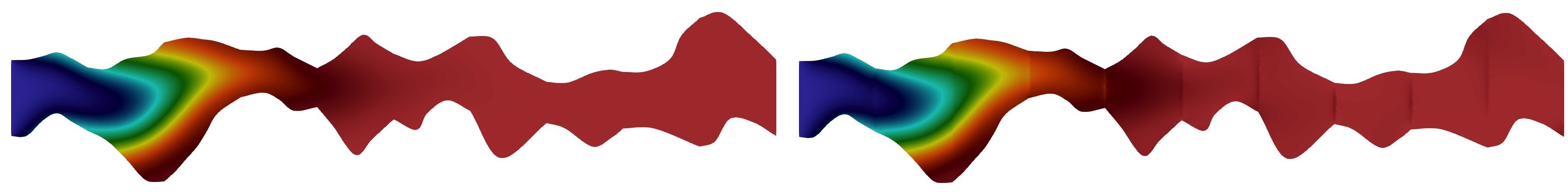
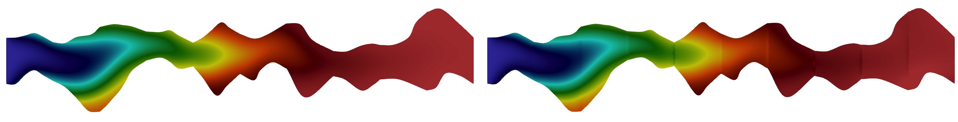
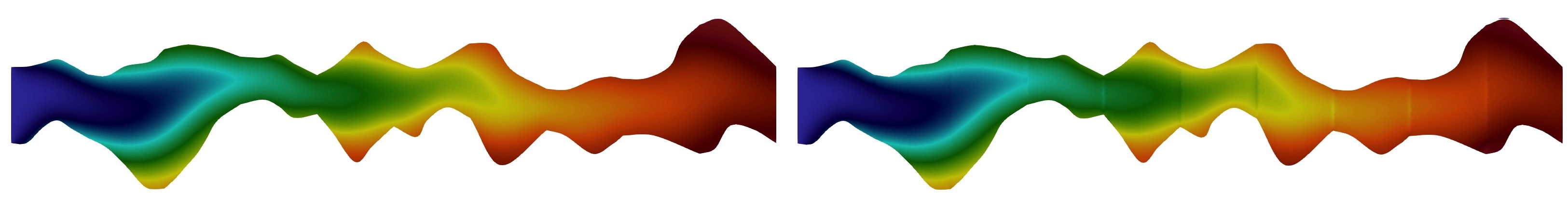
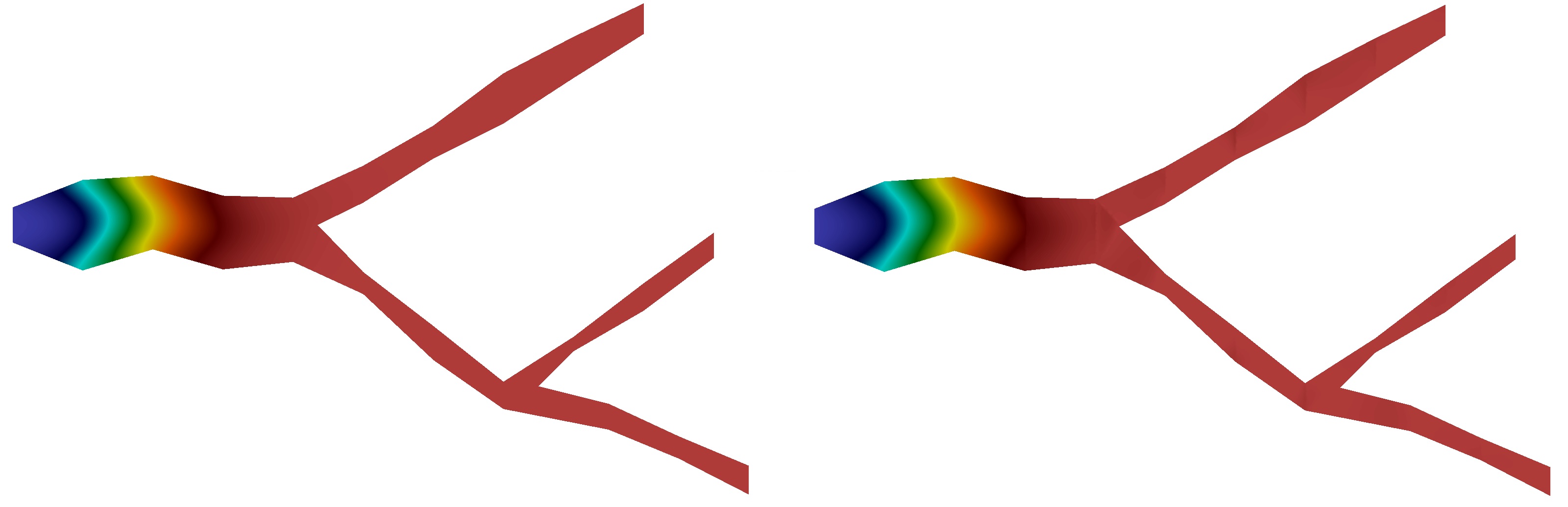
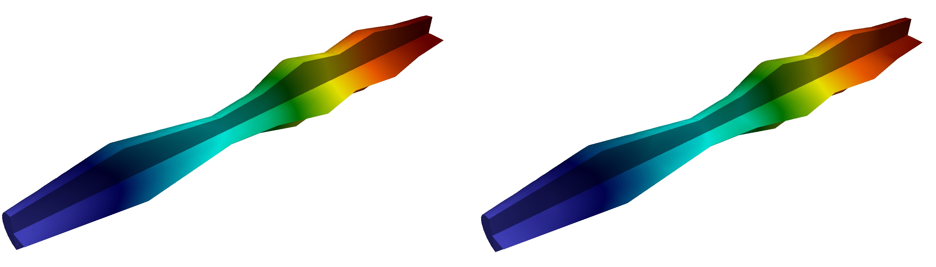
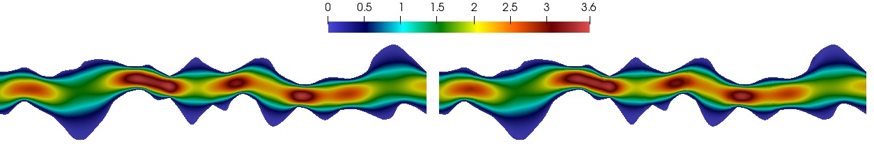
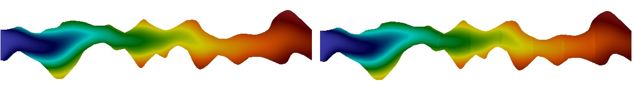
Because velocity does not depend on the concentration in our test problems. We start with results for flow problems. In Figure 15, we present reference and multiscale solutions for Geometries 1, 2, and 3. We depicted the magnitude of the velocity field at the final time. In a multiscale solver, we used multiscale basis functions for each direction (Type 2). For Geometry 1, we have and (0.33 % from ). For Geometry 2, we have and (0.65 % from ). For Geometry 3, we have and (0.31 % from ). We observe a good accuracy of the presented method with huge reduction of the discrete system size.
In Table 1, we present relative errors in % for velocity between reference solution and multiscale solution with different numbers of the multiscale basis functions at the final times. We observe a reduction of the error with an increasing number of multiscale basis functions for all geometries. For example for 40 multiscale basis functions of Type 2, we have % of error for Geometry 1, % of error for Geometry 2, and % of error for Geometry 3. For Type 1 and 2, we observe similar errors for two-dimensional problems (Geometry 1 and 2). For three - dimensional domain in Geometry 3, we obtain better results with Type 2 multiscale basis functions.
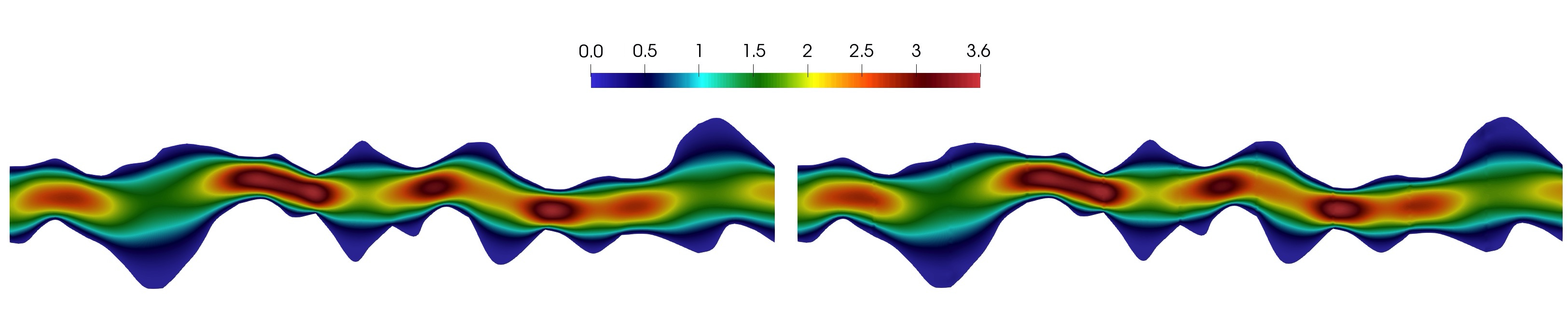
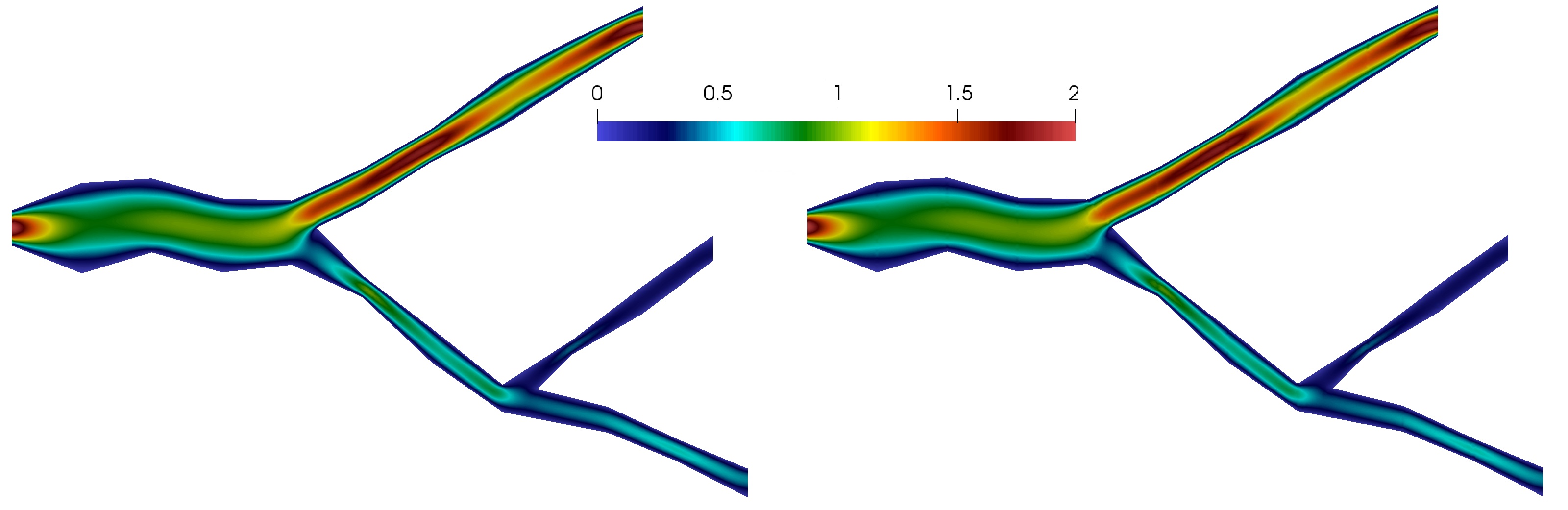
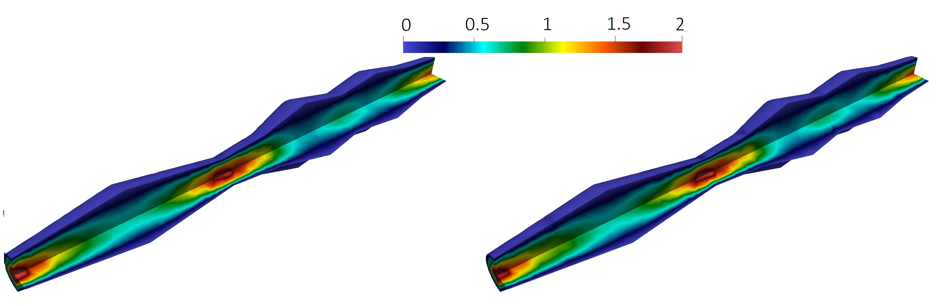
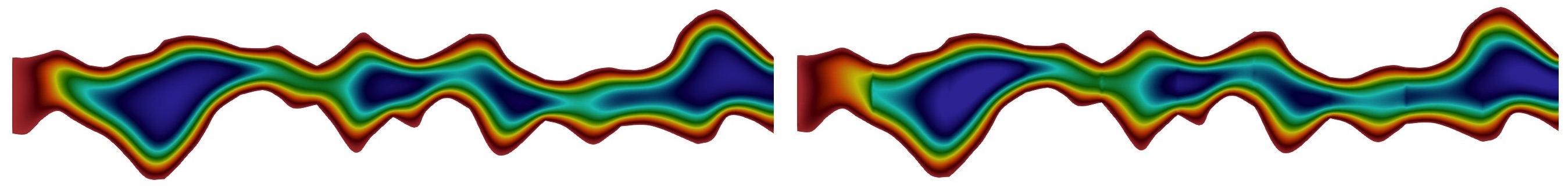
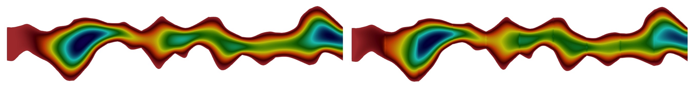
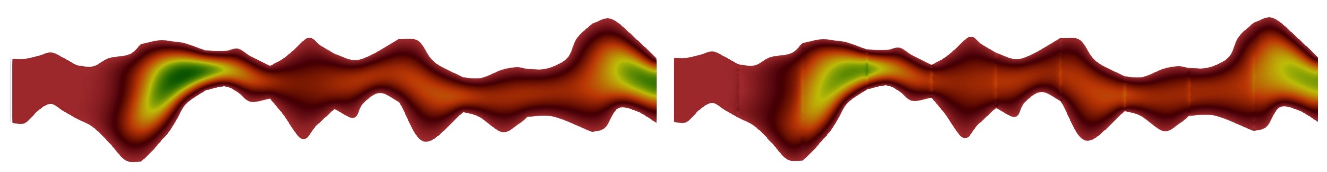
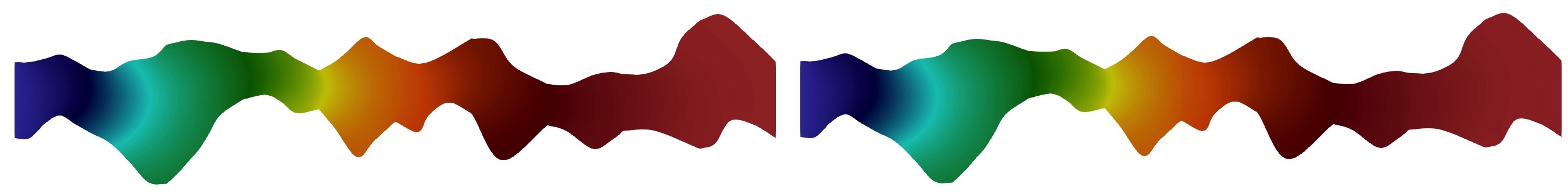
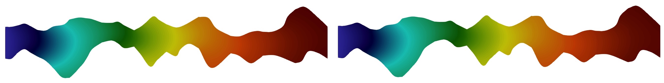
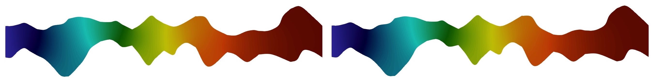
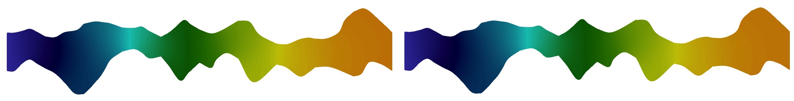
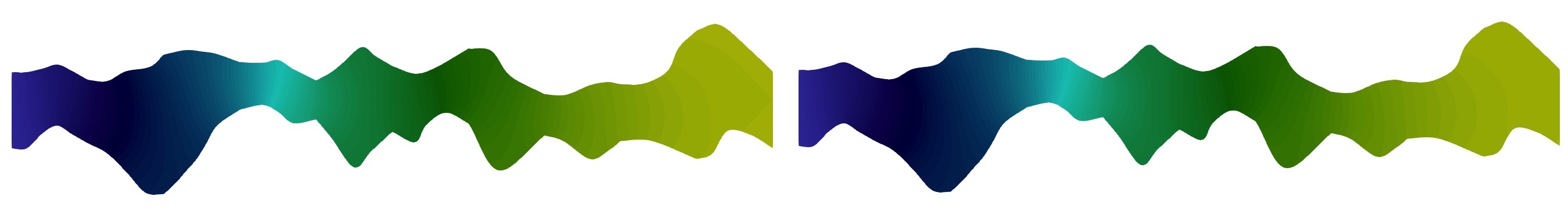
In Figures 16, 17 and 18, we present concentration distributions for the reference (fine scale) and multiscale solutions at different time layers for and . In these calculations, we used a fixed number of multiscale basis functions for the velocity field ( of Type 2). We will investigate the influence of the velocity accuracy on the concentration solution later in Test 3. In figures, we presented results for multiscale basis functions for each type of local domain boundaries (Type 2). For Geometry 1 (Figure 16), we have and (0.78 % from ). For Geometry 2 Figure 17), we have and (1.5 % from ). For Geometry 3 Figure 18), we have and (0.67 % from ). We observe good results of the presented method for solving transport problems for all three geometries.
We present numerical results in Tables 2 and 3 for different number of multiscale basis functions for concentration (Type 1 and 2) for a fixed number of multiscale basis functions for velocity field ( of Type 2). Relative errors for concentrations are presented for four time layers with and . We can obtain good multiscale solution when we take a sufficient number of multiscale basis functions for pressure and for displacements. For example, we obtain near 40 % of concentration error, when we take 3 multiscale basis functions of Type 1 and near 20 % for Type 2. For 40 multiscale basis functions of Type 2, the error reduce to % for Geometry 1, % for Geometry 2, and % for Geometry 3. For two-dimensional problems (Geometry 1 and 2), we obtain a similar error for Type 1 and 2 multiscale basis functions. However, for three - dimensional problem (Geometry 3), the multiscale basis of Type 2 is better.
We observe that the presented multiscale method provides good results with small errors and huge reduction of the system size for all three test geometries. For the presented test problem in the 3D case is better to use basis functions without information on the velocity field. For the 2D result, we observe similar errors for basis with and without velocity. For three-dimensional problem Type 2 multiscale basis functions are better than Type 1 due to direct definitions of the flow and transport directions. However, for 2D problem, we obtain similar results for Type 1 and 2 basis functions.
4.2 Test 2 (different boundary conditions and diffusion coefficients)
Next, we consider the efficiency of the presented method for the solution of the transport problem with different types of boundary conditions and different values of diffusion coefficient .
| with velocity | ||||
| ) | ) | ) | ) | |
| Type 1, without time | ||||
| 30 (2) | 51.74 | 36.78 | 26.43 | 18.88 |
| 70 (6) | 51.75 | 36.82 | 26.45 | 18.90 |
| 110 (10) | 44.35 | 31.52 | 22.54 | 16.19 |
| 210 (20) | 18.04 | 11.93 | 8.893 | 6.877 |
| 410 (40) | 9.781 | 5.784 | 4.241 | 3.229 |
| 610 (60) | 9.205 | 5.434 | 3.993 | 3.036 |
| 810 (80) | 9.114 | 5.366 | 3.946 | 3.001 |
| Type 2, without time | ||||
| 30 (1) | 44.40 | 31.76 | 23.15 | 16.78 |
| 70 (3) | 17.92 | 11.85 | 8.891 | 6.782 |
| 110 (5) | 12.42 | 6.768 | 4.681 | 3.486 |
| 210 (10) | 9.150 | 5.210 | 3.815 | 2.906 |
| 410 (20) | 8.845 | 5.065 | 3.848 | 2.888 |
| 610 (30) | 8.831 | 5.132 | 3.787 | 2.887 |
| 810 (40) | 8.829 | 5.131 | 3.786 | 2.886 |
| Type 2, with time | ||||
| 30 (1) | 44.40 | 31.76 | 23.15 | 16.78 |
| 70 (3) | 17.92 | 11.86 | 8.892 | 6.783 |
| 110 (5) | 12.42 | 6.768 | 4.681 | 3.487 |
| 210 (10) | 9.150 | 5.210 | 3.815 | 2.906 |
| 410 (20) | 8.844 | 5.135 | 3.788 | 2.888 |
| 610 (30) | 8.831 | 5.132 | 3.787 | 2.887 |
| 810 (40) | 8.829 | 5.131 | 3.786 | 2.886 |
| without velocity | ||||
| ) | ) | ) | ) | |
| Type 1, with time | ||||
| 30 (2) | 67.69 | 49.62 | 34.35 | 23.66 |
| 70 (6) | 67.83 | 49.75 | 34.47 | 23.78 |
| 110 (10) | 64.16 | 48.15 | 33.99 | 23.80 |
| 210 (20) | 15.70 | 13.12 | 11.58 | 9.439 |
| 410 (40) | 9.781 | 5.065 | 3.848 | 2.939 |
| 610 (60) | 6.883 | 4.778 | 3.650 | 2.779 |
| 810 (80) | 6.831 | 4.736 | 3.619 | 2.754 |
| Type 2, without time | ||||
| 30 (1) | 89.85 | 83.50 | 73.50 | 65.06 |
| 70 (3) | 62.18 | 62.39 | 59.84 | 56.96 |
| 110 (5) | 51.05 | 48.08 | 42.41 | 36.61 |
| 210 (10) | 7.397 | 4.893 | 3.972 | 3.309 |
| 410 (20) | 6.750 | 4.405 | 3.397 | 2.656 |
| 610 (30) | 6.728 | 4.392 | 3.381 | 2.648 |
| 810 (40) | 6.726 | 4.392 | 3.381 | 2.649 |
| Type 2, with time | ||||
| 30 (1) | 89.85 | 83.51 | 73.50 | 65.07 |
| 70 (3) | 62.18 | 62.40 | 59.85 | 56.97 |
| 110 (5) | 51.03 | 48.06 | 42.40 | 36.60 |
| 210 (10) | 7.397 | 4.892 | 3.971 | 3.308 |
| 410 (20) | 6.750 | 4.405 | 3.398 | 2.656 |
| 610 (30) | 6.728 | 4.392 | 3.381 | 2.648 |
| 810 (40) | 6.726 | 4.393 | 3.381 | 2.649 |
| without velocity | ||||
| ) | ) | ) | ) | |
| Type 1, without time | ||||
| 30 (2) | 45.87 | 48.36 | 50.73 | 48.27 |
| 70 (6) | 5.842 | 6.302 | 7.917 | 11.05 |
| 110 (10) | 2.860 | 3.474 | 4.482 | 6.459 |
| 210 (20) | 2.131 | 2.703 | 3.338 | 4.570 |
| 410 (40) | 2.104 | 2.670 | 3.284 | 4.465 |
| 610 (60) | 2.102 | 2.667 | 3.279 | 4.453 |
| 810 (80) | 2.099 | 2.664 | 3.274 | 4.442 |
| Type 2, without time | ||||
| 30 (1) | 75.71 | 89.67 | 93.60 | 93.30 |
| 70 (3) | 6.233 | 6.465 | 8.005 | 11.93 |
| 110 (5) | 4.621 | 6.042 | 7.537 | 10.75 |
| 210 (10) | 3.385 | 4.431 | 5.718 | 8.192 |
| 410 (20) | 3.164 | 4.037 | 5.214 | 7.593 |
| 610 (30) | 3.088 | 3.928 | 5.065 | 7.375 |
| 810 (40) | 3.056 | 3.896 | 5.021 | 7.301 |
| Type 2, with time | ||||
| 30 (1) | 67.10 | 82.64 | 88.56 | 88.73 |
| 70 (3) | 4.373 | 4.409 | 5.511 | 8.065 |
| 110 (5) | 2.680 | 3.212 | 4.097 | 5.803 |
| 210 (10) | 2.143 | 2.723 | 3.338 | 4.492 |
| 410 (20) | 2.123 | 2.691 | 3.290 | 4.409 |
| 610 (30) | 2.121 | 2.689 | 3.287 | 4.405 |
| 810 (40) | 2.120 | 2.688 | 3.286 | 4.402 |
| with velocity | ||||
| ) | ) | ) | ) | |
| Type 1, with time | ||||
| 30 (2) | 69.34 | 84.22 | 89.44 | 89.28 |
| 70 (6) | 49.09 | 61.96 | 67.20 | 64.77 |
| 110 (10) | 36.89 | 47.61 | 51.47 | 46.71 |
| 210 (20) | 7.022 | 11.53 | 13.35 | 16.50 |
| 410 (40) | 2.080 | 2.587 | 2.744 | 2.371 |
| 610 (60) | 2.071 | 2.565 | 2.713 | 2.336 |
| 810 (80) | 2.069 | 2.559 | 2.705 | 2.327 |
| Type 2, without time | ||||
| 30 (1) | 47.37 | 56.09 | 61.62 | 59.57 |
| 70 (3) | 28.27 | 31.79 | 31.76 | 24.81 |
| 110 (5) | 15.85 | 18.89 | 18.45 | 15.28 |
| 210 (10) | 8.635 | 8.903 | 7.371 | 9.659 |
| 410 (20) | 2.126 | 2.669 | 2.823 | 2.283 |
| 610 (30) | 2.112 | 2.651 | 2.801 | 2.272 |
| 810 (40) | 2.109 | 2.646 | 2.797 | 2.270 |
| Type 2, with time | ||||
| 30 (1) | 47.38 | 56.10 | 61.64 | 59.59 |
| 70 (3) | 28.26 | 31.78 | 31.76 | 24.80 |
| 110 (5) | 15.85 | 18.89 | 18.45 | 15.29 |
| 210 (10) | 8.636 | 8.902 | 7.368 | 9.661 |
| 410 (20) | 2.126 | 2.669 | 2.822 | 2.283 |
| 610 (30) | 2.112 | 2.651 | 2.801 | 2.272 |
| 810 (40) | 2.109 | 2.646 | 2.797 | 2.270 |
| without velocity | ||||
| ) | ) | ) | ) | |
| Type 1, without time | ||||
| 30 (2) | 45.03 | 46.24 | 45.64 | 44.56 |
| 70 (6) | 3.870 | 3.959 | 3.910 | 3.813 |
| 110 (10) | 0.843 | 0.842 | 0.841 | 0.816 |
| 210 (20) | 0.505 | 0.502 | 0.505 | 0.492 |
| 410 (40) | 0.471 | 0.465 | 0.470 | 0.462 |
| 610 (60) | 0.469 | 0.462 | 0.468 | 0.460 |
| 810 (80) | 0.468 | 0.462 | 0.467 | 0.459 |
| Type 2, without time | ||||
| 30 (1) | 93.96 | 93.31 | 92.55 | 92.02 |
| 70 (3) | 3.892 | 3.337 | 2.978 | 2.793 |
| 110 (5) | 0.486 | 0.488 | 0.503 | 0.509 |
| 210 (10) | 0.384 | 0.361 | 0.362 | 0.362 |
| 410 (20) | 0.380 | 0.357 | 0.356 | 0.357 |
| 610 (30) | 0.380 | 0.356 | 0.355 | 0.356 |
| 810 (40) | 0.380 | 0.356 | 0.356 | 0.356 |
| Type 2, with time | ||||
| 30 (1) | 93.96 | 93.31 | 92.55 | 92.02 |
| 70 (3) | 3.893 | 3.339 | 2.980 | 2.795 |
| 110 (5) | 0.486 | 0.488 | 0.503 | 0.509 |
| 210 (10) | 0.384 | 0.361 | 0.362 | 0.363 |
| 410 (20) | 0.380 | 0.357 | 0.356 | 0.357 |
| 610 (30) | 0.380 | 0.356 | 0.355 | 0.356 |
| 810 (40) | 0.380 | 0.356 | 0.355 | 0.356 |
| with velocity | ||||
| ) | ) | ) | ) | |
| Type 1, with time | ||||
| 30 (2) | 48.32 | 51.01 | 50.58 | 49.42 |
| 70 (6) | 6.069 | 6.268 | 6.097 | 5.845 |
| 110 (10) | 0.827 | 0.875 | 0.870 | 0.826 |
| 210 (20) | 0.516 | 0.569 | 0.570 | 0.537 |
| 410 (40) | 0.475 | 0.524 | 0.528 | 0.502 |
| 610 (60) | 0.472 | 0.521 | 0.525 | 0.499 |
| 810 (80) | 0.472 | 0.520 | 0.524 | 0.498 |
| Type 2, without time | ||||
| 30 (1) | 71.43 | 75.52 | 73.94 | 72.40 |
| 70 (3) | 8.661 | 8.862 | 8.827 | 8.631 |
| 110 (5) | 1.208 | 1.440 | 1.440 | 1.492 |
| 210 (10) | 0.509 | 0.619 | 0.656 | 0.648 |
| 410 (20) | 0.408 | 0.467 | 0.490 | 0.486 |
| 610 (30) | 0.400 | 0.454 | 0.475 | 0.472 |
| 810 (40) | 0.399 | 0.451 | 0.472 | 0.469 |
| Type 2, with time | ||||
| 30 (1) | 71.43 | 75.52 | 73.94 | 72.40 |
| 70 (3) | 8.662 | 8.863 | 8.828 | 8.632 |
| 110 (5) | 1.209 | 1.441 | 1.514 | 1.493 |
| 210 (10) | 0.509 | 0.619 | 0.656 | 0.649 |
| 410 (20) | 0.408 | 0.467 | 0.490 | 0.487 |
| 610 (30) | 0.400 | 0.454 | 0.475 | 0.472 |
| 810 (40) | 0.399 | 0.452 | 0.472 | 0.469 |
| without velocity | ||||
| ) | ) | ) | ) | |
| Type 1, without time | ||||
| 30 (2) | 82.00 | 80.87 | 78.91 | 78.04 |
| 70 (6) | 9.095 | 10.93 | 11.00 | 10.74 |
| 110 (10) | 2.086 | 2.625 | 2.636 | 2.562 |
| 210 (20) | 1.344 | 1.707 | 1.718 | 1.671 |
| 410 (40) | 1.149 | 1.458 | 1.468 | 1.428 |
| 610 (60) | 1.128 | 1.431 | 1.442 | 1.402 |
| 810 (80) | 1.120 | 1.421 | 1.431 | 1.392 |
| Type 2, without time | ||||
| 30 (1) | 98.76 | 98.43 | 98.25 | 98.17 |
| 70 (3) | 7.119 | 7.728 | 7.684 | 7.536 |
| 110 (5) | 0.699 | 0.872 | 0.870 | 0.846 |
| 210 (10) | 0.197 | 0.251 | 0.253 | 0.246 |
| 410 (20) | 0.114 | 0.143 | 0.145 | 0.141 |
| 610 (30) | 0.109 | 0.136 | 0.138 | 0.134 |
| 810 (40) | 0.108 | 0.135 | 0.137 | 0.133 |
| Type 2, with time | ||||
| 30 (1) | 98.76 | 98.43 | 98.25 | 98.17 |
| 70 (3) | 7.119 | 7.728 | 7.684 | 7.536 |
| 110 (5) | 0.699 | 0.872 | 0.872 | 0.846 |
| 210 (10) | 0.197 | 0.251 | 0.251 | 0.246 |
| 410 (20) | 0.114 | 0.143 | 0.145 | 0.141 |
| 610 (30) | 0.109 | 0.136 | 0.138 | 0.134 |
| 810 (40) | 0.108 | 0.135 | 0.137 | 0.133 |
| with velocity | ||||
| ) | ) | ) | ) | |
| Type 1, with time | ||||
| 30 (2) | 82.06 | 80.92 | 78.95 | 78.09 |
| 70 (6) | 9.142 | 10.99 | 11.05 | 10.79 |
| 110 (10) | 2.094 | 2.636 | 2.647 | 2.572 |
| 210 (20) | 1.354 | 1.720 | 1.731 | 1.683 |
| 410 (40) | 1.159 | 1.471 | 1.481 | 1.441 |
| 610 (60) | 1.138 | 1.444 | 1.455 | 1.415 |
| 810 (80) | 1.130 | 1.434 | 1.444 | 1.405 |
| Type 2, without time | ||||
| 30 (1) | 95.75 | 94.61 | 94.00 | 93.75 |
| 70 (3) | 5.556 | 6.164 | 6.173 | 6.059 |
| 110 (5) | 0.765 | 0.965 | 0.988 | 0.973 |
| 210 (10) | 0.299 | 0.387 | 0.398 | 0.391 |
| 410 (20) | 0.155 | 0.204 | 0.210 | 0.205 |
| 610 (30) | 0.144 | 0.189 | 0.194 | 0.190 |
| 810 (40) | 0.143 | 0.187 | 0.192 | 0.188 |
| Type 2, with time | ||||
| 30 (1) | 95.75 | 94.61 | 94.00 | 93.75 |
| 70 (3) | 5.556 | 6.164 | 6.173 | 6.059 |
| 110 (5) | 0.765 | 0.965 | 0.988 | 0.974 |
| 210 (10) | 0.299 | 0.387 | 0.398 | 0.391 |
| 410 (20) | 0.155 | 0.204 | 0.210 | 0.205 |
| 610 (30) | 0.144 | 0.189 | 0.194 | 0.190 |
| 810 (40) | 0.143 | 0.187 | 0.192 | 0.188 |
To investigate the influence of the boundary conditions on the results of the presented multiscale method, we consider Geometry 1 and set diffusion coefficient . We consider following types of boundary conditions on :
-
DBC - Dirichlet type boundary conditions:
with , initial condition and on . We perform simulations for with 40 time iterations.
-
NBC - Neumann type boundary conditions:
with , initial condition and on . We perform simulations for with 40 time iterations.
The coarse grid is structured with 10 local domains.
To investigate the presented method for different diffusion coefficients, we consider transport problem in Geometry 1 with Robin boundary conditions (RBC) with and , We set initial condition and on . Simulations are performed for with 40 time iterations. We consider and .
For each type of boundary condition and value of diffusion coefficient, we investigate the influence of the types of multiscale basis functions in detail. We consider Type 1 and Type 2 multiscale basis functions and present the results for multiscale basis functions with and without time and velocity in the construction of the snapshot space. Note that, spectral problems are similar for all types of snapshots and contain only information about diffusion.
In Figures 19 and 20, we present results for Dirichlet and Neumann boundary conditions. Concentration distributions are depicted for the reference (fine scale) and multiscale solutions at different time layers for and . In calculations, we used a fixed number of multiscale basis functions for the velocity field ( of Type 2 with time and velocity). We observe good results of the presented method for solving transport problems for all types of nonhomogeneous boundary conditions.
In Tables 4 and 5, we present relative errors for concentration in % for different number of multiscale basis functions for a fixed number of multiscale basis functions for velocity field ( of Type 2). Relative errors for concentrations are presented for four time layers with and . For a test with Dirichlet boundary conditions and snapshots with velocity information, we obtain near 2 % of concentration error at the final time, when we take 20 multiscale basis functions of Type 2. For Type 1 basis functions, we obtain similar results for the same size of the coarse grid system (). Numerical results are almost similar for any type of snapshot space due to large influence of the boundary conditions to the transport problem solution (see Figure 19). For Neumann boundary conditions, we observe that the multiscale basis functions are better when we take into account velocity into the local problems. For example, we obtain 4-7 % of errors for basis functions without velocity and reduce errors to 2 % for basis with velocity information. However, adding time information into basis construction does not affect the errors for tests with any typed of boundary conditions. We observe that Type 1 and 2 basis functions provide similar results for the 2D transport problem. Note that, for the homogeneous boundary conditions it is not needed to add second space for handling boundary conditions in Type 2 basis functions and the size of the coarse grid system will be two times smaller.
In Figures 21 and 22, we present results for and with Robin boundary conditions on the wall boundary. Concentration distributions are depicted for the reference (fine scale) and multiscale solutions at different time layers for and . We used a fixed number of multiscale basis functions for the velocity field ( of Type 2 with time and velocity).
Relative errors for concentration for different types of multiscale basis functions are presented in Tables 6 and 7. For velocity field we used of Type 2 multiscale basis functions in all calculations. Concentration errors are presented for four time layers with and . We observe smaller errors for larger values of diffusion coefficients. For example, we have % of errors for of Type 2 multiscale basis functions for and % of errors for . For larger diffusion, coefficients errors reduce faster with an increasing number of basis functions, and we can use 5 multiscale basis functions of Type 2 for obtaining results with less than one percent of errors. Numerical results show that the results are better for basis functions construction without time and velocity. However, they are almost the same and in general, it is better to construct a basis using all information in the snapshot space constructions.
For Test 2 with different boundary conditions and diffusion coefficients, we have the following conclusions for the transport problem:
-
•
Multiscale basis functions are better to construct with all information (time and velocity).
-
•
Type 1 and 2 provide almost the same results with the same size of the coarse grid system for the 2D problem. However, Type 2 is preferable due to the exact definition of the coarse grid parameters and can be more usable for the general case with homogeneous boundary conditions.
-
•
The presented multiscale method provides good results with small errors and gives a huge reduction of the system size.
4.3 Test 3 (unstructured coarse grid)
Finally, we consider the test for unstructured coarse grids and investigate the influence of the velocity accuracy to the concentration errors for both structured and unstructured coarse grids.
| Structured | |
|---|---|
| (%) | |
| 110 (5) | 19.856 |
| 210 (10) | 10.529 |
| 410 (20) | 3.230 |
| 610 (30) | 1.756 |
| 810 (40) | 1.346 |
| Unstructured | |
|---|---|
| (%) | |
| 110 (5) | 24.824 |
| 210 (10) | 16.777 |
| 410 (20) | 7.981 |
| 610 (30) | 5.986 |
| 810 (40) | 3.846 |
| Structured | ||||
| ) | ) | ) | ) | |
| u with 5 basis | ||||
| 30 (1) | 49.86 | 53.64 | 52.60 | 50.31 |
| 70 (3) | 26.77 | 24.59 | 21.24 | 19.56 |
| 110 (5) | 15.25 | 13.78 | 10.12 | 7.744 |
| 210 (10) | 8.775 | 7.873 | 6.543 | 5.582 |
| 410 (20) | 5.185 | 5.501 | 5.294 | 4.947 |
| 610 (30) | 5.185 | 5.495 | 5.290 | 4.947 |
| 810 (40) | 5.184 | 5.493 | 5.289 | 4.947 |
| u with 10 basis | ||||
| 30 (1) | 49.94 | 53.73 | 52.69 | 50.41 |
| 70 (3) | 26.42 | 24.39 | 21.14 | 19.49 |
| 110 (5) | 14.87 | 13.39 | 9.707 | 7.362 |
| 210 (10) | 7.543 | 6.480 | 4.788 | 3.503 |
| 410 (20) | 3.061 | 3.319 | 3.203 | 2.937 |
| 610 (30) | 3.056 | 3.309 | 3.193 | 2.931 |
| 810 (40) | 3.054 | 3.306 | 3.190 | 2.929 |
| u with 20 basis | ||||
| 30 (1) | 49.91 | 53.68 | 52.64 | 50.36 |
| 70 (3) | 26.22 | 24.27 | 21.11 | 19.47 |
| 110 (5) | 14.63 | 13.24 | 9.693 | 7.351 |
| 210 (10) | 6.909 | 5.760 | 3.943 | 2.372 |
| 410 (20) | 1.867 | 2.003 | 1.870 | 1.701 |
| 610 (30) | 1.850 | 1.978 | 1.842 | 1.674 |
| 810 (40) | 1.846 | 1.972 | 1.836 | 1.669 |
| u with 40 basis | ||||
| 30 (1) | 49.89 | 53.64 | 52.60 | 50.32 |
| 70 (3) | 26.18 | 24.23 | 21.09 | 19.44 |
| 110 (5) | 14.60 | 13.21 | 9.708 | 7.396 |
| 210 (10) | 6.812 | 5.646 | 3.806 | 2.237 |
| 410 (20) | 1.689 | 1.820 | 1.701 | 1.600 |
| 610 (30) | 1.669 | 1.790 | 1.667 | 1.569 |
| 810 (40) | 1.664 | 1.783 | 1.660 | 1.562 |
| u fine | ||||
| 30 (1) | 49.89 | 53.64 | 52.60 | 50.32 |
| 70 (3) | 26.17 | 24.22 | 21.07 | 19.42 |
| 110 (5) | 14.58 | 13.17 | 9.620 | 7.312 |
| 210 (10) | 6.814 | 5.621 | 3.714 | 2.068 |
| 410 (20) | 1.538 | 1.647 | 1.437 | 1.307 |
| 610 (30) | 1.517 | 1.617 | 1.402 | 1.275 |
| 810 (40) | 1.512 | 1.611 | 1.395 | 1.269 |
| Unstructured | ||||
| ) | ) | ) | ) | |
| u with 5 basis | ||||
| 30 (1) | 50.856 | 56.271 | 55.245 | 52.700 |
| 70 (3) | 22.335 | 20.899 | 17.647 | 15.467 |
| 110 (5) | 16.503 | 14.952 | 11.308 | 8.805 |
| 210 (10) | 13.910 | 13.089 | 10.954 | 9.543 |
| 410 (20) | 11.157 | 10.444 | 9.704 | 9.628 |
| 610 (30) | 11.627 | 10.835 | 10.103 | 10.070 |
| 810 (40) | 11.947 | 11.174 | 10.448 | 10.412 |
| u with 10 basis | ||||
| 30 (1) | 50.920 | 56.299 | 55.222 | 52.667 |
| 70 (3) | 21.705 | 19.859 | 16.463 | 14.420 |
| 110 (5) | 15.006 | 13.277 | 9.427 | 6.236 |
| 210 (10) | 10.891 | 9.877 | 7.186 | 4.499 |
| 410 (20) | 3.275 | 3.438 | 3.026 | 2.431 |
| 610 (30) | 3.132 | 3.334 | 3.004 | 2.515 |
| 810 (40) | 3.103 | 3.346 | 3.070 | 2.616 |
| u with 20 basis | ||||
| 30 (1) | 50.997 | 56.365 | 55.282 | 52.732 |
| 70 (3) | 21.744 | 20.012 | 16.703 | 14.762 |
| 110 (5) | 14.917 | 13.181 | 9.2779 | 6.281 |
| 210 (10) | 10.609 | 9.420 | 6.659 | 4.097 |
| 410 (20) | 2.186 | 2.284 | 1.889 | 1.438 |
| 610 (30) | 2.004 | 2.159 | 1.833 | 1.485 |
| 810 (40) | 1.895 | 2.075 | 1.816 | 1.517 |
| u with 40 basis | ||||
| 30 (1) | 50.999 | 56.357 | 55.267 | 52.717 |
| 70 (3) | 21.735 | 21.734 | 16.768 | 14.822 |
| 110 (5) | 14.897 | 13.165 | 9.307 | 6.338 |
| 210 (10) | 10.552 | 9.308 | 6.583 | 4.088 |
| 410 (20) | 2.054 | 2.133 | 1.775 | 1.424 |
| 610 (30) | 1.850 | 1.998 | 1.7076 | 1.452 |
| 810 (40) | 1.738 | 1.919 | 1.688 | 1.482 |
| u fine | ||||
| 30 (1) | 50.968 | 50.968 | 55.240 | 52.692 |
| 70 (3) | 21.805 | 20.080 | 16.763 | 14.858 |
| 110 (5) | 15.055 | 13.196 | 9.225 | 6.391 |
| 210 (10) | 10.6257 | 9.221 | 6.366 | 3.951 |
| 410 (20) | 1.844 | 1.737 | 1.342 | 1.058 |
| 610 (30) | 1.575 | 1.549 | 1.247 | 1.074 |
| 810 (40) | 1.420 | 1.433 | 1.215 | 1.100 |
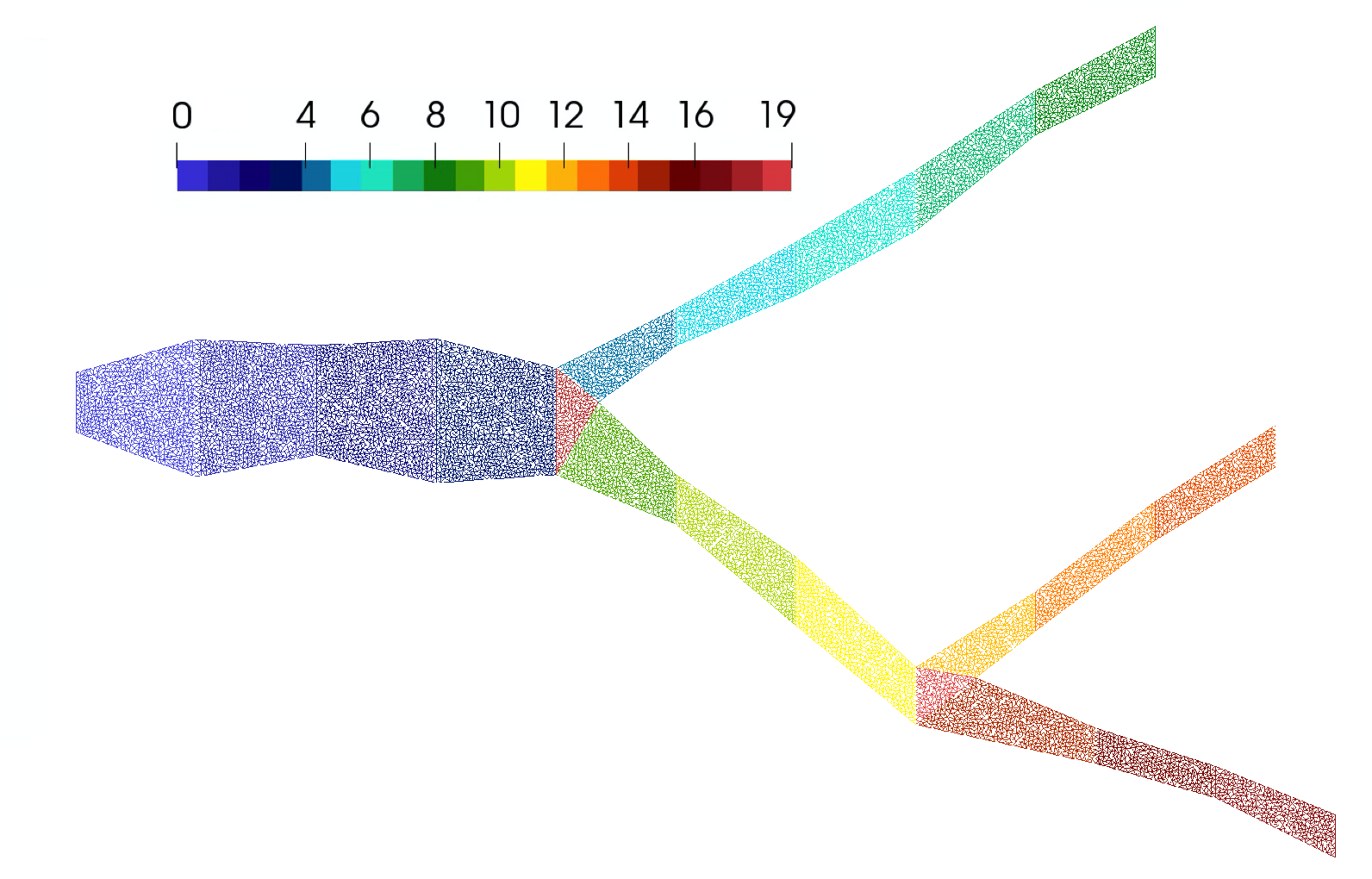
We consider a test problem with non-homogeneous Robin boundary condition for concentration with , and . We set and as initial conditions. For the inflow (left) boundary, we set for . We perform simulations for with 40 time iterations. We consider a structured and unstructured coarse grid with 10 local domains. The structured coarse grid is similar to Test 1. The unstructured grid is depicted in Figure 23, where we show local domain markers.
In Figure 24, we present reference and multiscale solutions for an unstructured grid. We depicted the magnitude of the velocity field and concentration at the final time. In multiscale solver, we used multiscale basis functions for velocity and multiscale basis functions for concentration. For reference solution, we have and . For multiscale solution, we have and . We observe a good accuracy of the presented method on an unstructured grid.
In Table 8, we present relative errors in % for velocity between reference solution and multiscale solution with different numbers of the multiscale basis functions at the final times. Results are presented for structured and unstructured grids. We observe good results for the unstructured grid, however, velocity errors are smaller on a structured grid. For example for 40 multiscale basis functions, we have % of error for a structured grid and % of error for an unstructured grid.
In Table 9, we investigate the influence of the velocity accuracy on the concentration solution for structured and unstructured coarse grids. We present numerical results for different number of multiscale basis functions for concentration of Type 2. Relative errors for concentrations are presented for four time layers with and . We can obtain good solution for concentration when we take at least 10 multiscale basis functions for velocity. For example, we obtain near 10 % of concentration error (), when we use multiscale velocity solution with 5 multiscale basis functions and near 1 % using velocity with . For concentration, we obtain similar results for structured and unstructured coarse grids using a multiscale solution of velocity with a sufficient number of basis functions.
5 Conclusions
We developed a multiscale model order reduction technique for the solution of the flow and transport problem in thin domains. Our motivation stems from reducing the problem dimension in thin layer applications. For the fine grid approximation, we apply the discontinuous Galerkin method and use the solution as a reference solution. Our multiscale approach for solving problems in complex thin geometries gives an accurate approximation of the velocity space and transport processes. We presented two types of the local multiscale basis functions for velocity and concentration, where the first is based on the approach combining all possible flows and transports directions in the local domain and the second approach is based on the separation of the macroscale parameters by the flow direction for velocity and by boundary type for transport. Moreover, our multiscale spaces can accurately capture complex processes on the rough wall boundaries with non-homogeneous boundary conditions. We use numerical simulations for three test geometries for two and three-dimensional problems to demonstrate the performance of our method. Numerical investigation of the presented method was performed (1) for different geometries of the computational domain, (2) for different boundary conditions and diffusion coefficients, and (3) for the unstructured coarse grid. The proposed multiscale method provides good results with small errors and gives a huge reduction of the system size.
References
- [1] Alfio Quarteroni and Luca Formaggia. Mathematical modelling and numerical simulation of the cardiovascular system. Handbook of numerical analysis, 12:3–127, 2004.
- [2] Abdessalem Nachit, Gregory P Panasenko, and Abdelmalek Zine. Asymptotic partial domain decomposition in thin tube structures: numerical experiments. International Journal for Multiscale Computational Engineering, 11(5), 2013.
- [3] Marie Oshima, Ryo Torii, Toshio Kobayashi, Nobuyuki Taniguchi, and Kiyoshi Takagi. Finite element simulation of blood flow in the cerebral artery. Computer methods in applied mechanics and engineering, 191(6-7):661–671, 2001.
- [4] Vincent Martin, Jérôme Jaffré, and Jean E Roberts. Modeling fractures and barriers as interfaces for flow in porous media. SIAM Journal on Scientific Computing, 26(5):1667–1691, 2005.
- [5] Luca Formaggia, Alessio Fumagalli, Anna Scotti, and Paolo Ruffo. A reduced model for darcy’s problem in networks of fractures. ESAIM: Mathematical Modelling and Numerical Analysis, 48(4):1089–1116, 2014.
- [6] Carlo D’angelo and Alfio Quarteroni. On the coupling of 1d and 3d diffusion-reaction equations: application to tissue perfusion problems. Mathematical Models and Methods in Applied Sciences, 18(08):1481–1504, 2008.
- [7] Grigory Panasenko and Konstantin Pileckas. Asymptotic analysis of the nonsteady viscous flow with a given flow rate in a thin pipe. Applicable Analysis, 91(3):559–574, 2012.
- [8] Grigory Panasenko. Method of asymptotic partial decomposition of domain for multistructures. Applicable Analysis, 96(16):2771–2779, 2017.
- [9] Thomas Y Hou and Xiao-Hui Wu. A multiscale finite element method for elliptic problems in composite materials and porous media. Journal of computational physics, 134(1):169–189, 1997.
- [10] Yalchin Efendiev and Thomas Y Hou. Multiscale finite element methods: theory and applications, volume 4. Springer Science & Business Media, 2009.
- [11] Eric T Chung and Yalchin Efendiev. Reduced-contrast approximations for high-contrast multiscale flow problems. Multiscale Modeling & Simulation, 8(4):1128–1153, 2010.
- [12] Zhiming Chen and Thomas Hou. A mixed multiscale finite element method for elliptic problems with oscillating coefficients. Mathematics of Computation, 72(242):541–576, 2003.
- [13] Jorg E Aarnes. On the use of a mixed multiscale finite element method for greaterflexibility and increased speed or improved accuracy in reservoir simulation. Multiscale Modeling & Simulation, 2(3):421–439, 2004.
- [14] Yalchin Efendiev, Juan Galvis, and Thomas Y Hou. Generalized multiscale finite element methods (gmsfem). Journal of Computational Physics, 251:116–135, 2013.
- [15] Eric Chung, Yalchin Efendiev, and Thomas Y Hou. Adaptive multiscale model reduction with generalized multiscale finite element methods. Journal of Computational Physics, 320:69–95, 2016.
- [16] Eric T Chung and Wing Tat Leung. A sub-grid structure enhanced discontinuous galerkin method for multiscale diffusion and convection-diffusion problems. Communications in Computational Physics, 14(2):370–392, 2013.
- [17] Siu Wun Cheung, Eric T Chung, and Wing Tat Leung. Constraint energy minimizing generalized multiscale discontinuous galerkin method. Journal of Computational and Applied Mathematics, page 112960, 2020.
- [18] Eric Chung, Jiuhua Hu, and Sai-Mang Pun. Convergence of the cem-gmsfem for stokes flows in heterogeneous perforated domains. arXiv preprint arXiv:2007.03237, 2020.
- [19] Todd Arbogast, Gergina Pencheva, Mary F Wheeler, and Ivan Yotov. A multiscale mortar mixed finite element method. Multiscale Modeling & Simulation, 6(1):319–346, 2007.
- [20] Patrick Jenny, Seong H Lee, and Hamdi A Tchelepi. Adaptive multiscale finite-volume method for multiphase flow and transport in porous media. Multiscale Modeling & Simulation, 3(1):50–64, 2005.
- [21] Hadi Hajibeygi, Giuseppe Bonfigli, Marc Andre Hesse, and Patrick Jenny. Iterative multiscale finite-volume method. Journal of Computational Physics, 227(19):8604–8621, 2008.
- [22] Thomas JR Hughes, Gonzalo R Feijóo, Luca Mazzei, and Jean-Baptiste Quincy. The variational multiscale method?a paradigm for computational mechanics. Computer methods in applied mechanics and engineering, 166(1-2):3–24, 1998.
- [23] Ralf Kornhuber, Daniel Peterseim, and Harry Yserentant. An analysis of a class of variational multiscale methods based on subspace decomposition. Mathematics of Computation, 87(314):2765–2774, 2018.
- [24] Axel Målqvist and Daniel Peterseim. Localization of elliptic multiscale problems. Mathematics of Computation, 83(290):2583–2603, 2014.
- [25] Assyr Abdulle, E Weinan, Björn Engquist, and Eric Vanden-Eijnden. The heterogeneous multiscale method. Acta Numerica, 21:1–87, 2012.
- [26] Bagus Putra Muljadi, Jacek Narski, Alexei Lozinski, and Pierre Degond. Nonconforming multiscale finite element method for stokes flows in heterogeneous media. part i: methodologies and numerical experiments. Multiscale Modeling & Simulation, 13(4):1146–1172, 2015.
- [27] Gaspard Jankowiak and Alexei Lozinski. Non-conforming multiscale finite element method for stokes flows in heterogeneous media. part ii: Error estimates for periodic microstructure. arXiv preprint arXiv:1802.04389, 2018.
- [28] Eric T Chung, Yalchin Efendiev, Guanglian Li, and Maria Vasilyeva. Generalized multiscale finite element methods for problems in perforated heterogeneous domains. Applicable Analysis, 95(10):2254–2279, 2016.
- [29] Eric T Chung, Wing Tat Leung, Maria Vasilyeva, and Yating Wang. Multiscale model reduction for transport and flow problems in perforated domains. Journal of Computational and Applied Mathematics, 330:519–535, 2018.
- [30] ET Chung, O Iliev, and MV Vasilyeva. Generalized multiscale finite element method for non-newtonian fluid flow in perforated domain. In AIP Conference Proceedings, volume 1773, page 100001. AIP Publishing, 2016.
- [31] Eric T Chung, Maria Vasilyeva, and Yating Wang. A conservative local multiscale model reduction technique for stokes flows in heterogeneous perforated domains. Journal of Computational and Applied Mathematics, 321:389–405, 2017.
- [32] Oleg Iliev, Zahra Lakdawala, Katherine HL Neßler, Torben Prill, Yavor Vutov, Yongfei Yang, and Jun Yao. On the pore-scale modeling and simulation of reactive transport in 3d geometries. Mathematical Modelling and Analysis, 22(5):671–694, 2017.
- [33] Ulrich Hornung and Willi Jäger. Diffusion, convection, adsorption, and reaction of chemicals in porous media. Journal of differential equations (Print), 92(2):199–225, 1991.
- [34] Grégoire Allaire, Andro Mikelić, and Andrey Piatnitski. Homogenization approach to the dispersion theory for reactive transport through porous media. SIAM Journal on Mathematical Analysis, 42(1):125–144, 2010.
- [35] Maria Vasilyeva, Eric T Chung, Wing Tat Leung, Yating Wang, and Denis Spiridonov. Upscaling method for problems in perforated domains with non-homogeneous boundary conditions on perforations using non-local multi-continuum method (nlmc). Journal of Computational and Applied Mathematics, 357:215–227, 2019.
- [36] Denis Spiridonov, Maria Vasilyeva, and Wing Tat Leung. A generalized multiscale finite element method (gmsfem) for perforated domain flows with robin boundary conditions. Journal of Computational and Applied Mathematics, 357:319–328, 2019.
- [37] Denis Spiridonov, Maria Vasilyeva, Eric T Chung, Yalchin Efendiev, and Raghavendra Jana. Multiscale model reduction of the unsaturated flow problem in heterogeneous porous media with rough surface topography. Mathematics, 8(6):904, 2020.
- [38] Eric T Chung, Yalchin Efendiev, Wing Tat Leung, Maria Vasilyeva, and Yating Wang. Non-local multi-continua upscaling for flows in heterogeneous fractured media. Journal of Computational Physics, 372:22–34, 2018.
- [39] Maria Vasilyeva, Eric T Chung, Wing Tat Leung, and Valentin Alekseev. Nonlocal multicontinuum (nlmc) upscaling of mixed dimensional coupled flow problem for embedded and discrete fracture models. GEM-International Journal on Geomathematics, 10(1):23, 2019.
- [40] Shubin Fu, Guanglian Li, Richard Craster, and Sebastien Guenneau. Wavelet-based edge multiscale finite element method for helmholtz problems in perforated domains. arXiv preprint arXiv:1906.08453, 2019.
- [41] Shubin Fu, Eric Chung, and Guanglian Li. Edge multiscale methods for elliptic problems with heterogeneous coefficients. Journal of Computational Physics, 396:228–242, 2019.
- [42] Ibrahim Y Akkutlu, Yalchin Efendiev, and Maria Vasilyeva. Multiscale model reduction for shale gas transport in fractured media. Computational Geosciences, 20(5):953–973, 2016.
- [43] Yashar Mehmani and Hamdi A Tchelepi. Multiscale formulation of two-phase flow at the pore scale. Journal of Computational Physics, 389:164–188, 2019.
- [44] Eric T Chung, Yalchin Efendiev, and Wing Tat Leung. An adaptive generalized multiscale discontinuous galerkin method for high-contrast flow problems. Multiscale Modeling & Simulation, 16(3):1227–1257, 2018.
- [45] Eric T Chung, Yalchin Efendiev, Maria Vasilyeva, and Yating Wang. A multiscale discontinuous galerkin method in perforated domains. In Proceedings of the Institute of Mathematics and Mechanics, volume 42, pages 212–229. INST MATHEMATICS & MECHANICS, NATL ACAD SCIENCES AZERBAIJAN 9 B VAHABZADEH …, 2016.
- [46] Christophe Geuzaine and Jean-François Remacle. Gmsh: A 3-d finite element mesh generator with built-in pre-and post-processing facilities. International journal for numerical methods in engineering, 79(11):1309–1331, 2009.
- [47] Anders Logg, Kent-Andre Mardal, and Garth Wells. Automated solution of differential equations by the finite element method: The FEniCS book, volume 84. Springer Science & Business Media, 2012.
- [48] Tatyana Dobroserdova, Fuyou Liang, Grigory Panasenko, and Yuri Vassilevski. Multiscale models of blood flow in the compliant aortic bifurcation. Applied Mathematics Letters, 93:98–104, 2019.