This paper was converted on www.awesomepapers.org from LaTeX by an anonymous user.
Want to know more? Visit the Converter page.

Multispace and Multilevel BDDC

Jan Mandel111Corresponding author. jan.mandel@cudenver.edu. 222Department of Mathematical Sciences, University of Colorado Denver, Denver, CO 80217-3364, USA. Supported in part by the National Science Foundation under grants CNS-0325314, DMS-071387, and CNS-0719641.    Bedřich Sousedík222Department of Mathematical Sciences, University of Colorado Denver, Denver, CO 80217-3364, USA. Supported in part by the National Science Foundation under grants CNS-0325314, DMS-071387, and CNS-0719641. 333Department of Mathematics, Faculty of Civil Engineering, Czech Technical University, Thákurova 7, 166 29 Prague 6, Czech Republic. Supported by the program of the Information society of the Academy of Sciences of the Czech Republic 1ET400760509 and by the Grant Agency of the Czech Republic GA ČR 106/08/0403.    Clark R. Dohrmann444Structural Dynamics Research Department, Sandia National Laboratories, Albuquerque NM 87185-0847, USA. Sandia is a multiprogram laboratory operated by Sandia Corporation, a Lockheed Martin Company, for the United States Department of Energy’s National Nuclear Security Administration under Contract DE-AC04-94-AL85000.
Abstract

BDDC method is the most advanced method from the Balancing family of iterative substructuring methods for the solution of large systems of linear algebraic equations arising from discretization of elliptic boundary value problems. In the case of many substructures, solving the coarse problem exactly becomes a bottleneck. Since the coarse problem in BDDC has the same structure as the original problem, it is straightforward to apply the BDDC method recursively to solve the coarse problem only approximately. In this paper, we formulate a new family of abstract Multispace BDDC methods and give condition number bounds from the abstract additive Schwarz preconditioning theory. The Multilevel BDDC is then treated as a special case of the Multispace BDDC and abstract multilevel condition number bounds are given. The abstract bounds yield polylogarithmic condition number bounds for an arbitrary fixed number of levels and scalar elliptic problems discretized by finite elements in two and three spatial dimensions. Numerical experiments confirm the theory.

AMS Subject Classification: 65N55, 65M55, 65Y05

Key words: Iterative substructuring, additive Schwarz method, balancing domain decomposition, BDD, BDDC, Multispace BDDC, Multilevel BDDC

1 Introduction

The BDDC (Balancing Domain Decomposition by Constraints) method by Dohrmann [4] is the most advanced method from the BDD family introduced by Mandel [12]. It is a Neumann-Neumann iterative substructuring method of Schwarz type [5] that iterates on the system of primal variables reduced to the interfaces between the substructures. The BDDC method is closely related to the FETI-DP method (Finite Element Tearing and Interconnecting - Dual, Primal) by Farhat et al. [6, 7]. FETI-DP is a dual method that iterates on a system for Lagrange multipliers that enforce continuity on the interfaces, with some “coarse” variables treated as primal, and it is a further development of the FETI method by Farhat and Roux [8]. Polylogarithmic condition number estimates for BDDC were obtained in [13, 14] and a proof that the eigenvalues of BDDC and FETI-DP are actually the same except for eigenvalue equal to one was given in Mandel et al. [14]. Simpler proofs of the equality of eigenvalues were obtained by Li and Widlund [10], and also by Brenner and Sung [3], who also gave an example when BDDC has an eigenvalue equal to one but FETI-DP does not. In the case of many substructures, solving the coarse problem exactly becomes a bottleneck. However, since the coarse problem in BDDC has the same form as the original problem, the BDDC method can be applied recursively to solve the coarse problem only approximately. This leads to a multilevel form of BDDC in a straightforward manner, see Dohrmann [4]. Polylogarithmic condition number bounds for three-level BDDC (BDDC with two coarse levels) were proved in two and three spatial dimensions by Tu [20, 19].

In this paper, we present a new abstract Multispace BDDC method. The method extends a simple variational setting of BDDC from Mandel and Sousedík [15], which could be understood as an abstract version of BDDC by partial subassembly in Li and Widlund [11]. However, we do not adopt their change of variables, which does not seem to be suitable in our abstract setting. We provide a condition number estimate for the abstract Multispace BDDC method, which generalizes the estimate for a single space from [15]. The proof is based on the abstract additive Schwarz theory by Dryja and Widlund [5]. Many BDDC formulations (with an explicit treatment of substructure interiors, after reduction to substructure interfaces, with two levels, and multilevel) are then viewed as abstract Multispace BDDC with a suitable choice of spaces and operators, and abstract condition number estimates for those BDDC methods follow. This result in turn gives a polylogarithmic condition number bound for Multilevel BDDC applied to a second-order scalar elliptic model problems, with an arbitrary number of levels. A brief presentation of the main results of the paper, without proofs and with a simplified formulation of the Multispace BDDC estimate, is contained in the conference paper [16].

The paper is organized as follows. In Sec. 2 we introduce the abstract problem setting. In Sec. 3 we formulate an abstract Multispace BDDC as an additive Schwarz preconditioner. In Sec. 4 we introduce the settings of a model problem using finite element discretization. In Sec. 5 we recall the algorithm of the original (two-level) BDDC method and formulate it as a Multispace BDDC. In Sec. 6 we generalize the algorithm to obtain Multilevel BDDC and we also give an abstract condition number bound. In Sec. 7 we derive the condition number bound for the model problem. Finally, in Sec. 8, we report on numerical results.

2 Abstract Problem Setting

We wish to solve an abstract linear problem

uX:a(u,v)=fX,v,vX,u\in X:a(u,v)=\left\langle f_{X},v\right\rangle,\quad\forall v\in X, (1)

where XX is a finite dimensional linear space, a(,)a\left(\cdot,\cdot\right) is a symmetric positive definite bilinear form defined on XX, fXXf_{X}\in X^{\prime} is the right-hand side with XX^{\prime} denoting the dual space of XX, and ,\left\langle\cdot,\cdot\right\rangle is the duality pairing. The form a(,)a\left(\cdot,\cdot\right) is also called the energy inner product, the value of the quadratic form a(u,u)a\left(u,u\right) is called the energy of uu, and the norm ua=a(u,u)1/2\left\|u\right\|_{a}=a\left(u,u\right)^{1/2} is called the energy norm. The operator AX:XXA_{X}:X\mapsto X^{\prime} associated with aa is defined by

a(u,v)=AXu,v,u,vX.a(u,v)=\left\langle A_{X}u,v\right\rangle,\quad\forall u,v\in X.

A preconditioner is a mapping B:XXB:X^{\prime}\rightarrow X and we will look for preconditioners such that r,Br\left\langle r,Br\right\rangle is also symmetric and positive definite on XX^{\prime}. It is well known that then BAX:XXBA_{X}:X\rightarrow X has only real positive eigenvalues, and convergence of the preconditioned conjugate gradients method is bounded using the condition number

κ=λmax(BAX)λmin(BAX),\kappa=\frac{\lambda_{\max}(BA_{X})}{\lambda_{\min}(BA_{X})},

which we wish to bound above.

All abstract spaces in this paper are finite dimensional linear spaces and we make no distinction between a linear operator and its matrix.

3 Abstract Multispace BDDC

To introduce abstract Multispace BDDC preconditioner, suppose that the bilinear form aa is defined and symmetric positive semidefinite on some larger space WXW\supset X. The preconditioner is derived from the abstract additive Schwarz theory, however we decompose some space between XX and WW rather than XX as it would be done in the additive Schwarz method: In the design of the preconditioner, we choose spaces VkV_{k}, k=1,,Mk=1,\ldots,M, such that

Xk=1MVkW.X\subset\sum_{k=1}^{M}V_{k}\subset W. (2)
Assumption 1

The form a(,)a\left(\cdot,\cdot\right) is positive definite on each VkV_{k} separately.

Algorithm 2 (Abstract Multispace BDDC)

Given spaces VkV_{k} and linear operators QkQ_{k}, k=1,,Mk=1,\ldots,M such that a(,)a\left(\cdot,\cdot\right) is positive definite on each space VkV_{k}, and

Xk=1MVk,Qk:VkX,X\subset\sum_{k=1}^{M}V_{k},\quad Q_{k}:V_{k}\rightarrow X,

define the preconditioner B:rXuXB:r\in X^{\prime}\longmapsto u\in X by

B:ru=k=1MQkvk,vkVk:a(vk,zk)=r,Qkzk,zkVk.B:r\mapsto u=\sum_{k=1}^{M}Q_{k}v_{k},\quad v_{k}\in V_{k}:\quad a\left(v_{k},z_{k}\right)=\left\langle r,Q_{k}z_{k}\right\rangle,\quad\forall z_{k}\in V_{k}. (3)

We formulate the condition number bound first in the full strength allowed by the proof. The bound used in the rest of this paper will be a corollary.

Theorem 3

Define for all k=1,,Mk=1,\ldots,M the spaces VkV_{k}^{\mathcal{M}} by

Vk={vkVk:zkVk:Qkvk=Qkzkvka2zka2}.V_{k}^{\mathcal{M}}=\left\{v_{k}\in V_{k}:\forall z_{k}\in V_{k}:Q_{k}v_{k}=Q_{k}z_{k}\Longrightarrow\left\|v_{k}\right\|_{a}^{2}\leq\left\|z_{k}\right\|_{a}^{2}\right\}.

If there exist constants C0,C_{0}, ω,\omega, and a symmetric matrix =(eij)i,j=1M\mathcal{E}=(e_{ij})_{i,j=1}^{M}, such that

uXvkVk, k=1,,M:u=k=1MQkvk, k=1Mvka2C0ua2\displaystyle\forall u\in X\quad\exists v_{k}\in V_{k},\text{ }k=1,\ldots,M:u=\sum_{k=1}^{M}Q_{k}v_{k},\text{ }\sum_{k=1}^{M}\left\|v_{k}\right\|_{a}^{2}\leq C_{0}\left\|u\right\|_{a}^{2} (4)
k=1,,MvkVk:Qkvka2ωvka2\displaystyle\forall k=1,\ldots,M\quad\forall v_{k}\in V_{k}^{\mathcal{M}}:\left\|Q_{k}v_{k}\right\|_{a}^{2}\leq\omega\left\|v_{k}\right\|_{a}^{2} (5)
zkQkVk, k=1,,M:a(zi,zj)eijziazja,\displaystyle\forall z_{k}\in Q_{k}V_{k},\text{ }k=1,\ldots,M:a\left(z_{i},z_{j}\right)\leq e_{ij}\left\|z_{i}\right\|_{a}\left\|z_{j}\right\|_{a},\quad (6)

then the preconditioner from Algorithm 2 satisfies

κ=λmax(BAX)λmin(BAX)C0ωρ().\kappa=\frac{\lambda_{\max}(BA_{X})}{\lambda_{\min}(BA_{X})}\leq C_{0}\omega\rho(\mathcal{E}).

Proof. We interpret the Multispace BDDC preconditioner as an abstract additive Schwarz method. An abstract additive Schwarz method is specified by a decomposition of the space XX into subspaces,

X=X1++XM,X=X_{1}+...+X_{M}, (7)

and by symmetric positive definite bilinear forms bib_{i} on XiX_{i}. The preconditioner is a linear operator

B:XX,B:ru,B:X^{\prime}\rightarrow X,\qquad B:r\mapsto u,

defined by solving the following variational problems on the subspaces and adding the results,

B:ru=k=1Muk,ukXk:bk(uk,yk)=r,yk,ykXk.B:r\mapsto u=\sum\limits_{k=1}^{M}u_{k},\quad u_{k}\in X_{k}:\quad b_{k}(u_{k},y_{k})=\left\langle r,y_{k}\right\rangle,\quad\forall y_{k}\in X_{k}. (8)

Dryja and Widlund [5] proved that if there exist constants C0,C_{0}, ω,\omega, and a symmetric matrix =(eij)i,j=1M\mathcal{E}=(e_{ij})_{i,j=1}^{M}, such that

u\displaystyle\forall u X ukXk, k=1,,M:u=k=1Muk, k=1Mukbk2C0ua2\displaystyle\in X\text{ }\exists u_{k}\in X_{k},\text{ }k=1,\ldots,M:u=\sum_{k=1}^{M}u_{k},\text{ }\sum_{k=1}^{M}\left\|u_{k}\right\|_{b_{k}}^{2}\leq C_{0}\left\|u\right\|_{a}^{2} (9)
k\displaystyle\forall k =1,,M ukXk:uka2ωukbk2\displaystyle=1,\ldots,M\text{ }\forall u_{k}\in X_{k}:\left\|u_{k}\right\|_{a}^{2}\leq\omega\left\|u_{k}\right\|_{b_{k}}^{2} (10)
uk\displaystyle\forall u_{k} Xk, k=1,,M:a(ui,uj)eijuiauja\displaystyle\in X_{k},\text{ }k=1,\ldots,M:a(u_{i},u_{j})\leq e_{ij}\left\|u_{i}\right\|_{a}\left\|u_{j}\right\|_{a} (11)

then

κ=λmax(BAX)λmin(BAX)C0ωρ(),\kappa=\frac{\lambda_{\max}(BA_{X})}{\lambda_{\min}(BA_{X})}\leq C_{0}\omega\rho(\mathcal{E}),

where ρ\rho is the spectral radius.

Now the idea of the proof is essentially to map the assumptions of the abstract additive Schwarz estimate from the decomposition (7) of the space XX to the decomposition (2). Define the spaces

Xk=QkVk.X_{k}=Q_{k}V_{k}.

We will show that the preconditioner (3) satisfies (8), where bkb_{k} is defined by

bk(uk,yk)=a(Gkx,Gkz),x,zX,uk=QkGkx,yk=QkGkz.b_{k}(u_{k},y_{k})=a\left(G_{k}x,G_{k}z\right),\quad x,z\in X,\quad u_{k}=Q_{k}G_{k}x,\quad y_{k}=Q_{k}G_{k}z. (12)

with the operators Gk:XVkG_{k}:X\rightarrow V_{k}^{\mathcal{M}} defined by

Gk:uvk,12a(vk,vk)min, s.t. vkVk, u=k=1MQkvk,G_{k}:u\mapsto v_{k},\quad\frac{1}{2}a\left(v_{k},v_{k}\right)\rightarrow\min,\text{ s.t. }v_{k}\in V_{k}^{\mathcal{M}},\text{ }u=\sum_{k=1}^{M}Q_{k}v_{k}, (13)

First, from the definition of operators GkG_{k}, spaces Xk,X_{k}, and because aa is positive definite on VkV_{k} by Assumption (1), it follows that GkxG_{k}x and GkzG_{k}z in (12) exist and are unique, so bkb_{k} is defined correctly. To prove (8), let vkv_{k} be as in (3) and note that vkv_{k} is the solution of

12a(vk,vk)r,Qkvkmin,vkVk.\frac{1}{2}a\left(v_{k},v_{k}\right)-\left\langle r,Q_{k}v_{k}\right\rangle\rightarrow\min,\quad v_{k}\in V_{k}.

Consequently, the preconditioner (3) is an abstract additive Schwarz method and we only need to verify the inequalities (9)–(11). To prove (9), let uXu\in X. Then, with vkv_{k} from the assumption (4) and with uk=QkGkvku_{k}=Q_{k}G_{k}v_{k} as in (12), it follows that

u=k=1Muk,k=1Mukbk2=k=1Mvka2C0ua2.u=\sum_{k=1}^{M}u_{k},\quad\sum_{k=1}^{M}\left\|u_{k}\right\|_{b_{k}}^{2}=\sum_{k=1}^{M}\left\|v_{k}\right\|_{a}^{2}\leq C_{0}\left\|u\right\|_{a}^{2}.

Next, let ukXku_{k}\in X_{k}. From the definitions of XkX_{k} and VkV_{k}^{\mathcal{M}}, it follows that there exist unique vkVkv_{k}\in V_{k}^{\mathcal{M}} such that uk=Qkvku_{k}=Q_{k}v_{k}. Using the assumption (5) and the definition of bkb_{k} in (12), we get

uka2=Qkvka2ωvka2=ωukbk2,\left\|u_{k}\right\|_{a}^{2}=\left\|Q_{k}v_{k}\right\|_{a}^{2}\leq\omega\left\|v_{k}\right\|_{a}^{2}=\omega\left\|u_{k}\right\|_{b_{k}}^{2},

which gives (10). Finally, (6) is the same as (11).   

The next Corollary was given without proof in [16, Lemma 1]. This is the special case of Theorem 3 that will be actually used. In the case when M=1M=1, this result was proved in [15].

Corollary 4

Assume that the subspaces VkV_{k} are energy orthogonal, the operators QkQ_{k} are projections, a(,)a\left(\cdot,\cdot\right) is positive definite on each space VkV_{k}, and

uX:[u=k=1Mvk,vkVk]u=k=1MQkvk.\forall u\in X:\left[u=\sum_{k=1}^{M}v_{k},\ v_{k}\in V_{k}\right]\Longrightarrow u=\sum_{k=1}^{M}Q_{k}v_{k}\text{.} (14)

Then the abstract Multispace BDDC preconditioner from Algorithm 2 satisfies

κ=λmax(BAX)λmin(BAX)ω=maxksupvkVkQkvka2vka2 .{\kappa=\frac{\lambda_{\max}(BA_{X})}{\lambda_{\min}(BA_{X})}\leq\omega=\max_{k}\sup_{v_{k}\in V_{k}}\frac{\left\|Q_{k}v_{k}\right\|_{a}^{2}}{\left\|v_{k}\right\|_{a}^{2}}}\text{ }{.} (15)

Proof. We only need to verify the assumptions of Theorem 3. Let uXu\in X and choose vkv_{k} as the energy orthogonal projections of uu on VkV_{k}. First, since the spaces VkV_{k} are energy orthogonal, u=vku={\textstyle\sum}v_{k}, QkQ_{k} are projections, and from (14) u=Qkvku={\textstyle\sum}Q_{k}v_{k}, we get that ua2=vka2\left\|u\right\|_{a}^{2}={\textstyle\sum}\left\|v_{k}\right\|_{a}^{2} which proves (4) with C0=1C_{0}=1. Next, the assumption (5) becomes the definition of ω{\omega} in (15). Finally, (6) with =I\mathcal{E}=I follows from the orthogonality of subspaces VkV_{k}.   

Remark 5

The assumption (14) can be written as

k=1MQkPk|X=I,\left.\sum_{k=1}^{M}Q_{k}P_{k}\right|_{X}=I,

where PkP_{k} is the aa-orthogonal projection from j=1MVj\bigoplus\nolimits_{j=1}^{M}V_{j} onto VkV_{k}. Hence, the property (14) is a type of decomposition of unity.

In the case when M=1M=1, (14) means that the projection Q1Q_{1} is onto XX.

4 Finite Element Problem Setting

Let Ω\Omega be a bounded domain in d\mathbb{R}^{d}, d=2d=2 or 33, decomposed into NN nonoverlapping subdomains Ωs\Omega^{s}, s=1,,Ns=1,...,N, which form a conforming triangulation of the domain Ω\Omega. Subdomains will be also called substructures. Each substructure is a union of Lagrangian P1P1 or Q1Q1 finite elements with characteristic mesh size hh, and the nodes of the finite elements between substructures coincide. The nodes contained in the intersection of at least two substructures are called boundary nodes. The union of all boundary nodes is called the interface Γ\Gamma. The interfaceΓ~\Gamma is a union of three different types of open sets: faces, edges, and vertices. The substructure vertices will be also called corners. For the case of regular substructures, such as cubes or tetrahedrons, we can use standard geometric definition of faces, edges, and vertices; cf., e.g., [9] for a more general definition.

In this paper, we find it more convenient to use the notation of abstract linear spaces and linear operators between them instead of the space n\mathbb{R}^{n} and matrices. The results can be easily converted to the matrix language by choosing a finite element basis. The space of the finite element functions on Ω\Omega will be denoted as UU. Let WsW^{s} be the space of finite element functions on substructure Ωs\Omega^{s}, such that all of their degrees of freedom on ΩsΩ\partial\Omega^{s}\cap\partial\Omega are zero. Let

W=W1××WN,W=W^{1}\times\cdots\times W^{N},

and consider a bilinear form arising from the second-order scalar elliptic problem as

a(u,v)=s=1NΩSuvdx,u,vW.a\left(u,v\right)=\sum_{s=1}^{N}\int_{\Omega^{S}}\nabla u\nabla v\,dx,\quad u,v\in W. (16)

Now UWU\subset W is the subspace of all functions from WW that are continuous across the substructure interfaces. We are interested in the solution of the problem (1) with X=UX=U,

uU:a(u,v)=f,v,vU,u\in U:a(u,v)=\left\langle f,v\right\rangle,\quad\forall v\in U, (17)

where the bilinear form aa is associated on the space UU with the system operatorA~A, defined by

A:UU,a(u,v)=Au,v for all u,vU,A:U\mapsto U^{\prime},\quad a(u,v)=\left\langle Au,v\right\rangle\text{ for all }u,v\in U, (18)

and fUf\in U^{\prime} is the right-hand side. Hence, (17) is equivalent to

Au=f.Au=f. (19)

Define UIUU_{I}\subset U as the subspace of functions that are zero on the interface Γ\Gamma, i.e., the “interior” functions. Denote by PP the energy orthogonal projection from WW onto UIU_{I},

P:wWvIUI:a(vI,zI)=a(w,zI),zIUI.P:w\in W\longmapsto v_{I}\in U_{I}:a\left(v_{I},z_{I}\right)=a\left(w,z_{I}\right),\quad\forall z_{I}\in U_{I}.

Functions from (IP)W\left(I-P\right)W, i.e., from the nullspace of P,P, are called discrete harmonic; these functions are aa-orthogonal to UIU_{I} and energy minimal with respect to increments in UIU_{I}. Next, let W^\widehat{W} be the space of all discrete harmonic functions that are continuous across substructure boundaries, that is

W^=(IP)U.\widehat{W}=\left(I-P\right)U. (20)

In particular,

U=UIW^,UIaW^.U=U_{I}\oplus\widehat{W},\quad U_{I}\perp_{a}\widehat{W}. (21)

A common approach in substructuring is to reduce the problem to the interface. The problem (17) is equivalent to two independent problems on the energy orthogonal subspaces UIU_{I} and W^\widehat{W}, and the solution uu satisfies u=uI+u^u=u_{I}+\widehat{u}, where

u\displaystyle u UI:a(uI,vI)=f,vI,vIUI,\displaystyle\in U_{I}:a(u_{I},v_{I})=\left\langle f,v_{I}\right\rangle,\quad\forall v_{I}\in U_{I}, (22)
u\displaystyle u W^:a(u^,v^)=f,v^,v^W^.\displaystyle\in\widehat{W}:a(\widehat{u},\widehat{v})=\left\langle f,\widehat{v}\right\rangle,\quad\forall\widehat{v}\in\widehat{W}. (23)

The solution of the interior problem (22) decomposes into independent problems, one per each substructure. The reduced problem (23) is then solved by preconditioned conjugate gradients. The reduced problem (23) is usually written equivalently as

uW^:s(u^,v^)=g,v^,v^W^,u\in\widehat{W}:s(\widehat{u},\widehat{v})=\left\langle g,\widehat{v}\right\rangle,\quad\forall\widehat{v}\in\widehat{W},

where ss is the form aa restricted on the subspace W^\widehat{W}, and gg is the reduced right hand side, i.e., the functional ff restricted to the space W^\widehat{W}. The reduced right-hand side gg is usually written as

g,v^=f,v^a(uI,v^),v^W^,\left\langle g,\widehat{v}\right\rangle=\left\langle f,\widehat{v}\right\rangle-a(u_{I},\widehat{v}),\quad\forall\widehat{v}\in\widehat{W}, (24)

because a(uI,v^)=0a(u_{I},\widehat{v})=0 by (21). In the implementation, the process of passing to the reduced problem becomes the elimination of the internal degrees of freedom of the substructures, also known as static condensation. The matrix of the reduced bilinear form ss in the basis defined by interface degrees of freedom becomes the Schur complement, and (24) becomes the reduced right-hand side. For details on the matrix formulation, see, e.g., [17, Sec. 4.6] or [18, Sec. 4.3].

The BDDC method is a two-level preconditioner characterized by the selection of certain coarse degrees of freedom, such as values at the corners and averages over edges or faces of substructures. Define W~W\widetilde{W}\subset W as the subspace of all functions such that the values of any coarse degrees of freedom have a common value for all relevant substructures and vanish on Ω,\partial\Omega, and W~ΔW\widetilde{W}_{\Delta}\subset W as the subspace of all function such that their coarse degrees of freedom vanish. Next, define W~Π\widetilde{W}_{\Pi} as the subspace of all functions such that their coarse degrees of freedom between adjacent substructures coincide, and such that their energy is minimal. Clearly, functions in W~Π\widetilde{W}_{\Pi} are uniquely determined by the values of their coarse degrees of freedom, and

W~ΔaW~Π, and W~=W~ΔW~Π.\widetilde{W}_{\Delta}\perp_{a}\widetilde{W}_{\Pi},\text{\quad and\quad}\widetilde{W}=\widetilde{W}_{\Delta}\oplus\widetilde{W}_{\Pi}. (25)

We assume that

a is positive definite on W~.a\text{ is positive definite on }\widetilde{W}. (26)

That is the case when aa is positive definite on the space UU, where the problem (1) is posed, and there are sufficiently many coarse degrees of freedom. We further assume that the coarse degrees of freedom are zero on all functions from UIU_{I}, that is,

UIW~Δ.U_{I}\subset\widetilde{W}_{\Delta}. (27)

In other words, the coarse degrees of freedom depend on the values on substructure boundaries only. From (25) and (27), it follows that the functions in W~Π\widetilde{W}_{\Pi} are discrete harmonic, that is,

W~Π=(IP)W~Π.\widetilde{W}_{\Pi}=\left(I-P\right)\widetilde{W}_{\Pi}. (28)

Next, let EE be a projection from W~\widetilde{W} onto UU, defined by taking some weighted average on substructure interfaces. That is, we assume that

E:W~U,EU=U,E2=E.E:\widetilde{W}\rightarrow U,\quad EU=U,\quad E^{2}=E. (29)

Since a projection is the identity on its range, it follows that EE does not change the interior degrees of freedom,

EUI=UI,EU_{I}=U_{I}, (30)

since UIUU_{I}\subset U. Finally, we show that the operator (IP)E\left(I-P\right)E is a projection. From (30) it follows that EE does not change interior degrees of freedom, so EP=PEP=P. Then, using the fact that IPI-P and EE are projections, we get

[(IP)E]2\displaystyle\left[\left(I-P\right)E\right]^{2} =(IP)E(IP)E\displaystyle=\left(I-P\right)E\left(I-P\right)E
=(IP)(EP)E\displaystyle=\left(I-P\right)\left(E-P\right)E (31)
=(IP)(IP)E=(IP)E.\displaystyle=\left(I-P\right)\left(I-P\right)E=\left(I-P\right)E.
Remark 6

In [14, 15], the whole analysis was done in spaces of discrete harmonic functions after eliminating UIU_{I}, and the space W^\widehat{W} was the solution space. In particular, W~\widetilde{W} consisted of discrete harmonic functions only, while the same space here would be (IP)W~(I-P)\widetilde{W}. The decomposition of this space used in [14, 15] would be in our context written as

(IP)W~=(IP)W~ΔW~Π,(IP)W~ΔaW~Π.(I-P)\widetilde{W}=(I-P)\widetilde{W}_{\Delta}\oplus\widetilde{W}_{\Pi},\quad(I-P)\widetilde{W}_{\Delta}\perp_{a}\widetilde{W}_{\Pi}. (32)

In the next section, the space XX will be either UU or W^\widehat{W}.

5 Two-level BDDC as Multispace BDDC

We show several different ways the original, two-level, BDDC algorithm can be interpreted as multispace BDDC. We consider first BDDC applied to the reduced problem (23), that is, (1) with X=W^X=\widehat{W}. This was the formulation considered in [14]. Define the space of discrete harmonic functions with coarse degrees of freedom continuous across the interface

W~Γ=(IP)W~.\widetilde{W}_{\Gamma}=\left(I-P\right)\widetilde{W}.

Because we work in the space of discrete harmonic functions and the output of the averaging operator EE is not discrete harmonic, denote

EΓ=(IP)E.E_{\Gamma}=\left(I-P\right)E. (33)

In an implementation, discrete harmonic functions are represented by the values of their degrees of freedom on substructure interfaces, cf., e.g. [18]; hence, the definition (33) serves formal purposes only, so that everything can be written in terms of discrete harmonic functions without passing to the matrix formulation.

Algorithm 7 ([15], BDDC on the reduced problem)

Define the preconditioner rW^uW^r\in\widehat{W}^{\prime}\longmapsto u\in\widehat{W} by

u=EΓwΓ,wΓW~Γ:a(wΓ,zΓ)=r,EΓzΓ,zΓW~Γ.u=E_{\Gamma}w_{\Gamma},\quad w_{\Gamma}\in\widetilde{W}_{\Gamma}:a\left(w_{\Gamma},z_{\Gamma}\right)=\left\langle r,E_{\Gamma}z_{\Gamma}\right\rangle,\quad\forall z_{\Gamma}\in\widetilde{W}_{\Gamma}. (34)
Proposition 8 ([15])

The BDDC preconditioner on the reduced problem in Algorithm 7 is the abstract Multispace BDDC from Algorithm 2 with M=1M=1 and the space and operator given by

X=W^,V1=W~Γ,Q1=EΓ.X=\widehat{W},\quad V_{1}=\widetilde{W}_{\Gamma},\quad Q_{1}=E_{\Gamma}. (35)

Also, the assumptions of Corollary 4 are satisfied.

Proof. We only need to note that the bilinear form a(,)a(\cdot,\cdot) is positive definite on W~ΓW~\widetilde{W}_{\Gamma}\subset\widetilde{W} by (26), and the operator EΓE_{\Gamma} defined by (33) is a projection by (31). The projection EΓE_{\Gamma} is onto W^\widehat{W} because EE is onto UU by (29), and IPI-P maps UU onto W^\widehat{W} by the definition of W^\widehat{W} in (20).   

Using the decomposition (32), we can split the solution in the space W~Γ\widetilde{W}_{\Gamma} into the independent solution of two subproblems: mutually independent problems on substructures as the solution in the space W~ΓΔ=(IP)W~Δ\widetilde{W}_{\Gamma\Delta}=(I-P)\widetilde{W}_{\Delta}, and a solution of global coarse problem in the space W~Π\widetilde{W}_{\Pi}. The space W~Γ\widetilde{W}_{\Gamma} has a decomposition

W~Γ=W~ΓΔW~Π, and W~ΓΔaW~Π,\widetilde{W}_{\Gamma}=\widetilde{W}_{\Gamma\Delta}\oplus\widetilde{W}_{\Pi},\text{\quad and\quad}\widetilde{W}_{\Gamma\Delta}\perp_{a}\widetilde{W}_{\Pi}, (36)

the same as the decomposition (32), and Algorithm 7 can be rewritten as follows.

Algorithm 9 ([14], BDDC on the reduced problem)

Define the preconditioner rW^uW^r\in\widehat{W}^{\prime}\longmapsto u\in\widehat{W} by u=EΓ(wΓΔ+wΠ)u=E_{\Gamma}\left(w_{\Gamma\Delta}+w_{\Pi}\right), where

wΓΔ\displaystyle w_{\Gamma\Delta} W~ΓΔ:a(wΓΔ,zΓΔ)=r,EΓzΓΔ,zΓΔW~ΓΔ,\displaystyle\in\widetilde{W}_{\Gamma\Delta}:a\left(w_{\Gamma\Delta},z_{\Gamma\Delta}\right)=\left\langle r,E_{\Gamma}z_{\Gamma\Delta}\right\rangle,\quad\forall z_{\Gamma\Delta}\in\widetilde{W}_{\Gamma\Delta}, (37)
wΠ\displaystyle w_{\Pi} W~Π:a(wΠ,zΓΠ)=r,EΓzΓΠ,zΓΠW~Π.\displaystyle\in\widetilde{W}_{\Pi}:a\left(w_{\Pi},z_{\Gamma\Pi}\right)=\left\langle r,E_{\Gamma}z_{\Gamma\Pi}\right\rangle,\quad\forall z_{\Gamma\Pi}\in\widetilde{W}_{\Pi}. (38)
Proposition 10

The BDDC preconditioner on the reduced problem in Algorithm 9 is the abstract Multispace BDDC from Algorithm 2 with M=2M=2 and the spaces and operators given by

X=W^,V1=W~ΓΔ,V2=W~Π,Q1=Q2=EΓ.X=\widehat{W},\quad V_{1}=\widetilde{W}_{\Gamma\Delta},\quad V_{2}=\widetilde{W}_{\Pi},\quad Q_{1}=Q_{2}=E_{\Gamma}. (39)

Also, the assumptions of Corollary 4 are satisfied.

Proof. Let rW^r\in\widehat{W}^{\prime}. Define the vectors viv_{i}, i=1,2i=1,2 in Multispace BDDC by (3) with ViV_{i} and QiQ_{i} given by (39). Let u,u, wΓΔ,w_{\Gamma\Delta}, wΠw_{\Pi} be the quantities in Algorithm 9, defined by (37)-(38). Using the decomposition (36), any wΓW~Γw_{\Gamma}\in\widetilde{W}_{\Gamma} can be written uniquely as wΓ=wΓΔw_{\Gamma}=w_{\Gamma\Delta}+wΠw_{\Pi} for some wΓΔw_{\Gamma\Delta} and wΠw_{\Pi} corresponding to (3) as v1=wΓΔv_{1}=w_{\Gamma\Delta} and v2=wΠv_{2}=w_{\Pi}, and u=EΓ(wΓΔ+wΠ)u=E_{\Gamma}\left(w_{\Gamma\Delta}+w_{\Pi}\right).

To verify the assumptions of Corollary 4, note that the decomposition (36) is aa-orthogonal, a(,)a(\cdot,\cdot) is positive definite on both W~ΓΔ\widetilde{W}_{\Gamma\Delta} and W~Π\widetilde{W}_{\Pi} as subspaces of W~Γ\widetilde{W}_{\Gamma} by (26), and EΓE_{\Gamma} is a projection by (31).   

Next, we present a BDDC formulation on the space UU with explicit treatment of interior functions in the space UIU_{I} as in [4, 13], i.e., in the way the BDDC algorithm was originally formulated.

Algorithm 11 ([4, 13], original BDDC)

Define the preconditioner rUuUr\in U^{\prime}\longmapsto u\in U as follows. Compute the interior pre-correction

uIUI:a(uI,zI)=r,zI,zIUI.u_{I}\in U_{I}:a\left(u_{I},z_{I}\right)=\left\langle r,z_{I}\right\rangle,\quad\forall z_{I}\in U_{I}. (40)

Set up the updated residual

rBU,rB,v=r,va(uI,v),vU.r_{B}\in U^{\prime},\quad\left\langle r_{B},v\right\rangle=\left\langle r,v\right\rangle-a\left(u_{I},v\right),\quad\forall v\in U. (41)

Compute the substructure correction

uΔ=EwΔ,wΔW~Δ:a(wΔ,zΔ)=rB,EzΔ,zΔW~Δ.u_{\Delta}=Ew_{\Delta},\quad w_{\Delta}\in\widetilde{W}_{\Delta}:a\left(w_{\Delta},z_{\Delta}\right)=\left\langle r_{B},Ez_{\Delta}\right\rangle,\quad\forall z_{\Delta}\in\widetilde{W}_{\Delta}. (42)

Compute the coarse correction

uΠ=EwΠ,wΠW~Π:a(wΠ,zΠ)=rB,EzΠ,zΠW~Π.u_{\Pi}=Ew_{\Pi},\quad w_{\Pi}\in\widetilde{W}_{\Pi}:a\left(w_{\Pi},z_{\Pi}\right)=\left\langle r_{B},Ez_{\Pi}\right\rangle,\quad\forall z_{\Pi}\in\widetilde{W}_{\Pi}. (43)

Add the corrections

uB=uΔ+uΠ.u_{B}=u_{\Delta}+u_{\Pi}.

Compute the interior post-correction

vIUI:a(vI,zI)=a(uB,zI),zIUI.v_{I}\in U_{I}:a\left(v_{I},z_{I}\right)=a\left(u_{B},z_{I}\right),\quad\forall z_{I}\in U_{I}. (44)

Apply the combined corrections

u=uBvI+uI.u=u_{B}-v_{I}+u_{I}. (45)

The interior corrections (40) and (44) decompose into independent Dirichlet problems, one for each substructure. The substructure correction (42) decomposes into independent constrained Neumann problems, one for each substructure. Thus, the evaluation of the preconditioner requires three problems to be solved in each substructure, plus solution of the coarse problem (43). In addition, the substructure corrections can be solved in parallel with the coarse problem.

Remark 12

As it is well known [4], the first interior correction (40) can be omitted in the implementation by starting the iterations from an initial solution such that the residual in the interior of the substructures is zero,

a(u,zI)fX,zI=0,zIUI,a\left(u,z_{I}\right)-\left\langle f_{X},z_{I}\right\rangle=0,\quad\forall z_{I}\in U_{I},

i.e., such that the error is discrete harmonic. Then the output of the preconditioner is discrete harmonic and thus the errors in all the CG iterations (which are linear combinations of the original error and outputs from the preconditioner) are also discrete harmonic by induction.

The following proposition will be the starting point for the multilevel case.

Proposition 13

The original BDDC preconditioner in Algorithm 11 is the abstract Multispace BDDC from Algorithm 2 with M=3M=3 and the spaces and operators given by

X\displaystyle X =U,V1=UI,V2=(IP)W~Δ,V3=W~Π,\displaystyle=U,\quad V_{1}=U_{I},\quad V_{2}=(I-P)\widetilde{W}_{\Delta},\quad V_{3}=\widetilde{W}_{\Pi}, (46)
Q1\displaystyle Q_{1} =I,Q2=Q3=(IP)E,\displaystyle=I,\quad Q_{2}=Q_{3}=\left(I-P\right)E, (47)

and the assumptions of Corollary 4 are satisfied.

Proof. Let rUr\in U^{\prime}. Define the vectors viv_{i}, i=1,2,3i=1,2,3, in Multispace BDDC by (3) with the spaces ViV_{i} given by (46) and with the operators QiQ_{i} given by (47). Let uIu_{I}, rBr_{B}, wΔw_{\Delta}, wΠw_{\Pi}, uBu_{B}, vIv_{I}, and uu be the quantities in Algorithm 11, defined by (40)-(45).

First, with V1=UIV_{1}=U_{I}, the definition of v1v_{1} in (3) with k=1k=1 is identical to the definition of uIu_{I} in (40), so uI=v1u_{I}=v_{1}.

Next, consider wΔW~Δw_{\Delta}\in\widetilde{W}_{\Delta} defined in (42). We show that wΔw_{\Delta} satisfies (3) with k=2k=2, i.e., v2=wΔv_{2}=w_{\Delta}. So, let zΔW~Δz_{\Delta}\in\widetilde{W}_{\Delta} be arbitrary. From (42) and (41),

a(wΔ,zΔ)=rB,EzΔ=r,EzΔa(uI,EzΔ).a\left(w_{\Delta},z_{\Delta}\right)=\left\langle r_{B},Ez_{\Delta}\right\rangle=\left\langle r,Ez_{\Delta}\right\rangle-a\left(u_{I},Ez_{\Delta}\right). (48)

Now from the definition of uIu_{I} by (40) and the fact that PEzΔUIPEz_{\Delta}\in U_{I}, we get

r,PEzΔa(uI,PEzΔ)=0,\left\langle r,PEz_{\Delta}\right\rangle-a\left(u_{I},PEz_{\Delta}\right)=0, (49)

and subtracting (49) from (48) gives

a(wΔ,zΔ)\displaystyle a\left(w_{\Delta},z_{\Delta}\right) =r,(IP)EzΔa(uI,(IP)EzΔ)\displaystyle=\left\langle r,\left(I-P\right)Ez_{\Delta}\right\rangle-a\left(u_{I},\left(I-P\right)Ez_{\Delta}\right)
=r,(IP)EzΔ,\displaystyle=\left\langle r,\left(I-P\right)Ez_{\Delta}\right\rangle,

because a(uI,(IP)EzΔ)=0a\left(u_{I},\left(I-P\right)Ez_{\Delta}\right)=0 by orthogonality. To verify (3), it is enough to show that PwΔ=0;Pw_{\Delta}=0; then wΔ(IP)W~Δ=V2w_{\Delta}\in(I-P)\widetilde{W}_{\Delta}=V_{2}. Since PP is an aa-orthogonal projection, it holds that

a(PwΔ,PwΔ)=a(wΔ,PwΔ)=rB,EPwΔ=0,a\left(Pw_{\Delta},Pw_{\Delta}\right)=a\left(w_{\Delta},Pw_{\Delta}\right)=\left\langle r_{B},EPw_{\Delta}\right\rangle=0, (50)

where we have used EUIUIEU_{I}\subset U_{I} following the assumption (30) and the equality

rB,zI=r,zIa(uI,zI)=0\left\langle r_{B},z_{I}\right\rangle=\left\langle r,z_{I}\right\rangle-a\left(u_{I},z_{I}\right)=0

for any zIUIz_{I}\in U_{I}, which follows from (41) and (40). Since aa is positive definite on W~UI\widetilde{W}\supset U_{I} by assumption (26), it follows from (50) that PwΔ=0Pw_{\Delta}=0.

In exactly the same way, from (43) – (45), we get that if wΠw_{\Pi}\in W~Π\widetilde{W}_{\Pi} is defined by (43), then v3=wΠv_{3}=w_{\Pi} satisfies (3) with k=3k=3. (The proof that PwΠ=0Pw_{\Pi}=0 can be simplified but there is nothing wrong with proceeding exactly as for wΔw_{\Delta}.)

Finally, from (44), vI=P(EwΔ+EwΠ)v_{I}=P\left(Ew_{\Delta}+Ew_{\Pi}\right), so

u\displaystyle u =uI+(uBvI)\displaystyle=u_{I}+\left(u_{B}-v_{I}\right)
=uI+(IP)EwΔ+(IP)EwΠ\displaystyle=u_{I}+\left(I-P\right)Ew_{\Delta}+\left(I-P\right)Ew_{\Pi}
=Q1v1+Q2v2+Q3v3.\displaystyle=Q_{1}v_{1}+Q_{2}v_{2}+Q_{3}v_{3}.

It remains to verify the assumptions of Corollary 4.

First, the spaces W~Π\widetilde{W}_{\Pi} and W~Δ\widetilde{W}_{\Delta} are aa-orthogonal by (25) and, from (27),

(IP)W~ΔW~Δ,\left(I-P\right)\widetilde{W}_{\Delta}\subset\widetilde{W}_{\Delta},

thus (IP)W~ΔaW~Π\left(I-P\right)\widetilde{W}_{\Delta}\perp_{a}\widetilde{W}_{\Pi}. Clearly, (IP)W~ΔaUI\left(I-P\right)\widetilde{W}_{\Delta}\perp_{a}U_{I}. Since W~Π\widetilde{W}_{\Pi} consists of discrete harmonic functions from (28), so W~ΠaUI\widetilde{W}_{\Pi}\perp_{a}U_{I}, it follows that the spaces ViV_{i}, i=1,2,3i=1,2,3, given by (46), are aa-orthogonal.

Next, (IP)E\left(I-P\right)E is by (31) a projection, and so are the operators QiQ_{i} from (47).

It remains to prove the decomposition of unity (14). Let

u=uI+wΔ+wΠU,uIUI,wΔ(IP)W~Δ,wΠW~Π,u^{\prime}=u_{I}+w_{\Delta}+w_{\Pi}\in U,\quad u_{I}\in U_{I},\quad w_{\Delta}\in\left(I-P\right)\widetilde{W}_{\Delta},\quad w_{\Pi}\in\widetilde{W}_{\Pi}, (51)

and let

v=uI+(IP)EwΔ+(IP)EwΠ.v=u_{I}+\left(I-P\right)Ew_{\Delta}+\left(I-P\right)Ew_{\Pi}.

From (51), wΔ+wΠUw_{\Delta}+w_{\Pi}\in U since uUu^{\prime}\in U and uIUIUu_{I}\in U_{I}\subset U. Then E(wΔ+wΠ)=wΔ+wΠE\left(w_{\Delta}+w_{\Pi}\right)=w_{\Delta}+w_{\Pi} by (29), so

v\displaystyle v =uI+(IP)E(wΔ+wΠ)\displaystyle=u_{I}+\left(I-P\right)E\left(w_{\Delta}+w_{\Pi}\right)
=uI+(IP)(wΔ+wΠ)\displaystyle=u_{I}+\left(I-P\right)\left(w_{\Delta}+w_{\Pi}\right)
=uI+wΔ+wΠ=u,\displaystyle=u_{I}+w_{\Delta}+w_{\Pi}=u^{\prime},

because both wΔw_{\Delta} and wΠw_{\Pi} are discrete harmonic.   

The next Theorem shows an equivalence of the three Algorithms introduced above.

Theorem 14

The eigenvalues of the preconditioned operators from Algorithm 7, and Algorithm 9 are exactly the same. They are also the same as the eigenvalues from Algorithm 11, except possibly for multiplicity of eigenvalue equal to one.

Proof. From the decomposition (36), we can write any wW~Γw\in\widetilde{W}_{\Gamma} uniquely as w=wΔ+wΠw=w_{\Delta}+w_{\Pi} for some wΔW~ΓΔw_{\Delta}\in\widetilde{W}_{\Gamma\Delta} and wΠW~Πw_{\Pi}\in\widetilde{W}_{\Pi}, so the preconditioned operators from Algorithms 7 and 9 are spectrally equivalent and we need only to show their spectral equivalence to the preconditioned operator from Algorithm 11. First, we note that the operator A:UUA:U\mapsto U^{\prime} defined by (18), and given in the block form as

A=[𝒜II𝒜IΓ𝒜ΓI𝒜ΓΓ],A=\left[\begin{array}[c]{cc}\mathcal{A}_{II}&\mathcal{A}_{I\Gamma}\\ \mathcal{A}_{\Gamma I}&\mathcal{A}_{\Gamma\Gamma}\end{array}\right],

with blocks

𝒜II\displaystyle\mathcal{A}_{II} :UIUI,𝒜IΓ:UIW^,\displaystyle:U_{I}\rightarrow U_{I}^{\prime},\quad\mathcal{A}_{I\Gamma}:U_{I}\rightarrow\widehat{W}^{\prime},
𝒜ΓI\displaystyle\mathcal{A}_{\Gamma I} :W^UI,𝒜ΓΓ:W^W^,\displaystyle:\widehat{W}\rightarrow U_{I}^{\prime},\quad\mathcal{A}_{\Gamma\Gamma}:\widehat{W}\rightarrow\widehat{W}^{\prime},

is block diagonal and 𝒜ΓI=𝒜IΓ=0\mathcal{A}_{\Gamma I}=\mathcal{A}_{I\Gamma}=0 for any uUu\in U, written as u=uI+w^u=u_{I}+\widehat{w}, because UIaW^U_{I}\perp_{a}\widehat{W}. Next, we note that the block 𝒜ΓΓ:W^W^\mathcal{A}_{\Gamma\Gamma}:\widehat{W}^{\prime}\rightarrow\widehat{W} is the Schur complement operator corresponding to the form ss. Finally, since the block 𝒜II\mathcal{A}_{II} is used only in the preprocessing step, the preconditioned operator from Algorithms 7 and 9 is simply MΓΓ𝒜ΓΓ:rW^M_{\Gamma\Gamma}\mathcal{A}_{\Gamma\Gamma}:r\in\widehat{W}^{\prime}\rightarrow uW^.u\in\widehat{W}.

Let us now turn to Algorithm 11. Let the residual rUr\in U be written as r=rI+rΓr=r_{I}+r_{\Gamma}, where rIUIr_{I}\in U_{I}^{\prime} and rΓW^r_{\Gamma}\in\widehat{W}^{\prime}. Taking rΓ=0r_{\Gamma}=0, we get r=rIr=r_{I}, and it follows that rB=uB=vI=0r_{B}=u_{B}=v_{I}=0, so u=uIu=u_{I}. On the other hand, taking r=rΓr=r_{\Gamma} gives uI=0u_{I}=0, rB=rΓr_{B}=r_{\Gamma}, vI=PuBv_{I}=Pu_{B} and finally u=(IP)E(wΔ+wΠ)u=\left(I-P\right)E(w_{\Delta}+w_{\Pi}), so uW^u\in\widehat{W}. This shows that the off-diagonal blocks of the preconditioner MM are zero, and therefore it is block diagonal

M=[MII00MΓΓ].M=\left[\begin{array}[c]{cc}M_{II}&0\\ 0&M_{\Gamma\Gamma}\end{array}\right].

Next, let us take u=uI,u=u_{I}, and consider rΓ=0r_{\Gamma}=0. The algorithm returns rB=uB=vI=0r_{B}=u_{B}=v_{I}=0, and finally u=uIu=u_{I}. This means that MII𝒜IIuI=uI,M_{II}\mathcal{A}_{II}u_{I}=u_{I}, so MII=𝒜II1M_{II}=\mathcal{A}_{II}^{-1}. The operator A:UUA:U\rightarrow U^{\prime}, and the block preconditioned operator MA:rUuUMA:r\in U^{\prime}\rightarrow u\in U from Algorithm 11 can be written, respectively, as

A=[𝒜II00𝒜ΓΓ],MA=[I00MΓΓ𝒜ΓΓ],A=\left[\begin{array}[c]{cc}\mathcal{A}_{II}&0\\ 0&\mathcal{A}_{\Gamma\Gamma}\end{array}\right],\quad MA=\left[\begin{array}[c]{cc}I&0\\ 0&M_{\Gamma\Gamma}\mathcal{A}_{\Gamma\Gamma}\end{array}\right],

where the right lower block MΓΓ𝒜ΓΓ:rW^M_{\Gamma\Gamma}\mathcal{A}_{\Gamma\Gamma}:r\in\widehat{W}^{\prime}\rightarrow uW^u\in\widehat{W} is exactly the same as the preconditioned operator from Algorithms 7 and 9.   

The BDDC condition number estimate is well known from [13]. Following Theorem 14 and Corollary 4, we only need to estimate (IP)Ewa\left\|\left(I-P\right)Ew\right\|_{a} on W~\widetilde{W}.

Theorem 15 ([13])

The condition number of the original BDDC algorithm satisfies κω{\kappa\leq\omega}, where

ω=max{supwW~(IP)Ewa2wa2,1} C(1+logHh)2.\omega=\max\left\{{\sup_{w\in\widetilde{W}}\frac{\left\|\left(I-P\right)Ew\right\|_{a}^{2}}{\left\|w\right\|_{a}^{2}},1}\right\}\text{ }\leq C\left(1+\log\frac{H}{h}\right)^{2}{.} (52)
Remark 16

In [13], the theorem was formulated by taking the supremum over the space of discrete harmonic functions (IP)W~(I-P)\widetilde{W}. However, the supremum remains the same by taking the larger space W~(IP)W~\widetilde{W}\supset(I-P)\widetilde{W}, since

(IP)Ewa2wa2(IP)E(IP)wa2(IP)wa2{\frac{\left\|\left(I-P\right)Ew\right\|_{a}^{2}}{\left\|w\right\|_{a}^{2}}\leq\frac{\left\|\left(I-P\right)E\left(I-P\right)w\right\|_{a}^{2}}{\left\|\left(I-P\right)w\right\|_{a}^{2}}}

from E(IP)=EE\left(I-P\right)=E, which follows from (30), and from wa(IP)wa\left\|w\right\|_{a}\geq\left\|\left(I-P\right)w\right\|_{a}, which follows from the aa-orthogonality of the projection PP.

Before proceeding into the Multilevel BDDC section, let us write concisely the spaces and operators involved in the two-level preconditioner as

UIPUEW~ΔW~Π=W~W.U_{I}{\textstyle\genfrac{}{}{0.0pt}{}{\genfrac{}{}{0.0pt}{}{P}{\leftarrow}}{\subset}}U{\textstyle\genfrac{}{}{0.0pt}{}{\genfrac{}{}{0.0pt}{}{E}{\leftarrow}}{\subset}}\widetilde{W}_{\Delta}\oplus\widetilde{W}_{\Pi}=\widetilde{W}\subset W.

We are now ready to extend this decomposition into the multilevel case.

6 Multilevel BDDC and an Abstract Bound

In this section, we generalize the two-level BDDC preconditioner to multiple levels, using the abstract Multispace BDDC framework from Algorithm 2. The substructuring components from Section 5 will be denoted by an additional subscript 1,{}_{1}, as Ω1s,\Omega_{1}^{s}, s=1,N1s=1,\ldots N_{1}, etc., and called level 11. The level 11 coarse problem (43) will be called the level 22 problem. It has the same finite element structure as the original problem (1) on level 11, so we put U2=W~Π1U_{2}=\widetilde{W}_{\Pi 1}. Level 11 substructures are level 22 elements and level 11 coarse degrees of freedom are level 22 degrees of freedom. Repeating this process recursively, level i1i-1 substructures become level ii elements, and the level ii substructures are agglomerates of level ii elements. Level ii substructures are denoted by Ωis,\Omega_{i}^{s}, s=1,,Ni,s=1,\ldots,N_{i}, and they are assumed to form a conforming triangulation with a characteristic substructure size HiH_{i}. For convenience, we denote by Ω0s\Omega_{0}^{s} the original finite elements and put H0=hH_{0}=h. The interfaceΓi~\Gamma_{i} on leveli~i is defined as the union of all leveli~i boundary nodes, i.e., nodes shared by at least two leveli~i substructures, and we note that ΓiΓi1\Gamma_{i}\subset\Gamma_{i-1}. Level i1i-1 coarse degrees of freedom become level ii degrees of freedom. The shape functions on level ii are determined by minimization of energy with respect to level i1i-1 shape functions, subject to the value of exactly one level ii degree of freedom being one and others level ii degrees of freedom being zero. The minimization is done on each level ii element (level i1i-1 substructure) separately, so the values of level i1i-1 degrees of freedom are in general discontinuous between level i1i-1 substructures, and only the values of level ii degrees of freedom between neighboring level ii elements coincide.

The development of the spaces on level ii now parallels the finite element setting in Section 4. Denote Ui=W~Πi1U_{i}=\widetilde{W}_{\Pi i-1}. Let WisW_{i}^{s} be the space of functions on the substructure Ωis\Omega_{i}^{s}, such that all of their degrees of freedom on ΩisΩ\partial\Omega_{i}^{s}\cap\partial\Omega are zero, and let

Wi=Wi1××WiNi.W_{i}=W_{i}^{1}\times\cdots\times W_{i}^{N_{i}}.

Then UiWiU_{i}\subset W_{i} is the subspace of all functions from WW that are continuous across the interfaces Γi\Gamma_{i}. Define UIiUiU_{Ii}\subset U_{i} as the subspace of functions that are zero onΓi~\Gamma_{i}, i.e., the functions “interior” to the leveli~i substructures. Denote by PiP_{i} the energy orthogonal projection from WiW_{i} onto UIiU_{Ii},

Pi:wiWivIiUIi:a(vIi,zIi)=a(wi,zIi),zIiUIi.P_{i}:w_{i}\in W_{i}\longmapsto v_{Ii}\in U_{Ii}:a\left(v_{Ii},z_{Ii}\right)=a\left(w_{i},z_{Ii}\right),\quad\forall z_{Ii}\in U_{Ii}.

Functions from (IPi)Wi\left(I-P_{i}\right)W_{i}, i.e., from the nullspace of Pi,P_{i}, are called discrete harmonic on level ii; these functions are aa-orthogonal to UIiU_{Ii} and energy minimal with respect to increments in UIiU_{Ii}. Denote by W^iUi\widehat{W}_{i}\subset U_{i} the subspace of discrete harmonic functions on leveli~i, that is

W^i=(IPi)Ui.\widehat{W}_{i}=\left(I-P_{i}\right)U_{i}. (53)

In particular, UIiaW^iU_{Ii}\perp_{a}\widehat{W}_{i}. Define W~iWi\widetilde{W}_{i}\subset W_{i} as the subspace of all functions such that the values of any coarse degrees of freedom on leveli~i have a common value for all relevant leveli~i substructures and vanish on ΩisΩ,\partial\Omega_{i}^{s}\cap\partial\Omega, and W~ΔiWi\widetilde{W}_{\Delta i}\subset W_{i} as the subspace of all functions such that their level ii coarse degrees of freedom vanish. Define W~Πi\widetilde{W}_{\Pi i} as the subspace of all functions such that their level ii coarse degrees of freedom between adjacent substructures coincide, and such that their energy is minimal. Clearly, functions in W~Πi\widetilde{W}_{\Pi i} are uniquely determined by the values of their level ii coarse degrees of freedom, and

W~ΔiaW~Πi, W~i=W~ΔiW~Πi.\widetilde{W}_{\Delta i}\perp_{a}\widetilde{W}_{\Pi i},\text{\quad}\widetilde{W}_{i}=\widetilde{W}_{\Delta i}\oplus\widetilde{W}_{\Pi i}. (54)

We assume that the leveli~i coarse degrees of freedom are zero on all functions from UIiU_{Ii}, that is,

UIiW~Δi.U_{Ii}\subset\widetilde{W}_{\Delta i}. (55)

In other words, level ii coarse degrees of freedom depend on the values on leveli~i substructure boundaries only. From (54) and (55), it follows that the functions in W~Πi\widetilde{W}_{\Pi i} are discrete harmonic on leveli~i, that is

W~Πi=(IPi)W~Πi.\widetilde{W}_{\Pi i}=\left(I-P_{i}\right)\widetilde{W}_{\Pi i}. (56)

Let EE be a projection from W~i\widetilde{W}_{i} onto UiU_{i}, defined by taking some weighted average on Γi\Gamma_{i}

Ei:W~iUi,EiUIi=UIi,Ei2=Ei.E_{i}:\widetilde{W}_{i}\rightarrow U_{i},\quad E_{i}U_{Ii}=U_{Ii},\quad E_{i}^{2}=E_{i}.

Since projection is the identity on its range, EiE_{i} does not change the leveli~i interior degrees of freedom, in particular

EiUIi=UIi.E_{i}U_{Ii}=U_{Ii}. (57)

Finally, we introduce an interpolation Ii:UiU~iI_{i}:U_{i}\rightarrow\widetilde{U}_{i} from level ii degrees of freedom to functions in some classical finite element space U~i\widetilde{U}_{i} with the same degrees of freedom as UiU_{i}. The space U~i\widetilde{U}_{i} will be used for comparison purposes, to invoke known inequalities for finite elements. A more detailed description of the properties of IiI_{i} and the spaces U~i\widetilde{U}_{i} is postponed to the next section.

The hierarchy of spaces and operators is shown concisely in Figure 1. The Multilevel BDDC method is defined recursively [4, 16] by solving the coarse problem on level ii only approximately, by one application of the preconditioner on level i1i-1. Eventually, at level, L1L-1, the coarse problem, which is the level LL problem, is solved exactly. We need a more formal description of the method here, which is provided by the following algorithm.

U=W~Π0UI1P1U1E1W~Π1W~Δ1=W~1W1UI2P2U2E2W~Π2W~Δ2=W~2W2I2U~2UI,L1PL1UL1EL1W~ΠL1W~ΔL1=W~L1WL1IL1U~L1ULILU~L\framebox{$\begin{array}[c]{ccccccccccccccc}&&U&=&\widetilde{W}_{\Pi 0}&&&&&&&&&&\\ &&\shortparallel&&&&&&&&&&&&\\ U_{I1}&{\genfrac{}{}{0.0pt}{}{\genfrac{}{}{0.0pt}{}{P_{1}}{\leftarrow}}{\subset}}&U_{1}&{\genfrac{}{}{0.0pt}{}{\genfrac{}{}{0.0pt}{}{E_{1}}{\leftarrow}}{\subset}}&\widetilde{W}_{\Pi 1}&\oplus&\widetilde{W}_{\Delta 1}&=&\widetilde{W}_{1}&\subset&W_{1}&&&&\\ &&&&\shortparallel&&&&&&&&&&\\ &&U_{I2}&{\genfrac{}{}{0.0pt}{}{\genfrac{}{}{0.0pt}{}{P_{2}}{\leftarrow}}{\subset}}&U_{2}&{\genfrac{}{}{0.0pt}{}{\genfrac{}{}{0.0pt}{}{E_{2}}{\leftarrow}}{\subset}}&\widetilde{W}_{\Pi 2}&\oplus&\widetilde{W}_{\Delta 2}&=&\widetilde{W}_{2}&\subset&W_{2}&&\\ &&&&{\scriptstyle\ \downarrow I_{2}}&&\shortparallel&&&&&&&&\\ &&&&\widetilde{U}_{2}&&\vdots&&&&&&&&\\ &&&&&&\shortparallel&&&&&&&&\\ &&&&U_{I,L-1}&{\genfrac{}{}{0.0pt}{}{\genfrac{}{}{0.0pt}{}{P_{L-1}}{\leftarrow}}{\subset}}&U_{L-1}&{\genfrac{}{}{0.0pt}{}{\genfrac{}{}{0.0pt}{}{E_{L-1}}{\leftarrow}}{\subset}}&\widetilde{W}_{\Pi L-1}&\oplus&\widetilde{W}_{\Delta L-1}&=&\widetilde{W}_{L-1}&\subset&W_{L-1}\\ &&&&&&{\scriptstyle\ \downarrow I_{L-1}}&&\shortparallel&&&&&&\\ &&&&&&\widetilde{U}_{L-1}&&U_{L}&&&&&&\\ &&&&&&&&{\scriptstyle\ \downarrow I_{L}}&&&&&&\\ &&&&&&&&\widetilde{U}_{L}&&&&&&\end{array}$}
Figure 1: Space decompositions, embeddings and projections in the Multilevel BDDC
Algorithm 17 (Multilevel BDDC)

Define the preconditioner r1U1u1U1r_{1}\in U_{1}^{\prime}\longmapsto u_{1}\in U_{1} as follows:

for i=1,,L1i=1,\ldots,L-1,

Compute interior pre-correction on level ii,

uIiUIi:a(uIi,zIi)=ri,zIi,zIiUIi.u_{Ii}\in U_{Ii}:a\left(u_{Ii},z_{Ii}\right)=\left\langle r_{i},z_{Ii}\right\rangle,\quad\forall z_{Ii}\in U_{Ii}. (58)

Get updated residual on level ii,

rBiUi,rBi,vi=ri,via(uIi,vi),viUi.r_{Bi}\in U_{i},\quad\left\langle r_{Bi},v_{i}\right\rangle=\left\langle r_{i},v_{i}\right\rangle-a\left(u_{Ii},v_{i}\right),\quad\forall v_{i}\in U_{i}. (59)

Find the substructure correction on level ii:

wΔiWΔi:a(wΔi,zΔi)=rBi,EizΔi,zΔiWΔi.w_{\Delta i}\in W_{\Delta i}:a\left(w_{\Delta i},z_{\Delta i}\right)=\left\langle r_{Bi},E_{i}z_{\Delta i}\right\rangle,\quad\forall z_{\Delta i}\in W_{\Delta i}. (60)

Formulate the coarse problem on level ii,

wΠiWΠi:a(wΠi,zΠi)=rBi,EizΠi,zΠiWΠi,w_{\Pi i}\in W_{\Pi i}:a\left(w_{\Pi i},z_{\Pi i}\right)=\left\langle r_{Bi},E_{i}z_{\Pi i}\right\rangle,\quad\forall z_{\Pi i}\in W_{\Pi i}, (61)

If i=L1\ i=L-1, solve the coarse problem directly and set uL=wΠL1u_{L}=w_{\Pi L-1},
otherwise set up the right-hand side for level i+1i+1,

ri+1W~Πi,ri+1,zi+1=rBi,Eizi+1,zi+1W~Πi=Ui+1,r_{i+1}\in\widetilde{W}_{\Pi i}^{\prime},\quad\left\langle r_{i+1},z_{i+1}\right\rangle=\left\langle r_{Bi},E_{i}z_{i+1}\right\rangle,\quad\forall z_{i+1}\in\widetilde{W}_{\Pi i}=U_{i+1}, (62)

end.

for i=L1,,1,i=L-1,\ldots,1\mathbf{,} 

Average the approximate corrections on substructure interfaces on level ii,

uBi=Ei(wΔi+ui+1).u_{Bi}=E_{i}\left(w_{\Delta i}+u_{i+1}\right). (63)

Compute the interior post-correction on level ii,

vIiUIi:a(vIi,zIi)=a(uBi,zIi),zIiUIi.v_{Ii}\in U_{Ii}:a\left(v_{Ii},z_{Ii}\right)=a\left(u_{Bi},z_{Ii}\right),\quad\forall z_{Ii}\in U_{Ii}. (64)

Apply the combined corrections,

ui=uIi+uBivIi.u_{i}=u_{Ii}+u_{Bi}-v_{Ii}. (65)

end.

We can now show that the Multilevel BDDC can be cast as the Multispace BDDC on energy orthogonal spaces, using the hierarchy of spaces from Figure 1.

Lemma 18

The Multilevel BDDC preconditioner in Algorithm 17 is the abstract Multispace BDDC preconditioner from Algorithm 2 with M=2L1,M=2L-1, and the spaces and operators

X\displaystyle X =U1,V1=UI1,V2=(IP1)W~Δ1,V3=UI2,\displaystyle=U_{1},\quad V_{1}=U_{I1},\quad V_{2}=(I-P_{1})\widetilde{W}_{\Delta 1},\quad V_{3}=U_{I2},
V4\displaystyle V_{4} =(IP2)W~Δ2,V5=UI3,\displaystyle=(I-P_{2})\widetilde{W}_{\Delta 2},\quad V_{5}=U_{I3},\quad\ldots (66)
V2L4\displaystyle V_{2L-4} =(IPL2)W~ΔL2,V2L3=UIL1,\displaystyle=(I-P_{L-2})\widetilde{W}_{\Delta L-2},\quad V_{2L-3}=U_{IL-1},
V2L2\displaystyle V_{2L-2} =(IPL1)W~ΔL1,V2L1=W~ΠL1,\displaystyle=(I-P_{L-1})\widetilde{W}_{\Delta L-1},\quad V_{2L-1}=\widetilde{W}_{\Pi L-1},
Q1\displaystyle Q_{1} =I,Q2=Q3=(IP1)E1,\displaystyle=I,\quad Q_{2}=Q_{3}=\left(I-P_{1}\right)E_{1},\quad
Q4\displaystyle Q_{4} =Q5=(IP1)E1(IP2)E2,\displaystyle=Q_{5}=\left(I-P_{1}\right)E_{1}\left(I-P_{2}\right)E_{2},\quad\ldots (67)
Q2L4\displaystyle Q_{2L-4} =Q2L3=(IP1)E1(IPL2)EL2,\displaystyle=Q_{2L-3}=\left(I-P_{1}\right)E_{1}\,\cdots\,\left(I-P_{L-2}\right)E_{L-2},
Q2L2\displaystyle Q_{2L-2} =Q2L1=(IP1)E1(IPL1)EL1,\displaystyle=Q_{2L-1}=\left(I-P_{1}\right)E_{1}\,\cdots\,\left(I-P_{L-1}\right)E_{L-1},

and the assumptions of Corollary 4 are satisfied.

Proof. Let r1U1r_{1}\in U_{1}^{\prime}. Define the vectors vk,v_{k}, k=1,,2L1k=1,\ldots,2L-1 by (3) with the spaces and operators given by (66)-(67), and let uIiu_{Ii}, rBir_{Bi}, wΔiw_{\Delta i}, wΠiw_{\Pi i}, ri+1r_{i+1}, uBiu_{Bi}, vIiv_{Ii}, and uiu_{i} be the quantities in Algorithm 17, defined by (58)-(65).

First, with V1=UI1V_{1}=U_{I1}, the definition of v1v_{1} in (3) is (58) with i=1i=1 and uI1=v1u_{I1}=v_{1}. We show that in general, for level i=1,,L1i=1,\ldots,L-1, and space k=2i1,k=2i-1, we get (3) with Vk=UIiV_{k}=U_{Ii},  so that vk=uIiv_{k}=u_{Ii} and in particular v2L3=uIL1v_{2L-3}=u_{IL-1}. So, let zIiUIiz_{Ii}\in U_{Ii}, i=2,,L1,i=2,\ldots,L-1, be arbitrary. From (58) using (62) and (59),

a(uIi,zIi)\displaystyle a(u_{Ii},z_{Ii}) =ri,zIi=rBi1,Ei1zIi=\displaystyle=\left\langle r_{i},z_{Ii}\right\rangle=\left\langle r_{Bi-1},E_{i-1}z_{Ii}\right\rangle= (68)
=ri1,Ei1zIia(uIi1,Ei1zIi).\displaystyle=\left\langle r_{i-1},E_{i-1}z_{Ii}\right\rangle-a\left(u_{Ii-1},E_{i-1}z_{Ii}\right).

Since from (58) using the fact that Pi1Ei1zIiUIi1P_{i-1}E_{i-1}z_{Ii}\in U_{Ii-1} it follows that

ri1,Pi1Ei1zIia(uIi1,Pi1Ei1zIi)=0,\left\langle r_{i-1},P_{i-1}E_{i-1}z_{Ii}\right\rangle-a\left(u_{Ii-1},P_{i-1}E_{i-1}z_{Ii}\right)=0,

we get from (68),

a(uIi,zIi)=ri1,(IPi1)Ei1zIia(uIi1,(IPi1)Ei1zIi),a(u_{Ii},z_{Ii})=\left\langle r_{i-1},\left(I-P_{i-1}\right)E_{i-1}z_{Ii}\right\rangle-a\left(u_{Ii-1},(I-P_{i-1})E_{i-1}z_{Ii}\right),

and because a(uIi1,(IPi1)Ei1zIi)=0a\left(u_{Ii-1},(I-P_{i-1})E_{i-1}z_{Ii}\right)=0 by orthogonality, we get

a(uIi,zIi)=ri1,(IPi1)Ei1zIi.a(u_{Ii},z_{Ii})=\left\langle r_{i-1},\left(I-P_{i-1}\right)E_{i-1}z_{Ii}\right\rangle.

Repeating this process recursively using (68), we finally get

a(uIi,zIi)\displaystyle a(u_{Ii},z_{Ii}) =ri1,(IPi1)Ei1zIi=\displaystyle=\left\langle r_{i-1},\left(I-P_{i-1}\right)E_{i-1}z_{Ii}\right\rangle=\quad...
=r1,(IP1)E1(IPi1)Ei1zIi.\displaystyle=\left\langle r_{1},\left(I-P_{1}\right)E_{1}\,\cdots\,\left(I-P_{i-1}\right)E_{i-1}z_{Ii}\right\rangle.

Next, consider wΔiW~Δiw_{\Delta i}\in\widetilde{W}_{\Delta i} defined by (60). We show that for i=1,,L1i=1,\ldots,L-1, and k=2ik=2i, we get (3) with Vk=W~ΔiV_{k}=\widetilde{W}_{\Delta i}, so that vk=wΔiv_{k}=w_{\Delta i} and in particular v2L2=wΔL1v_{2L-2}=w_{\Delta L-1}. So, let zΔiW~Δiz_{\Delta i}\in\widetilde{W}_{\Delta i} be arbitrary. From (60) using (59),

a(wΔi,zΔi)=rBi,EizΔi=ri,EizΔia(uIi,EizΔi).a\left(w_{\Delta i},z_{\Delta i}\right)=\left\langle r_{Bi},E_{i}z_{\Delta i}\right\rangle=\left\langle r_{i},E_{i}z_{\Delta i}\right\rangle-a\left(u_{Ii},E_{i}z_{\Delta i}\right). (69)

From the definition of uIiu_{Ii} by (58) and since PiEizΔiUIiP_{i}E_{i}z_{\Delta i}\in U_{Ii} it follows that

ri,PiEizΔia(uIi,PiEizΔi)=0,\left\langle r_{i},P_{i}E_{i}z_{\Delta i}\right\rangle-a\left(u_{Ii},P_{i}E_{i}z_{\Delta i}\right)=0,

so (69) gives

a(wΔi,zΔi)=ri,(IPi)EizΔia(uIi,(IPi)EizΔi).a\left(w_{\Delta i},z_{\Delta i}\right)=\left\langle r_{i},\left(I-P_{i}\right)E_{i}z_{\Delta i}\right\rangle-a\left(u_{Ii},\left(I-P_{i}\right)E_{i}z_{\Delta i}\right).

Next, because a(uIi,(IPi)EizΔi)=0a\left(u_{Ii},\left(I-P_{i}\right)E_{i}z_{\Delta i}\right)=0 by orthogonality, and using (62),

a(wΔi,zΔi)=ri,(IPi)EizΔi=rBi1,Ei1(IPi)EizΔi.a\left(w_{\Delta i},z_{\Delta i}\right)=\left\langle r_{i},\left(I-P_{i}\right)E_{i}z_{\Delta i}\right\rangle=\left\langle r_{Bi-1},E_{i-1}\left(I-P_{i}\right)E_{i}z_{\Delta i}\right\rangle.

Repeating this process recursively, we finally get

a(wΔi,zΔi)\displaystyle a\left(w_{\Delta i},z_{\Delta i}\right) =ri,(IPi)EizΔi=\displaystyle=\left\langle r_{i},\left(I-P_{i}\right)E_{i}z_{\Delta i}\right\rangle=\quad\ldots
=r1,(IP1)E1(IPi)EizΔi.\displaystyle=\left\langle r_{1},\left(I-P_{1}\right)E_{1}\,\cdots\,\left(I-P_{i}\right)E_{i}z_{\Delta i}\right\rangle.

To verify (3), it remains to show that PiwΔi=0;P_{i}w_{\Delta i}=0; then wΔi(IPi)W~Δi=Vkw_{\Delta i}\in(I-P_{i})\widetilde{W}_{\Delta i}=V_{k}. Since PiP_{i} is an aa-orthogonal projection, it holds that

a(PiwΔi,PiwΔi)=a(wΔi,PiwΔi)=rBi,EiPiwΔi=0,a\left(P_{i}w_{\Delta i},P_{i}w_{\Delta i}\right)=a\left(w_{\Delta i},P_{i}w_{\Delta i}\right)=\left\langle r_{Bi},E_{i}P_{i}w_{\Delta i}\right\rangle=0,

where we have used EiUIiUIiE_{i}U_{Ii}\subset U_{Ii} following the assumption (57) and the equality

rBi,zIi=ri,zIia(uIi,zIi)=0\left\langle r_{Bi},z_{Ii}\right\rangle=\left\langle r_{i},z_{Ii}\right\rangle-a\left(u_{Ii},z_{Ii}\right)=0

for any zIiUIiz_{Ii}\in U_{Ii}, which follows from (58) and (59).

In exactly the same way, we get that if wΠL1W~ΠL1w_{\Pi L-1}\in\widetilde{W}_{\Pi L-1} is defined by (61), then v2L1=wΠL1v_{2L-1}=w_{\Pi L-1} satisfies (3) with k=2L1k=2L-1.

Finally, from (63)-(65) for any i=L2,,1i=L-2,\ldots,1, we get

ui\displaystyle u_{i} =uIi+uBivIi\displaystyle=u_{Ii}+u_{Bi}-v_{Ii}
=uIi+(IPi)Ei(wΔi+ui+1)\displaystyle=u_{Ii}+\left(I-P_{i}\right)E_{i}\left(w_{\Delta i}+u_{i+1}\right)
=uIi+(IPi)Ei[wΔi+uIi+1+(IPi+1)Ei+1(wΔi+1+ui+2)]\displaystyle=u_{Ii}+\left(I-P_{i}\right)E_{i}\left[w_{\Delta i}+u_{Ii+1}+\left(I-P_{i+1}\right)E_{i+1}\left(w_{\Delta i+1}+u_{i+2}\right)\right]
=uIi+\displaystyle=u_{Ii}+
+(IPi)Ei[wΔi++(IPL1)EL1(wΔL1+uΠL1)],\displaystyle+\left(I-P_{i}\right)E_{i}\left[w_{\Delta i}+\ldots+\left(I-P_{L-1}\right)E_{L-1}\left(w_{\Delta L-1}+u_{\Pi L-1}\right)\right],

and, in particular for u1u_{1},

u1\displaystyle u_{1} =uI1+\displaystyle=u_{I1}+
+(IP1)E1[wΔ1++(IPL1)EL1(wΔL1+uΠL1)]\displaystyle+\left(I-P_{1}\right)E_{1}\left[w_{\Delta 1}+\ldots+\left(I-P_{L-1}\right)E_{L-1}\left(w_{\Delta L-1}+u_{\Pi L-1}\right)\right]
=Q1v1+Q2v2++Q2L2v2L2+Q2L1v2L1.\displaystyle=Q_{1}v_{1}+Q_{2}v_{2}+\ldots+Q_{2L-2}v_{2L-2}+Q_{2L-1}v_{2L-1}.

It remains to verify the assumptions of Corollary 4.

The spaces W~Πi\widetilde{W}_{\Pi i} and W~Δi\widetilde{W}_{\Delta i}, for all i=1,,L1i=1,\ldots,L-1, are aa-orthogonal by (54) and from (55),

(IPi)W~ΔiW~Δi,\left(I-P_{i}\right)\widetilde{W}_{\Delta i}\subset\widetilde{W}_{\Delta i},

thus (IPi)W~Δi\left(I-P_{i}\right)\widetilde{W}_{\Delta i} is aa-orthogonal to W~Πi\widetilde{W}_{\Pi i}. SinceW~Πi=Ui+1\ \widetilde{W}_{\Pi i}=U_{i+1} consists of discrete harmonic functions on leveli~i from (56), and UIi+1Ui+1U_{Ii+1}\subset U_{i+1}, it follows by induction that the spaces VkV_{k}, given by (66), are aa-orthogonal.

We now show that the operators QkQ_{k} defined by (67) are projections. From our definitions, coarse degrees of freedom on substructuring level ii (from which we construct the level i+1i+1 problem) depend only on the values of degrees of freedom on the interfaceΓi~\Gamma_{i} and ΓjΓi\Gamma_{j}\subset\Gamma_{i} for jij\geq i. Then,

(IPj)Ej(IPi)Ei(IPj)Ej=(IPi)Ei(IPj)Ej.(I-P_{j})E_{j}(I-P_{i})E_{i}(I-P_{j})E_{j}=(I-P_{i})E_{i}(I-P_{j})E_{j}. (70)

Using (70) and since (IP1)E1\left(I-P_{1}\right)E_{1} is a projection by (31), we get

[(IP1)E1(IPi)Ei]2\displaystyle\left[\left(I-P_{1}\right)E_{1}\cdots\left(I-P_{i}\right)E_{i}\right]^{2} =(IP1)E1(IP1)E1(IPi)Ei\displaystyle=\left(I-P_{1}\right)E_{1}\left(I-P_{1}\right)E_{1}\cdots\left(I-P_{i}\right)E_{i}
=(IP1)E1(IPi)Ei,\displaystyle=\left(I-P_{1}\right)E_{1}\cdots\left(I-P_{i}\right)E_{i},

so the operators QkQ_{k} from (67) are projections.

It remains to prove the decomposition of unity (14). Let uiUiu_{i}\in U_{i}, such that

ui\displaystyle u_{i}^{\prime} =uIi+wΔi+ui+1,\displaystyle=u_{Ii}+w_{\Delta i}+u_{i+1},\qquad (71)
uIi\displaystyle u_{Ii} UIi,wΔi(IPi)W~Δi,ui+1Ui+1\displaystyle\in U_{Ii},\quad w_{\Delta i}\in\left(I-P_{i}\right)\widetilde{W}_{\Delta i},\quad u_{i+1}\in U_{i+1} (72)

and

vi=uIi+(IPi)EiwΔi+(IPi)Eiui+1.v_{i}=u_{Ii}+\left(I-P_{i}\right)E_{i}w_{\Delta i}+\left(I-P_{i}\right)E_{i}u_{i+1}. (73)

From (71), wΔi+ui+1Uiw_{\Delta i}+u_{i+1}\in U_{i} since uiUiu_{i}\in U_{i} and uIiUIiUiu_{Ii}\in U_{Ii}\subset U_{i}. Then Ei[wΔi+ui+1]=wΔi+ui+1E_{i}\left[w_{\Delta i}+u_{i+1}\right]=w_{\Delta i}+u_{i+1} by (57), so

vi\displaystyle v_{i} =uIi+(IPi)Ei[wΔi+ui+1]=uIi+(IPi)[wΔi+ui+1]=\displaystyle=u_{Ii}+(I-P_{i})E_{i}\left[w_{\Delta i}+u_{i+1}\right]=u_{Ii}+(I-P_{i})\left[w_{\Delta i}+u_{i+1}\right]=
=uIi+wΔi+ui+1=uIi+wΔi+ui+1=ui,\displaystyle=u_{Ii}+w_{\Delta i}+u_{i+1}=u_{Ii}+w_{\Delta i}+u_{i+1}=u_{i}^{\prime},

because wΔiw_{\Delta i} and ui+1u_{i+1} are discrete harmonic on level ii. The fact that ui+1u_{i+1} in (71) and (73) are the same on arbitrary level ii can be proved in exactly the same way using induction and putting ui+1u_{i+1} in (71) as

ui+1\displaystyle u_{i+1} =uIi+1++wΔL1+wΠL1,\displaystyle=u_{Ii+1}+\ldots+w_{\Delta L-1}+w_{\Pi L-1},
uIi+1\displaystyle u_{Ii+1} UIi+1,wΔL1(IPL1)W~ΔL1,wΠL1W~ΠL1,\displaystyle\in U_{Ii+1},\quad w_{\Delta L-1}\in\left(I-P_{L-1}\right)\widetilde{W}_{\Delta L-1},\quad w_{\Pi L-1}\in\widetilde{W}_{\Pi L-1},

and in (73) as

ui+1=uIi+1++(IPi+1)Ei+1(IPL1)EL1(wΔL1+wΠL1).u_{i+1}=u_{Ii+1}+\ldots+\left(I-P_{i+1}\right)E_{i+1}\cdots\left(I-P_{L-1}\right)E_{L-1}\left(w_{\Delta L-1}+w_{\Pi L-1}\right).\;
 

The following bound follows from writing of the Multilevel BDDC as Multispace BDDC in Lemma 18 and the estimate for Multispace BDDC in Corollary 4.

Lemma 19

If for some ω1\omega\geq 1,

(IP1)E1wΔ1a2\displaystyle\left\|(I-P_{1})E_{1}w_{\Delta 1}\right\|_{a}^{2} ωwΔ1a2wΔ1(IP1)W~Δ1,\displaystyle\leq\omega\left\|w_{\Delta 1}\right\|_{a}^{2}\quad\forall w_{\Delta 1}\in\left(I-P_{1}\right)\widetilde{W}_{\Delta 1},
(IP1)E1uI2a2\displaystyle\left\|(I-P_{1})E_{1}u_{I2}\right\|_{a}^{2} ωuI2a2uI2UI2,\displaystyle\leq\omega\left\|u_{I2}\right\|_{a}^{2}\quad\forall u_{I2}\in U_{I2},
\displaystyle\ldots (74)
(IP1)E1(IPL1)EL1wΠL1a2\displaystyle\left\|(I-P_{1})E_{1}\,\cdots\,(I-P_{L-1})E_{L-1}w_{\Pi L-1}\right\|_{a}^{2} ωwΠL1a2wΠL1W~ΠL1,\displaystyle\leq\omega\left\|w_{\Pi L-1}\right\|_{a}^{2}\quad\forall w_{\Pi L-1}\in\widetilde{W}_{\Pi L-1},

then the Multilevel BDDC preconditioner (Algorithm 17) satisfies κω.\kappa\leq\omega.

Proof. Choose the spaces and operators as in (66)-(67) so that uI1=v1V1=UI1u_{I1}=v_{1}\in V_{1}=U_{I1}, wΔ1=v2V2=(IP1)W~Δ1w_{\Delta 1}=v_{2}\in V_{2}=\left(I-P_{1}\right)\widetilde{W}_{\Delta 1}, \ldots, wΠL1=v2L1V2L1=W~ΠL1w_{\Pi L-1}=v_{2L-1}\in V_{2L-1}=\widetilde{W}_{\Pi L-1}. The bound now follows from Corollary 4.   

Lemma 20

If for some ωi1\omega_{i}\geq 1,

(IPi)Eiwia2ωiwia2,wiW~i,i=1,,L1,\left\|(I-P_{i})E_{i}w_{i}\right\|_{a}^{2}\leq\omega_{i}\left\|w_{i}\right\|_{a}^{2},\quad\forall w_{i}\in\widetilde{W}_{i},\quad i=1,\ldots,L-1, (75)

then the Multilevel BDDC preconditioner (Algorithm 17) satisfies κi=1L1ωi.\kappa\leq{\textstyle\prod_{i=1}^{L-1}}\omega_{i}.

Proof. Note from Lemma 19 that (IP1)W~Δ1W~Δ1W~1\left(I-P_{1}\right)\widetilde{W}_{\Delta 1}\subset\widetilde{W}_{\Delta 1}\subset\widetilde{W}_{1}, UI2W~Π1W~1U_{I2}\subset\widetilde{W}_{\Pi 1}\subset\widetilde{W}_{1}, and generally (IPi)W~ΔiW~ΔiW~i\left(I-P_{i}\right)\widetilde{W}_{\Delta i}\subset\widetilde{W}_{\Delta i}\subset\widetilde{W}_{i}, UIi+1W~ΠiW~i.U_{Ii+1}\subset\widetilde{W}_{\Pi i}\subset\widetilde{W}_{i}.   

7 Condition Number Bound for the Model Problem

Let |w|a(Ωis)\left|w\right|_{a(\Omega_{i}^{s})} be the energy norm of a function wW~Πi,w\in\widetilde{W}_{\Pi i}, i=1,,L1,i=1,\ldots,L-1, restricted to subdomain Ωis,\Omega_{i}^{s}, s=1,Nis=1,\ldots N_{i}, i.e., |w|a(Ωis)2=Ωiswwdx,\left|w\right|_{a(\Omega_{i}^{s})}^{2}=\int_{\Omega_{i}^{s}}\nabla w\nabla w\,dx, and let wa\left\|w\right\|_{a} be the norm obtained by piecewise integration over each Ωis\Omega_{i}^{s}. To apply Lemma 20 to the model problem presented in Section 5, we need to generalize the estimate from Theorem 15 to coarse levels. To this end, let Ii+1:W~ΠiU~i+1I_{i+1}:\widetilde{W}_{\Pi i}\rightarrow\widetilde{U}_{i+1} be an interpolation from the leveli~i coarse degrees of freedom (i.e., level i+1i+1 degrees of freedom) to functions in another space U~i+1\widetilde{U}_{i+1} and assume that, for all i=1,,L1,i=1,\ldots,L-1, and s=1,,Ni,s=1,\ldots,N_{i}, the interpolation satisfies for all wW~Πiw\in\widetilde{W}_{\Pi i} and for all Ωi+1s\Omega_{i+1}^{s} the equivalence

ci,1|Ii+1w|a(Ωi+1s)2|Iiw|a(Ωi+1s)2ci,2|Ii+1w|a(Ωi+1s)2,c_{i,1}\left|I_{i+1}w\right|_{a(\Omega_{i+1}^{s})}^{2}\leq\left|I_{i}w\right|_{a(\Omega_{i+1}^{s})}^{2}\leq c_{i,2}\left|I_{i+1}w\right|_{a(\Omega_{i+1}^{s})}^{2}, (76)

which implies by Lemma 22 also the equivalence

ci,1|Ii+1w|H1/2(Ωi+1s)2|Iiw|H1/2(Ωi+1s)2ci,2|Ii+1w|H1/2(Ωi+1s)2,c_{i,1}\left|I_{i+1}w\right|_{H^{1/2}(\partial\Omega_{i+1}^{s})}^{2}\leq\left|I_{i}w\right|_{H^{1/2}(\partial\Omega_{i+1}^{s})}^{2}\leq c_{i,2}\left|I_{i+1}w\right|_{H^{1/2}(\partial\Omega_{i+1}^{s})}^{2}, (77)

with ci,2/ci,1constc_{i,2}/c_{i,1}\leq\operatorname*{const} bounded independently of H0,,Hi+1H_{0},\ldots,H_{i+1}.

Remark 21

Since I1=II_{1}=I, the two norms are the same on W~Π0=U~1=U1.\widetilde{W}_{\Pi 0}=\widetilde{U}_{1}=U_{1}.

For the three-level BDDC in two dimensions, the result of Tu [20, Lemma 4.2], which is based on the lower bound estimates by Brenner and Sung [2], can be written in our settings for all wW~Π1w\in\widetilde{W}_{\Pi 1} and for all Ω2s\Omega_{2}^{s} as

c1,1|I2w|a(Ω2s)2|w|a(Ω2s)2c1,2|I2w|a(Ω2s)2,c_{1,1}\left|I_{2}w\right|_{a(\Omega_{2}^{s})}^{2}\leq\left|w\right|_{a(\Omega_{2}^{s})}^{2}\leq c_{1,2}\left|I_{2}w\right|_{a(\Omega_{2}^{s})}^{2}, (78)

where I2I_{2} is a piecewise (bi)linear interpolation given by values at corners of level 11 substructures, and c1,2/c1,1constc_{1,2}/c_{1,1}\leq\operatorname*{const} independently of H/hH/h.

For the three-level BDDC in three dimensions, the result of Tu [19, Lemma 4.5], which is based on the lower bound estimates by Brenner and He [1], can be written in our settings for all wW~Π1w\in\widetilde{W}_{\Pi 1} and for all Ω2s\Omega_{2}^{s} as

c1,1|I2w|H1/2(Ω2s)2|w|H1/2(Ω2s)2c1,2|I2w|H1/2(Ω2s)2,c_{1,1}\left|I_{2}w\right|_{H^{1/2}(\partial\Omega_{2}^{s})}^{2}\leq\left|w\right|_{H^{1/2}(\partial\Omega_{2}^{s})}^{2}\leq c_{1,2}\left|I_{2}w\right|_{H^{1/2}(\partial\Omega_{2}^{s})}^{2}, (79)

where I2I_{2} is an interpolation from the coarse degrees of freedom given by the averages over substructure edges, and c1,2/c1,1constc_{1,2}/c_{1,1}\leq\operatorname*{const} independently of H/hH/h.

We note that the level 22 substructures are called subregions in [20, 19]. Since I1=II_{1}=I, with i=1i=1 the equivalence (78) corresponds to (76), and (79) to (77).

The next Lemma establishes the equivalence of seminorms on a factor space from the equivalence of norms on the original space. Let VUV\subset U be finite dimensional spaces and A\left\|\cdot\right\|_{A}\ a norm on UU and define

|u|U/V,A=minvVuvA.\left|u\right|_{U/V,A}=\min\limits_{v\in V}\left\|u-v\right\|_{A}. (80)

We will be using (80) for the norm on the space of discrete harmonic functions (IPi)W~i(I-P_{i})\widetilde{W}_{i} with VV as the space of interior functions UIiU_{Ii}, and also with VV as the space W~Δi\widetilde{W}_{\Delta i}. In particular, since W~Πi(IPi)W~i\widetilde{W}_{\Pi i}\subset(I-P_{i})\widetilde{W}_{i}, we have

wW~Πi,wa=minwΔW~ΔiwwΔaw\in\widetilde{W}_{\Pi i},\quad\left\|w\right\|_{a}=\min_{w_{\Delta}\in\widetilde{W}_{\Delta i}}\left\|w-w_{\Delta}\right\|_{a} (81)
Lemma 22

Let A\left\|\cdot\right\|_{A}, B\left\|\cdot\right\|_{B} be norms on UU, and

c1uB2uA2c2uB2,uU.c_{1}\left\|u\right\|_{B}^{2}\leq\left\|u\right\|_{A}^{2}\leq c_{2}\left\|u\right\|_{B}^{2},\quad\forall u\in U. (82)

Then for any subspace VUV\subset U,

c1|u|U/V,B2|u|U/V,A2c2|u|U/V,B2,c_{1}\left|u\right|_{U/V,B}^{2}\leq\left|u\right|_{U/V,A}^{2}\leq c_{2}\left|u\right|_{U/V,B}^{2},

resp.,

c1minvVuvB2minvVuvA2c2minvVuvB2.c_{1}\min_{v\in V}\left\|u-v\right\|_{B}^{2}\leq\min_{v\in V}\left\|u-v\right\|_{A}^{2}\leq c_{2}\min_{v\in V}\left\|u-v\right\|_{B}^{2}. (83)

Proof. From the definition (80) of the norm on a factor space, we get

|u|U/V,A=minvVuvA=uvAA.\left|u\right|_{U/V,A}=\min\limits_{v\in V}\left\|u-v\right\|_{A}=\left\|u-v_{A}\right\|_{A}.

for some vAv_{A}. Let vBv_{B} be defined similarly. Then

|u|U/V,A2\displaystyle\left|u\right|_{U/V,A}^{2} =minvVuvA2=uvAA2uvBA2\displaystyle=\min\limits_{v\in V}\left\|u-v\right\|_{A}^{2}=\left\|u-v_{A}\right\|_{A}^{2}\leq\left\|u-v_{B}\right\|_{A}^{2}\leq
c2uvBB2=c2minvVuvB2=c2|u|U/V,B2,\displaystyle\leq c_{2}\left\|u-v_{B}\right\|_{B}^{2}=c_{2}\min\limits_{v\in V}\left\|u-v\right\|_{B}^{2}=c_{2}\left|u\right|_{U/V,B}^{2},

which is the right hand side inequality in (83). The left hand side inequality follows by switching the notation for A\left\|\cdot\right\|_{A} and B\left\|\cdot\right\|_{B}.   

Lemma 23

For all i=0,,L1i=0,\ldots,L-1, and s=1,,Nis=1,\ldots,N_{i},

ci,1|Ii+1w|a(Ωi+1s)2|w|a(Ωi+1s)2ck,2|Ii+1w|a(Ωi+1s)2,wW~Πi,Ωi+1s,c_{i,1}\left|I_{i+1}w\right|_{a(\Omega_{i+1}^{s})}^{2}\leq\left|w\right|_{a(\Omega_{i+1}^{s})}^{2}\leq c_{k,2}\left|I_{i+1}w\right|_{a(\Omega_{i+1}^{s})}^{2},\quad\forall w\in\widetilde{W}_{\Pi i},\;\forall\,\Omega_{i+1}^{s}, (84)

with ci,2/ci,1Cic_{i,2}/c_{i,1}\leq C_{i}, independently of H0H_{0},…, Hi+1H_{i+1}.

Proof. The proof follows by induction. For i=0i=0, (84) holds because I1=II_{1}=I. Suppose that (84) holds for some i<L2i<L-2 and let wW~Πi+1w\in\widetilde{W}_{\Pi i+1}. From the definition of W~Πi+1\widetilde{W}_{\Pi i+1} by energy minimization,

|w|a(Ωi+1s)=minwΔW~Δi+1|wwΔ|a(Ωi+1s).\left|w\right|_{a(\Omega_{i+1}^{s})}=\min_{w_{\Delta}\in\widetilde{W}_{\Delta i+1}}\left|w-w_{\Delta}\right|_{a(\Omega_{i+1}^{s})}. (85)

From (85), the induction assumption, and Lemma 22 eq. (83), it follows that

ci,1minwΔW~Δi+1|Ii+1wIi+1wΔ|a(Ωi+2s)2\displaystyle c_{i,1}\min_{w_{\Delta}\in\widetilde{W}_{\Delta i+1}}\left|I_{i+1}w-I_{i+1}w_{\Delta}\right|_{a(\Omega_{i+2}^{s})}^{2} (86)
minwΔW~Δi+1|wwΔ|a(Ωi+2s)2ci,2minwΔW~Δi+1|Ii+1wIi+1wΔ|a(Ωi+2s)2\displaystyle\qquad\leq\min_{w_{\Delta}\in\widetilde{W}_{\Delta i+1}}\left|w-w_{\Delta}\right|_{a(\Omega_{i+2}^{s})}^{2}\leq c_{i,2}\min_{w_{\Delta}\in\widetilde{W}_{\Delta i+1}}\left|I_{i+1}w-I_{i+1}w_{\Delta}\right|_{a(\Omega_{i+2}^{s})}^{2}

From the assumption (76), applied to the functions of the form Ii+1wI_{i+1}w on Ωi+2s\Omega_{i+2}^{s},

c1|Ii+2w|a(Ωi+2s)2minwΔW~Δi+1|Ii+1wIi+1wΔ|a(Ωi+2s)2c2|Ii+2w|a(Ωi+2s)2c_{1}\left|I_{i+2}w\right|_{a(\Omega_{i+2}^{s})}^{2}\leq\min_{w_{\Delta}\in\widetilde{W}_{\Delta i+1}}\left|I_{i+1}w-I_{i+1}w_{\Delta}\right|_{a(\Omega_{i+2}^{s})}^{2}\leq c_{2}\left|I_{i+2}w\right|_{a(\Omega_{i+2}^{s})}^{2} (87)

with c2/c1c_{2}/c_{1}, bounded independently of H0,,Hi+1H_{0},\ldots,H_{i+1}. Then (85), (86) and (87) imply (84) with Ci=Ci1c2/c1C_{i}=C_{i-1}c_{2}/c_{1}.   

Next, we generalize the estimate from Theorem 15 to coarse levels.

Lemma 24

For all substructuring levels i=1,,L1i=1,\ldots,L-1,

(IPi)Eiwia2Ci(1+logHiHi1)2wia2,wiUi.\left\|(I-P_{i})E_{i}w_{i}\right\|_{a}^{2}\leq C_{i}\left(1+\log\frac{H_{i}}{H_{i-1}}\right)^{2}\left\|w_{i}\right\|_{a}^{2},\quad\forall w_{i}\in U_{i}. (88)

Proof. From (84), summation over substructures on leveli~i gives

ci,1Iiwa2wa2ci,2Iiwa2,wUi.c_{i,1}\left\|I_{i}w\right\|_{a}^{2}\leq\left\|w\right\|_{a}^{2}\leq c_{i,2}\left\|I_{i}w\right\|_{a}^{2},\quad\forall w\in U_{i}. (89)

Next, in our context, using the definition of PiP_{i} and (83), we get

Ii(IPi)Eiwia2=minuIiUIiIiEiwiIiuIia2,\left\|I_{i}(I-P_{i})E_{i}w_{i}\right\|_{a}^{2}=\min_{u_{Ii}\in U_{Ii}}\left\|I_{i}E_{i}w_{i}-I_{i}u_{Ii}\right\|_{a}^{2},

so from (52) for some C¯i\overline{C}_{i} and all i=1,,L1i=1,\ldots,L-1,

minuIiUIiIiEiwiIiuIia2C¯i(1+logHiHi1)2Iiwia2,wiUi.\min_{u_{Ii}\in U_{Ii}}\left\|I_{i}E_{i}w_{i}-I_{i}u_{Ii}\right\|_{a}^{2}\leq\overline{C}_{i}\left(1+\log\frac{H_{i}}{H_{i-1}}\right)^{2}\left\|I_{i}w_{i}\right\|_{a}^{2},\quad\forall w_{i}\in U_{i}. (90)

Similarly, from (89) and (90) it follows that

(IPi)Eiwia2\displaystyle\left\|(I-P_{i})E_{i}w_{i}\right\|_{a}^{2} =minuIiUIiEiwiuIia2\displaystyle=\min_{u_{Ii}\in U_{Ii}}\left\|E_{i}w_{i}-u_{Ii}\right\|_{a}^{2}
ci,2minuIiUIiIiEiwiIiuIia2\displaystyle\leq c_{i,2}\min_{u_{Ii}\in U_{Ii}}\left\|I_{i}E_{i}w_{i}-I_{i}u_{Ii}\right\|_{a}^{2}
ci,2C¯i(1+logHiHi1)2Iiwia2\displaystyle\leq c_{i,2}\overline{C}_{i}\left(1+\log\frac{H_{i}}{H_{i-1}}\right)^{2}\left\|I_{i}w_{i}\right\|_{a}^{2}
ci,2C¯ici,1(1+logHiHi1)2wia2,\displaystyle\leq\frac{c_{i,2}\overline{C}_{i}}{c_{i,1}}\left(1+\log\frac{H_{i}}{H_{i-1}}\right)^{2}\left\|w_{i}\right\|_{a}^{2},

which is (88) with

Ci=ci,2C¯ici,1,C_{i}=\frac{c_{i,2}\overline{C}_{i}}{c_{i,1}},

and ci,2/ci,1c_{i,2}/c_{i,1} from Lemma 23.   

Theorem 25

The Multilevel BDDC for the model problem and corner coarse function in 2D and edge coarse functions in 3D satisfies the condition number estimate

κi=1L1Ci(1+logHiHi1)2.\kappa\leq{\textstyle\prod_{i=1}^{L-1}}C_{i}\left(1+\log\frac{H_{i}}{H_{i-1}}\right)^{2}.

Proof. The proof follows from Lemmas 20 and 24, with ωi=Ci(1+logHiHi1)2\omega_{i}=C_{i}\left(1+\log\frac{H_{i}}{H_{i-1}}\right)^{2}.   

Remark 26

For L=3L=3 in two and three dimensions we recover the estimates by Tu [20, 19], respectively.

Remark 27

While for standard (two-level) BDDC it is immediate that increasing the coarse space and thus decreasing the space W~\widetilde{W} cannot increase the condition number bound, this is an open problem for the multilevel method. In fact, the 3D numerical results in the next section suggest that this may not be the case.

Corollary 28

In the case of uniform coarsening, i.e. with Hi/Hi1=H/hH_{i}/H_{i-1}=H/h and the same geometry of decomposition on all levels i=1,L1,i=1,\ldots L-1, we get

κCL1(1+logH/h)2(L1).\kappa\leq C^{L-1}\left(1+\log H/h\right)^{2\left(L-1\right)}. (91)

8 Numerical Examples

Table 1: Two dimensional (2D) results. The letters C and E designate the use of corners and edges, respectively, in the coarse space.
LL C C+E nn nΓn_{\Gamma}
iter cond iter cond
Hi/Hi1=3H_{i}/H_{i-1}=3 at all levels.
2 8 1.92 5 1.08 144 80
3 13 3.10 7 1.34 1296 720
4 17 5.31 9 1.60 11,664 6480
5 23 9.22 10 1.85 104,976 58,320
6 31 16.07 11 2.12 944,748 524,880
7 42 28.02 13 2.45 8,503,056 4,723,920
Hi/Hi1=4H_{i}/H_{i-1}=4 at all levels.
2 9 2.20 6 1.14 256 112
3 15 4.02 8 1.51 4096 1792
4 21 7.77 10 1.88 65,536 28,672
5 30 15.2 12 2.24 1,048,576 458,752
6 42 29.7 13 2.64 16,777,216 7,340,032
Hi/Hi1=8H_{i}/H_{i-1}=8 at all levels.
2 10 2.99 7 1.33 1024 240
3 19 7.30 11 2.03 65,536 15,360
4 31 18.6 13 2.72 4,194,304 983,040
5 50 47.38 15 3.40 268,435,456 62,914,560
Hi/Hi1=12H_{i}/H_{i-1}=12 at all levels.
2 11 3.52 8 1.46 2304 368
3 21 10.12 12 2.39 331,776 52,992
4 39 29.93 15 3.32 47,775,744 7,630,848
Hi/Hi1=16H_{i}/H_{i-1}=16 at all levels.
2 11 3.94 8 1.56 4096 496
3 23 12.62 13 2.67 1,048,576 126,976
4 43 41.43 16 3.78 268,435,456 32,505,856
Table 2: Three dimensional (3D) results. The letters C, E, and F designate the use of corners, edges, and faces, respectively, in the coarse space.
LL E C+E C+E+F nn nΓn_{\Gamma}
iter cond iter cond iter cond
Hi/Hi1=3H_{i}/H_{i-1}=3 at all levels.
2 10 1.85 8 1.47 5 1.08 1728 1216
3 14 3.02 12 2.34 8 1.50 46,656 32,832
4 18 4.74 18 5.21 11 2.20 1,259,712 886,464
5 23 7.40 26 14.0 16 3.98 34,012,224 23,934,528
Hi/Hi1=4H_{i}/H_{i-1}=4 at all levels.
2 10 1.94 9 1.66 6 1.16 4096 2368
3 15 3.51 14 3.24 10 1.93 262,144 151,552
4 20 6.09 22 9.95 14 3.05 16,777,216 9,699,328
Hi/Hi1=8H_{i}/H_{i-1}=8 at all levels.
2 12 2.37 11 2.24 8 1.50 32,768 10,816
3 19 5.48 20 7.59 14 3.32 16,777,216 5,537,792
Hi/Hi1=10H_{i}/H_{i-1}=10 at all levels.
2 12 2.56 12 2.47 9 1.69 64,000 17,344
3 20 6.39 22 10.1 16 3.85 64,000,000 17,344,000
Refer to caption
Figure 2: Plot of data in Tables 1 and 2 for Hi/Hi1=3H_{i}/H_{i-1}=3 at all levels.
Refer to caption
Figure 3: Plot of data in Tables 1 and 2 for uniform coarsening.

Numerical examples are presented in this section for the Poisson equation in two and three dimensions. The problem domain in 2D (3D) is the unit square (cube), and standard bilinear (trilinear) finite elements are used for the discretization. The substructures at each level are squares or cubes, and periodic essential boundary conditions are applied to the boundary of the domain. This choice of boundary conditions allows us to solve very large problems on a single processor since all substructure matrices are identical for a given level.

The preconditioned conjugate gradient algorithm is used to solve the associated linear systems to a relative residual tolerance of 10810^{-8} for random right-hand-sides with zero mean value. The zero mean condition is required since, for periodic boundary conditions, the null space of the coefficient matrix is the unit vector. The coarse problem always has 424^{2} (434^{3}) subdomains at the coarsest level for 2D (3D) problems.

The number of levels (LL), the number of iterations (iter), and condition number estimates (cond) obtained from the conjugate gradient iterations are reported in Tables 1 and 2. The letters C, E, and F designate the use of corners, edges, or faces in the coarse space. For example, C+E means that both corners and edges are used in the coarse space. For 2D and 3D problems, the theory is applicable to coarse spaces C and E, respectively. Also shown in the tables are the total number of unknowns (nn) and the number of unknowns (nΓn_{\Gamma}) on subdomain boundaries at the finest level.

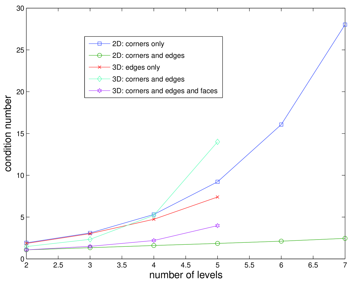
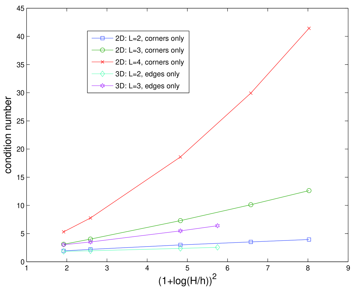
The results in Tables 1 and 2 are displayed in Figure 2 for a fixed value of Hi/Hi1=3H_{i}/H_{i-1}=3. In two dimensions we observe very different behavior depending on the particular form of the coarse space. If only corners are used in 2D, then there is very rapid growth of the condition number with increasing numbers of levels as predicted by the theory. In contrast, if both corners and edges are used in the 2D coarse space, then the condition number appears to vary linearly with LL for the the number of levels considered. Our explanation is that a bound similar to Theorem 25 still applies to the favorable 2D case, though possibly with (much) smaller constants, so the exponential growth of the condition number is no longer apparent. The results in Tables 1 and 2 are also displayed in Figure 3 for fixed numbers of levels. The observed growth of condition numbers for the case of uniform coarsening is consistent with the estimate in (91).

Similar trends are present in 3D, but the beneficial effects of using more enriched coarse spaces are much less pronounced. Interestingly, when comparing the use of edges only (E) with corners and edges (C+E) in the coarse space, the latter does not always lead to smaller numbers of iterations or condition numbers for more than two levels. The fully enriched coarse space (C+E+F), however, does give the best results in terms of iterations and condition numbers. It should be noted that the present 3D theory in Theorem 25 covers only the use of the edges only, and the present theory does not guarantee that the condition number (or even its bound) decrease with increasing the coarse space (Remark 27).

In summary, the numerical examples suggest that better performance, especially in 2D, can be obtained when using a fully enriched coarse space. Doing so does not incur a large computational expense since there is never the need to solve a large coarse problem exactly with the multilevel approach. Finally, we note that a large number of levels is not required to solve very large problems. For example, the number of unknowns in 3D for a 4-level method with a coarsening ratio of Hi/Hi1=10H_{i}/H_{i-1}=10 at all levels is (104)3=1012(10^{4})^{3}=10^{12}.

References

  • [1] S. C. Brenner and Q. He, Lower bounds for three-dimensional nonoverlapping domain decomposition algorithms, Numer. Math., 93 (2003), pp. 445–470.
  • [2] S. C. Brenner and L.-Y. Sung, Lower bounds for nonoverlapping domain decomposition preconditioners in two dimensions, Math. Comp., 69 (2000), pp. 1319–1339.
  • [3]  , BDDC and FETI-DP without matrices or vectors, Comput. Methods Appl. Mech. Engrg., 196 (2007), pp. 1429–1435.
  • [4] C. R. Dohrmann, A preconditioner for substructuring based on constrained energy minimization, SIAM J. Sci. Comput., 25 (2003), pp. 246–258.
  • [5] M. Dryja and O. B. Widlund, Schwarz methods of Neumann-Neumann type for three-dimensional elliptic finite element problems, Comm. Pure Appl. Math., 48 (1995), pp. 121–155.
  • [6] C. Farhat, M. Lesoinne, P. LeTallec, K. Pierson, and D. Rixen, FETI-DP: a dual-primal unified FETI method. I. A faster alternative to the two-level FETI method, Internat. J. Numer. Methods Engrg., 50 (2001), pp. 1523–1544.
  • [7] C. Farhat, M. Lesoinne, and K. Pierson, A scalable dual-primal domain decomposition method, Numer. Linear Algebra Appl., 7 (2000), pp. 687–714. Preconditioning techniques for large sparse matrix problems in industrial applications (Minneapolis, MN, 1999).
  • [8] C. Farhat and F.-X. Roux, A method of finite element tearing and interconnecting and its parallel solution algorithm, Internat. J. Numer. Methods Engrg., 32 (1991), pp. 1205–1227.
  • [9] A. Klawonn and O. B. Widlund, Dual-primal FETI methods for linear elasticity, Comm. Pure Appl. Math., 59 (2006), pp. 1523–1572.
  • [10] J. Li and O. B. Widlund, FETI-DP, BDDC, and block Cholesky methods, Internat. J. Numer. Methods Engrg., 66 (2006), pp. 250–271.
  • [11]  , On the use of inexact subdomain solvers for BDDC algorithms, Comput. Methods Appl. Mech. Engrg., 196 (2007), pp. 1415–1428.
  • [12] J. Mandel, Balancing domain decomposition, Comm. Numer. Methods Engrg., 9 (1993), pp. 233–241.
  • [13] J. Mandel and C. R. Dohrmann, Convergence of a balancing domain decomposition by constraints and energy minimization, Numer. Linear Algebra Appl., 10 (2003), pp. 639–659. Dedicated to the 70th birthday of Ivo Marek.
  • [14] J. Mandel, C. R. Dohrmann, and R. Tezaur, An algebraic theory for primal and dual substructuring methods by constraints, Appl. Numer. Math., 54 (2005), pp. 167–193.
  • [15] J. Mandel and B. Sousedík, Adaptive selection of face coarse degrees of freedom in the BDDC and the FETI-DP iterative substructuring methods, Comput. Methods Appl. Mech. Engrg., 196 (2007), pp. 1389–1399.
  • [16] J. Mandel, B. Sousedík, and C. R. Dohrmann, On multilevel BDDC, Lecture Notes in Computational Science and Engineering, 60 (2007), pp. 287–294. Domain Decomposition Methods in Science and Engineering XVII.
  • [17] B. F. Smith, P. E. Bjørstad, and W. D. Gropp, Domain decomposition, Cambridge University Press, Cambridge, 1996. Parallel multilevel methods for elliptic partial differential equations.
  • [18] A. Toselli and O. Widlund, Domain decomposition methods—algorithms and theory, vol. 34 of Springer Series in Computational Mathematics, Springer-Verlag, Berlin, 2005.
  • [19] X. Tu, Three-level BDDC in three dimensions, SIAM J. Sci. Comput., 29 (2007), pp. 1759–1780.
  • [20]  , Three-level BDDC in two dimensions, Internat. J. Numer. Methods Engrg., 69 (2007), pp. 33–59.