Multiview Equivariance Improves 3D Correspondence Understanding with Minimal Feature Finetuning
Abstract
Vision foundation models, particularly the ViT family, have revolutionized image understanding by providing rich semantic features. However, despite their success in 2D comprehension, their abilities on grasping 3D spatial relationships are still unclear. In this work, we evaluate and enhance the 3D awareness of ViT-based models. We begin by systematically assessing their ability to learn 3D equivariant features, specifically examining the consistency of semantic embeddings across different viewpoints. Our findings indicate that improved 3D equivariance leads to better performance on various downstream tasks, including pose estimation, tracking, and semantic transfer. Building on this insight, we propose a simple yet effective finetuning strategy based on 3D correspondences, which significantly enhances the 3D correspondence understanding of existing vision models. Remarkably, finetuning on a single object for one iteration results in substantial gains.

1 Introduction
Common camera imaging systems struggle to depict the 3D world due to the limitation of capturing only a single perspective at any given moment. In contrast, human perceptual capabilities exhibit a remarkable trait known as view equivariance Köhler (1967); Koffka (2013); Wilson & Farah (2003), allowing us to robustly understand 3D spatial relationships, as seen in tasks ranging from basic object recognition Vetter et al. (1995); DiCarlo & Cox (2007) to more complex processes like mental rotation and simulation Stewart et al. (2022).
Current large vision models, however, are primarily trained on 2D images, owing to the ease of data acquisition and annotation in 2D. Consequently, their performance is typically evaluated on 2D tasks Amir et al. (2021); Hedlin et al. (2023); Tang et al. (2023); Zhang et al. (2023). This raises critical questions: To what extent do these models possess an inherent awareness of 3D structures? How does this awareness impact their performance on image-based 3D vision tasks? And, can we further enhance the 3D awareness of these vision foundation models?
Many image-based 3D scene understanding and content generation tasks depend heavily on large 2D vision models, underscoring the importance of investigating these questions. Existing works have begun to explore this area in task-specific contexts. For example, DietNeRF Jain et al. (2021) finds that CLIP Radford et al. (2021) demonstrates higher feature similarities between views from the same scene than from different scenes, which aids 3D reconstruction. LeRF Kerr et al. (2023) shows that regularizing CLIP with DINO Caron et al. (2021) features improves 3D feature distillation from multiple views. However, these studies are tied to specific tasks such as feature distillation. El Banani et al. (2024) probes the multi-view consistency of ViTs on the NAVI Jampani et al. (2023) and ScanNet Dai et al. (2017) datasets. However, the limited size of these datasets makes it challenging to draw comprehensive conclusions.
To address the first question, how well do vision models understand 3D structures, we present a comprehensive study of the 3D awareness of large 2D vision models. Specifically, we investigate the view equivariance of latent features—i.e., the consistency of multi-view 2D image features representing the same 3D point across different views. Using off-the-shelf multiview correspondences rendered from Objaverse Deitke et al. (2023) (synthetic) and MVImgNet Yu et al. (2023) (real-world), we find that current large vision models do exhibit some degree of view-consistent feature generation, with DINOv2 demonstrating the strongest performance.
To answer the second question, how does this awareness influence performance in image-based 3D vision tasks, we find that the quality of 3D equivariance is strongly correlated with performance on three downstream tasks requiring 3D correspondence understanding: pose estimation, video tracking, and semantic correspondence. Consistent with previous findings Örnek et al. (2023); Tumanyan et al. (2024); Zhang et al. (2023), DINOv2 Oquab et al. (2023) excels in these tasks.
Finally, to address the third question, can we improve the 3D awareness of vision foundation models, we propose a simple yet effective method to enhance the view equivariance of 2D foundation models, thereby significantly improving their 3D correspondence understanding. During training, we randomly select two different views of the same object from Objaverse and sample corresponding pixels. We apply the SmoothAP Brown et al. (2020) loss to enforce feature similarity between these corresponding pixels. This finetuning process, requiring only 10K iterations with LoRA and an additional convolutional layer of a Vision Transformer (ViT), significantly improves the performance of all tested models on 3D tasks. For instance, DINOv2 gains improvements of 9.58 (3cm-3deg in pose estimation), 5.0 (Average Jaccard in tracking), and 5.06 (PCK@0.05 in semantic correspondence). Surprisingly, even finetuning on a single multi-view pair sampled from one object for just one iteration yields notable gains in 3D correspondence understanding. In such cases, DINOv2’s performance improves by 4.85, 3.55, and 3.47 for 3cm-3deg (pose estimation), Average Jaccard (tracking), and PCK@0.05 (semantic correspondence), respectively.
To summarize, our key contributions are: (i) We conduct a comprehensive evaluation of 3D equivariance capabilities in 2D vision foundation models. (ii) We demonstrate that the quality of 3D equivariance is closely tied to performance on three downstream tasks that require 3D correspondence understanding: pose estimation, video tracking, and semantic correspondence. (iii) We propose a simple but effective finetuning method that improves the 3D correspondence understanding of 2D foundation models, leading to marked performance gains across all evaluated tasks.
2 Evaluation of Multiview Feature Equivariance
To assess how effectively current vision transformers capture 3D correspondence understanding, we introduce a 3D equivariance evaluation benchmark focused on the quality of correspondences between 2D points across different views for the same object. Additionally, we present three well-established application tasks that rely on 3D correspondence, demonstrating a strong correlation between the quality of 3D equivariance and downstream task performance. We evaluate five state-of-the-art vision transformers: DINOv2 Oquab et al. (2023), DINOv2-Reg Darcet et al. (2023), MAE He et al. (2022a), CLIP Radford et al. (2021) and DeiT Touvron et al. (2022), extracting their final-layer features with L2 normalization. For DINOv2, we use the base model; results for other variants are provided in the supplementary material.
To evaluate 3D equivariance, we utilize rendered or annotated multiview correspondences from Objaverse Deitke et al. (2023) and MVImgNet Yu et al. (2023), covering both synthetic and real images. For Objaverse, we randomly select 1,000 objects from the Objaverse repository, rendered across 42 uniformly distributed camera views, producing 42,000 images. Dense correspondences are computed for each object across every unique ordered pair of views, resulting in 1.8 billion correspondence pairs for evaluation. Similarly, 1,000 objects are randomly drawn from MVImgNet, yielding 33.3 million annotated correspondence pairs for evaluation. Since MVImgNet employs COLMAP to reconstruct 3D points, it provides sparser correspondences compared to Objaverse.

Metric and Results
We propose the Average Pixel Error% (APE), a metric that quantifies the average distance between predicted and ground-truth pixel correspondences, normalized by the length of the shortest image edge. The predicted correspondence is determined by identifying the nearest neighbor in the second view, given a reference point feature in the first view. APE for Objaverse is shown in Figure 3, where APE is plotted on the x-axis, meaning lower values (towards the left) indicate better performance. APE and PCDP for MVImgNet are plotted on Figure 5’s y-axis with hollow circle and striped bar representing the evaluted pretrained models (fine-tuning results will be discussed later). Percentage of Correct Dense Points% (PCDP) is a metric designed to evaluate dense correspondences, similar to Percentage of Correct Keypoints% (PCK). It is reported at various thresholds (5%, 10%, and 20% of the shortest image edge). We can see that DINOv2 and its registered version outperform other vision transformers, highlighting DINOv2’s superior capability for 3D equivariance. In Figure 2, we provide feature visualizations using PCA, where DINOv2 again demonstrates the best multiview feature consistency.


2.1 Feature Equivariance Correlates to Certain Task Performances
3D Equivariance itself is not interesting unless it can be used. Below, we will talk about three mature downstream applications that require 3D equivariance capability, and show a correlation between the quality of 3D equivariance and the downstream applications.
2.1.1 Task Definitions
One-Shot Object Pose Estimation
In one-shot pose estimation, we assume access to a video sequence or 3D mesh of the target object and aim to estimate its pose in arbitrary environments. During onboarding, we store dense 2D image features from all rendered or annotated views in a database. At inference, we compute correspondences between the input image and the stored features to match 2D keypoints in the image to their 3D counterparts. Pose estimation from these 2D-3D correspondences is achieved using RANSAC Fischler & Bolles (1981) PnP (Perspective-n-Point). Points are uniformly sampled using stratified sampling (stride 4) on resized images. RANSAC PnP runs for 10,000 iterations with a threshold of 8.
We evaluate on the OnePose-LowTexture and YCB-Video datasets. OnePose-LowTexture He et al. (2022b) includes 40 low-textured household items captured in two videos: one for reference and one for testing, simulating a one-shot scenario. We evaluate on every 10 frames in the video. Following He et al. (2022b), pose accuracy is evaluated using 1cm-1deg, 3cm-3deg, and 5cm-5deg thresholds. The YCB-Video dataset Xiang et al. (2017) comprises 21 objects and 92 RGB-D video sequences with pose annotations and CAD models for one-shot generalization. A database is created by rendering objects from 96 icospherical viewpoints. We report Average Recall (AR) for Visible Surface Discrepancy (VSD), Maximum Symmetry-Aware Surface Distance (MSSD), and Maximum Symmetry-Aware Projection Distance (MSPD) following Hodaň et al. (2020).
Video Tracking
For video tracking, given the reference frame, we identify corresponding points in other frames by computing cosine similarities between the dense features of the target object. To improve robustness and accuracy, we follow the process in DINO-Tracker Tumanyan et al. (2024), which applies a softmax operation within the neighborhood of the location with highest similarity.
We evaluate the models on the TAP-Vid-DAVIS Doersch et al. (2022) dataset, a benchmark designed for testing video tracking in complex, real-world scenarios. Performance is measured using commonly applied metrics Tumanyan et al. (2024), including the Average Jaccard Index (AJ), Position Accuracy (), and Occlusion Accuracy (OA).
Semantic Correspondence
In the semantic correspondence task, we utilize feature correspondences to establish precise keypoint matches between images captured from different instances from the same category. Following the method in Zhang et al. (2023), for a given reference keypoint, we identify the best match by selecting the location with the highest cosine feature similarity.
We use the PF-PASCAL Ham et al. (2017) dataset as our evaluation benchmark. This dataset typically consists of image pairs taken from the same viewpoint, but we additionally report the result by shuffling the image pairs to include different viewpoints, thereby increasing the challenge. We follow standard practice to use PCK@0.05, PCK@0.10, and PCK@0.15 as evaluation metrics.
The pipelines for all three tasks are illustrated in the figures provided in the supplementary material.
2.1.2 On the Choice of Three Tasks
Correspondence estimation is a fundamental component of 3D vision understanding, underlying key tasks such as epipolar geometry, stereo vision for 3D reconstruction, and optical flow or tracking to describe the motion of a perceived 3D world. Stereo cameras, and even human perception, rely on disparity maps—effectively, correspondences between projected 3D parts to understand depth and spatial relationships.
The three tasks we evaluated—pose estimation, video tracking, and semantic correspondence—are intentionally selected to cover diverse aspects of correspondence estimation, ranging from simpler to more complex scenarios: 1. Pose Estimation examines correspondences within the same instance under rigid transformations (); 2. Video Tracking extends this to correspondences for the same instance under potential non-rigid or articulated transformations, such as humans or animals in motion; 3. Semantic Correspondence requires correspondences across different instances with similar semantics, often under arbitrary viewpoint changes. An qualitative illustration of these correspondence types is shown in Figure 4.

2.1.3 Results and Findings
Quantitative results are presented in Figure 3, where the y-axis in each graph shows the performance of the vision models. DINOv2 consistently outperforms all other models across all three tasks, in alignment with the rankings for 3D equivariance on the x-axis. There is a clear correlation between the quality of 3D equivariance and performance on the downstream tasks: methods with lower APE tend to perform better across all tasks, clustering towards the top-left of the graphs.
3 Feature Finetuning with Multiview Equivariance
Given the correlation between the multiview equivariance of network features and task performances, we naturally come up with a question: Can we finetune the networks on feature equivariance to improve their 3D correspondence understanding and achieve better task performances?
Finetuning method
The high-level intuition of improving the multiview equivariance of the network features is to enforce the similarity between features of corresponding pixels in 3D space. We experiment with multiple strategies including different training objectives and network architectures.
For the training loss, rather than employing a conventional contrastive loss, we opted for the SmoothAP Brown et al. (2020) loss, which demonstrated superior performance. While contrastive loss can help align the features of corresponding pixels, it relies on a predefined fixed margin for positive and negative samples, which is ad hoc and often suboptimal. In contrast, SmoothAP optimizes a ranking loss directly, leading to an improved average precision for feature retrieval between corresponding pixels. We also experimented with the differentiable Procrustes alignment loss Li et al. (2022), but it did not outperform. Detailed ablation results are given in Section 4.3.
In terms of architecture, we apply LoRA in the last four blocks to finetune large foundation models, we introduced a single convolutional layer with a kernel size of 3 and a stride of 1. The motivation behind this addition is rooted in the observation that ViT-family models process image tokens as patches, resulting in much lower-resolution feature maps (e.g., 14x smaller in DINOv2). The standard approach to obtain high-resolution per-pixel features is to apply linear interpolation. Consequently, it is beneficial to explicitly exchange information between neighboring patches before interpolation to achieve more accurate results. More ablation results are given in Section 4.1.
During training, we randomly select two views of the same object from a 10K subset of Objaverse at each iteration and sample corresponding pixels. The model is trained for 10K iterations using the AdamW optimizer with a learning rate of 1e-5 and weight decay of 1e-4. In the supplementary, we show that our finetuning method is robust to the choice of learning rate.


3.1 Improved Feature Equivariance with Generalization
Figure 5 illustrates the performance of various models before and after finetuning. After fine-tuning on Objaverse, all models show improved 3D equivariance on both Objaverse (synthetic) and MVImgNet (real-world). This demonstrates the capacity of vision foundation models to perform sim-to-real transfer, as finetuning on synthetic Objaverse objects results in enhanced performance on the real-world MVImgNet dataset. Additionally, the performance on the two datasets is correlated, with data points roughly aligning along the diagonal, indicating that improvements in synthetic environments translate well to real-world settings. DINOv2 stands out as the best model. We also compare the feature visualizations before and after finetuning in Figure 6, from which we can see that after finetuning the model produces more consistent features with less noise.
3.2 Improved Task Performances


One-shot Object Pose Estimation
Figure 7 shows the performance of pose estimation on the OnePose-LowTex and YCB-Video datasets before and after fine-tuning. As illustrated, all Vision Transformers (ViTs) exhibit noticeable improvements after being fine-tuned on synthetic Objaverse data. For instance, the best-performing model, DINOv2-Reg, improves by 3.46, 6.67, and 6.92 for the 1cm-1deg, 3cm-3deg, and 5cm-5deg thresholds, respectively. Additionally, models that performed weaker before fine-tuning show larger gains. For example, DeiT improves by 4.65, 16.39, and 17.76. Similar trends are observed for the YCB-Video dataset, where models like MAE, initially the weakest, show substantial improvement after fine-tuning.


Video Tracking
Similarly, in the video tracking task, we observe consistent improvements across all ViTs after fine-tuning, as shown in Figure 8. The top-performing model, DINOv2, achieves improvements of 6.45, 5.73, and 2.69 in AJ, , and OA, respectively.
Semantic Correspondence
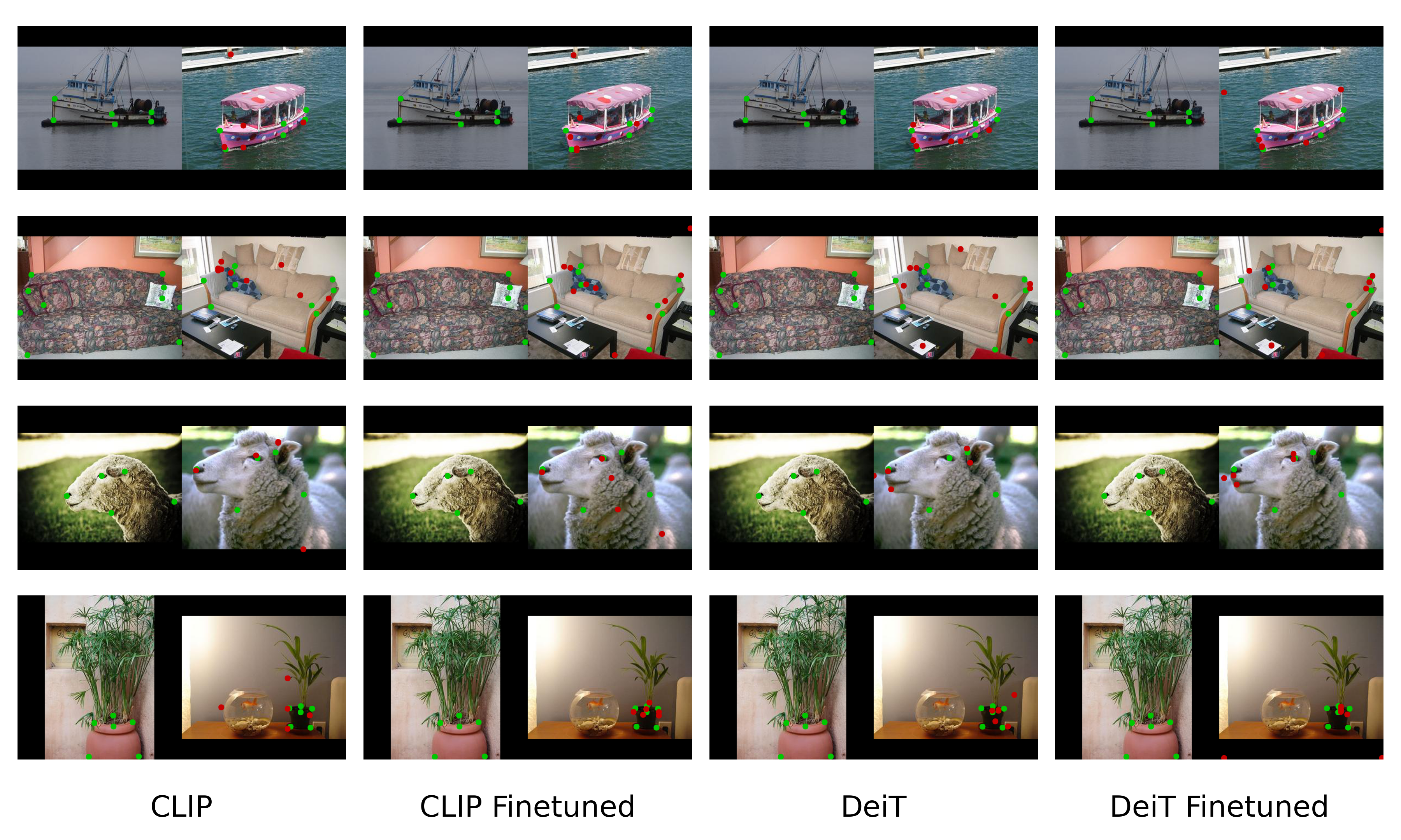
In the semantic correspondence task, shown in Figure 9, DINOv2 exhibits improvements of 5.06, 3.86, and 1.98 for PCK@0.05, PCK@0.10, and PCK@0.15, respectively. Notably, we find that fine-tuned models show enhanced understanding of keypoint semantics across different instances, even from the same viewpoint. This suggests that 3D equivariance contributes to a better understanding of fine-grained semantics, despite not finetuned for that purpose.
3.3 Extremely Few-Shot Finetuning


Training with Only One Object
We plot the performance relative to the number of training objects used, as shown in Figure 10, keeping the total number of iterations fixed at 10K. Surprisingly, fine-tuning on just one object already provides significant performance improvements. Additionally, the object was randomly selected from Objaverse. We tested six different objects, all of which yielded similar results. The results are shown in Figure 11. Notably, even simple shapes like an untextured hemisphere can enhance the 3D correspondence understanding of the ViTs in these tasks.

Convergence Within a Few Iterations
Figure 12 plots the performance of downstream tasks versus the number of training iterations on a single object. Interestingly, our experiments reveal that training with just a single multi-view pair of one object for a single iteration significantly boosts the model’s 3D equivariance, as shown by the sharp improvement at the first elbow of Figure 12. This finding is remarkable, indicating that fine-tuning for 3D correspondence in vision transformers is highly efficient in capturing essential 3D spatial relationships with minimal data. Even with such a minimal training setup, the model effectively learns the desired 3D properties, substantially improving performance across tasks without requiring extensive training or large datasets.
3.4 Finetuning ViT Enhances 3D Tasks in the Wild
A key advantage of theViT features studied here are highly generalizable across diverse datasets and tasks, supporting a even wider range of applications. For example, SparseDFF Wang et al. (2023) uses DINO to aggregate and fine-tune consistent features across views for few-shot transfer manipulation policy learning; LERF Kerr et al. (2023) employs dense DINO features for regularization; and Wild Gaussians Kulhanek et al. (2024) utilizes off-the-shelf DINO features as priors to estimate occlusions and reconstruct 3D scenes in complex settings. To demonstrate the effectiveness of our fine-tuned features, we conducted experiments on Wild Gaussians (W-G) and found that replacing the original features with our fine-tuned DINO features improved novel view synthesis quality in the wild, as shown in Table 1. Additionally, in the supplementary we show that substituting LERF’s DINO regularizer with our fine-tuned version enhances language-embedded field performance, with detailed results and analysis provided therein.
| Mountain | Fountain | Corner | Patio | Spot | Patio-High | |||||||||||||
| PSNR | SSIM | LPIPS | PSNR | SSIM | LPIPS | PSNR | SSIM | LPIPS | PSNR | SSIM | LPIPS | PSNR | SSIM | LPIPS | PSNR | SSIM | LPIPS | |
| W-G | 20.82 | 0.668 | 0.239 | 20.90 | 0.668 | 0.213 | 23.51 | 0.810 | 0.152 | 21.31 | 0.802 | 0.134 | 23.96 | 0.777 | 0.165 | 22.04 | 0.734 | 0.202 |
| Ours | 21.01 | 0.672 | 0.234 | 20.97 | 0.672 | 0.212 | 23.74 | 0.810 | 0.151 | 21.23 | 0.802 | 0.133 | 24.01 | 0.778 | 0.163 | 22.11 | 0.734 | 0.201 |


4 Design Choices for Finetuning
In this section, we ablate and verify the design choices of our finetuning strategy and share some findings. We use the best DINOv2 base model for all our ablations.
4.1 Additional Convolution Layer Head
We append a single convolution layer to the original model architecture and find that gives surprisingly good performance. Adding a single convolutional layer to the finetuning architecture was motivated by the need to improve the resolution and consistency of the dense feature maps produced by Vision Transformer (ViT) models. The typical ViT models process images as low-resolution patches, and while global attention mechanisms facilitate communication between patches, they are not optimized for generating dense per-pixel features during interpolation. By incorporating a convolutional layer with a kernel size of 3 and a stride of 1, we can explicitly exchange information between neighboring patches, allowing the model to generate more accurate and high-resolution feature maps before interpolation. We ablate the number of convolutional layers and table 2 shows that one conv layer gives the best performance.
| ViT models | OnePose-LowTex | TAP-VID-DAVIS | PF-PASCAL (Diff. View) | ||||||
| 1cm-1deg | 3cm-3deg | 5cm-5deg | AJ | OA | PCK0.05 | PCK0.10 | PCK0.15 | ||
| DINOv2-FT (Conv 0) | 11.69 | 53.85 | 72.83 | 44.50 | 60.79 | 84.08 | 44.82 | 57.14 | 65.26 |
| DINOv2-FT (Conv 1) | 13.58 | 58.03 | 77.35 | 46.85 | 63.84 | 84.15 | 47.25 | 60.76 | 67.57 |
| DINOv2-FT (Conv 2) | 13.12 | 56.14 | 75.45 | 47.42 | 63.25 | 84.12 | 46.32 | 58.05 | 64.90 |
| DINOv2-FT (Conv 3) | 12.15 | 53.63 | 74.46 | 46.84 | 62.14 | 82.90 | 41.60 | 53.97 | 60.22 |
4.2 Training Data
MVImgNet v.s. Objaverse
Our results indicate that finetuning on MVImgNet is slightly worse compared to finetuning on Objaverse, likely due to the denser correspondences provided by Objaverse. Both datasets provide a similar object-centric multi-view setup. Although Objaverse is a synthetic dataset and MVImgNet consists of real-world captures, large foundation models tend to be largely agnostic to the distinction between simulated and real images.
Object-centric datasets v.s. scene-centric datasets
An interesting result, as shown in Table 3, is that finetuning on scene-centric datasets (e.g. RealEstate10K Zhou et al. (2018), Spaces Flynn et al. (2019), and LLFF Mildenhall et al. (2019), which contain diverse real-world scenes with complex backgrounds, does not necessarily improve the performance but sometimes make it worse (e.g. PF-PASCAL). This may indicate that 3D objects themselves have already encoded enough 3D spatial reasoning information. And scene-centric dataset does include much more background clutter that may distract the network, leading to less accurate feature representations.
| ViT models | OnePose-LowTex | TAP-VID-DAVIS | PF-PASCAL (Diff. View) | ||||||
| 1cm-1deg | 3cm-3deg | 5cm-5deg | AJ | OA | PCK0.05 | PCK0.10 | PCK0.15 | ||
| DINOv2-FT (Objaverse) | 13.58 | 58.03 | 77.35 | 46.85 | 63.84 | 84.15 | 47.25 | 60.76 | 67.57 |
| DINOv2-FT (MVImgNet) | 13.65 | 56.98 | 74.61 | 41.53 | 58.89 | 82.67 | 45.13 | 57.93 | 65.40 |
| DINOv2-FT (Scene-Centric) | 15.95 | 60.79 | 76.35 | 47.36 | 63.07 | 80.27 | 41.73 | 52.33 | 60.33 |
| ViT models | OnePose-LowTex | TAP-VID-DAVIS | PF-PASCAL (Diff. View) | ||||||
| 1cm-1deg | 3cm-3deg | 5cm-5deg | AJ | OA | PCK0.05 | PCK0.10 | PCK0.15 | ||
| DINOv2-FT (SmoothAP) | 13.58 | 58.03 | 77.35 | 46.85 | 63.84 | 84.15 | 47.25 | 60.76 | 67.57 |
| DINOv2-FT (Contrastive) | 13.28 | 55.57 | 75.68 | 43.79 | 62.20 | 81.84 | 46.70 | 58.08 | 66.21 |
| DINOv2-FT (DiffProc) | 12.92 | 55.00 | 74.86 | 43.60 | 61.32 | 82.74 | 43.89 | 57.22 | 64.66 |
4.3 Loss Functions
We start with naive contrastive loss and found that it does not perform as well. This is because contrastive loss does not directly optimize for the correspondence. In contrast, SmoothAP optimizes a ranking loss directly, leading to an improved average precision for feature retrieval between corresponding pixels. We also experimented with the differentiable Procrustes alignment loss from Li et al. (2022), but it did not outperform SmoothAP. Detailed comparisons are given in Table 4.
5 Related Works
Vision Transformers Dosovitskiy (2020) (ViTs) have made significant strides in image understanding by employing self-attention mechanisms to capture global contextual information, outperforming traditional convolutional neural networks (CNNs) in tasks such as image classification and object detection. However, despite their success in 2D applications, adapting these models to grasp 3D spatial relationships remains a challenging and relatively unexplored area.
There is growing interest in assessing the 3D comprehension of vision models. While some studies have investigated how well generative models capture geometric information from a single image Bhattad et al. (2024); Du et al. (2023); Sarkar et al. (2024), these efforts are generally specific to generative models, limiting their applicability to broader vision tasks. More closely aligned with our work is El Banani et al. (2024), which evaluated the 3D awareness of visual foundation models through task-specific probes and zero-shot inference using frozen features. In contrast, we delve deeper and introduce a simple yet effective method for finetuning 3D awareness in ViTs.
Several researchers have also explored applying large-scale models to 3D tasks. For instance, some approaches utilize features from pre-trained models for tasks such as correspondence matching Zhang et al. (2023); Cheng et al. (2024) and pose estimation Örnek et al. (2023). ImageNet3D Ma et al. (2024) investigates how global tokens from ViT vary across views to aid pose estimation. While their work focuses on view-dependent global features, ours emphasizes dense, pixel-level features invariant to viewpoint changes. Their top-down pose estimation approach classifies poses using pretrained features with a domain-specific linear layer, which limits its applicability across diverse datasets. In contrast, we argue that finding correspondences, or learning equivariant representations, is a more effective strategy for general unseen tasks and datasets.
Recent works, such as FiT Yue et al. (2024) and DVT Yang et al. (2024), attempt to finetune pre-trained features. FiT lifts 2D features into 3D space and then projects them back into 2D to enforce 3D consistency. DVT, on the other hand, implements a denoising process to reduce periodic noise artifacts in images, a method that is orthogonal to our approach. Additionally, DUSt3R Wang et al. (2024) directly predicts 3D coordinates for each 2D pixel, but it lacks a shared consistent feature space and forfeits the rich semantic information provided by large vision models.
6 Conclusion
In this work, we systematically evaluated the 3D awareness of large vision models, with a specific focus on their ability to maintain view equivariance. Our comprehensive study demonstrates that current vision transformers, particularly DINOv2, exhibit strong 3D equivariant properties, which significantly correlate with performance on downstream tasks such as pose estimation, video tracking, and semantic transfer. Building on these insights, we introduced a simple yet effective finetuning method that enhances the 3D correspondence understanding of 2D ViTs. By leveraging multiview correspondences and applying a loss function that enforces feature consistency across views, our approach yields substantial improvements in task performance with minimal computational overhead. Remarkably, even a single iteration of finetuning can lead to notable performance gains.
Our findings highlight the importance of 3D equivariance in vision models and provide a practical path to improving 3D correspondence understanding in existing models. We believe this work opens up new opportunities for enhancing the 3D capabilities of vision transformers. All code and resources will be made publicly available to support further research in this direction.
7 Statements
Ethics Statement. Our method leverages open-sourced simulation data and real data whose data collection process follows strict ethical guidelines. In using these data, we follow the same ethical considerations to protect sensitive information. There is no ethical concerns detected of the proposed method to our knowledge, and we will strive to adhere to ICLR code of conduct for future use of the proposed method.
Reproducibility Statement. We provide extensive details for ease of re-implementation. We strive to ensure our method is reproducible and the findings in this paper are generalizalble. We will release code, results, and scripts for reproduction to promote future research in 3D deep learning.
8 Acknowledgements
Yang You is supported in part by the Outstanding Doctoral Graduates Development Scholarship of Shanghai Jiao Tong University. Congyue Deng, Yang You, and Leonidas Guibas acknowledge support from the Toyota Research Institute University 2.0 Program, ARL grant W911NF-21-2-0104, a Vannevar Bush Faculty Fellowship, and a gift from the Flexiv corporation. Yue Wang acknowledges funding supports from Toyota Research Institute, Dolby, and Google DeepMind. Yue Wang is also supported by a Powell Research Award.
References
- Amir et al. (2021) Shir Amir, Yossi Gandelsman, Shai Bagon, and Tali Dekel. Deep vit features as dense visual descriptors. arXiv preprint arXiv:2112.05814, 2(3):4, 2021.
- Bhattad et al. (2024) Anand Bhattad, Daniel McKee, Derek Hoiem, and David Forsyth. Stylegan knows normal, depth, albedo, and more. Advances in Neural Information Processing Systems, 36, 2024.
- Biederman (1987) Irving Biederman. Recognition-by-components: a theory of human image understanding. Psychological review, 94(2):115, 1987.
- Brown et al. (2020) Andrew Brown, Weidi Xie, Vicky Kalogeiton, and Andrew Zisserman. Smooth-ap: Smoothing the path towards large-scale image retrieval. In European conference on computer vision, pp. 677–694. Springer, 2020.
- Caron et al. (2021) Mathilde Caron, Hugo Touvron, Ishan Misra, Hervé Jégou, Julien Mairal, Piotr Bojanowski, and Armand Joulin. Emerging properties in self-supervised vision transformers. In Proceedings of the IEEE/CVF international conference on computer vision, pp. 9650–9660, 2021.
- Cheng et al. (2024) Xinle Cheng, Congyue Deng, Adam Harley, Yixin Zhu, and Leonidas Guibas. Zero-shot image feature consensus with deep functional maps. arXiv preprint arXiv:2403.12038, 2024.
- Dai et al. (2017) Angela Dai, Angel X Chang, Manolis Savva, Maciej Halber, Thomas Funkhouser, and Matthias Nießner. Scannet: Richly-annotated 3d reconstructions of indoor scenes. In Proceedings of the IEEE conference on computer vision and pattern recognition, pp. 5828–5839, 2017.
- Darcet et al. (2023) Timothée Darcet, Maxime Oquab, Julien Mairal, and Piotr Bojanowski. Vision transformers need registers. arXiv preprint arXiv:2309.16588, 2023.
- Deitke et al. (2023) Matt Deitke, Dustin Schwenk, Jordi Salvador, Luca Weihs, Oscar Michel, Eli VanderBilt, Ludwig Schmidt, Kiana Ehsani, Aniruddha Kembhavi, and Ali Farhadi. Objaverse: A universe of annotated 3d objects. In Proceedings of the IEEE/CVF Conference on Computer Vision and Pattern Recognition, pp. 13142–13153, 2023.
- DiCarlo & Cox (2007) James J DiCarlo and David D Cox. Untangling invariant object recognition. Trends in cognitive sciences, 11(8):333–341, 2007.
- Doersch et al. (2022) Carl Doersch, Ankush Gupta, Larisa Markeeva, Adria Recasens, Lucas Smaira, Yusuf Aytar, Joao Carreira, Andrew Zisserman, and Yi Yang. Tap-vid: A benchmark for tracking any point in a video. Advances in Neural Information Processing Systems, 35:13610–13626, 2022.
- Dosovitskiy (2020) Alexey Dosovitskiy. An image is worth 16x16 words: Transformers for image recognition at scale. arXiv preprint arXiv:2010.11929, 2020.
- Du et al. (2023) Xiaodan Du, Nicholas Kolkin, Greg Shakhnarovich, and Anand Bhattad. Generative models: What do they know? do they know things? let’s find out! arXiv preprint arXiv:2311.17137, 2023.
- El Banani et al. (2024) Mohamed El Banani, Amit Raj, Kevis-Kokitsi Maninis, Abhishek Kar, Yuanzhen Li, Michael Rubinstein, Deqing Sun, Leonidas Guibas, Justin Johnson, and Varun Jampani. Probing the 3d awareness of visual foundation models. In Proceedings of the IEEE/CVF Conference on Computer Vision and Pattern Recognition, pp. 21795–21806, 2024.
- Everingham et al. (2010) Mark Everingham, Luc Van Gool, Christopher KI Williams, John Winn, and Andrew Zisserman. The pascal visual object classes (voc) challenge. International journal of computer vision, 88:303–338, 2010.
- Fischler & Bolles (1981) Martin A Fischler and Robert C Bolles. Random sample consensus: a paradigm for model fitting with applications to image analysis and automated cartography. Communications of the ACM, 24(6):381–395, 1981.
- Flynn et al. (2019) John Flynn, Michael Broxton, Paul Debevec, Matthew DuVall, Graham Fyffe, Ryan Overbeck, Noah Snavely, and Richard Tucker. Deepview: View synthesis with learned gradient descent. In Proceedings of the IEEE/CVF Conference on Computer Vision and Pattern Recognition, pp. 2367–2376, 2019.
- Ham et al. (2017) Bumsub Ham, Minsu Cho, Cordelia Schmid, and Jean Ponce. Proposal flow: Semantic correspondences from object proposals. IEEE transactions on pattern analysis and machine intelligence, 40(7):1711–1725, 2017.
- He et al. (2022a) Kaiming He, Xinlei Chen, Saining Xie, Yanghao Li, Piotr Dollár, and Ross Girshick. Masked autoencoders are scalable vision learners. In Proceedings of the IEEE/CVF conference on computer vision and pattern recognition, pp. 16000–16009, 2022a.
- He et al. (2022b) Xingyi He, Jiaming Sun, Yuang Wang, Di Huang, Hujun Bao, and Xiaowei Zhou. Onepose++: Keypoint-free one-shot object pose estimation without cad models. Advances in Neural Information Processing Systems, 35:35103–35115, 2022b.
- Hedlin et al. (2023) Eric Hedlin, Gopal Sharma, Shweta Mahajan, Hossam Isack, Abhishek Kar, Andrea Tagliasacchi, and Kwang Moo Yi. Unsupervised semantic correspondence using stable diffusion. arXiv preprint arXiv:2305.15581, 2023.
- Hodaň et al. (2020) Tomáš Hodaň, Martin Sundermeyer, Bertram Drost, Yann Labbé, Eric Brachmann, Frank Michel, Carsten Rother, and Jiří Matas. Bop challenge 2020 on 6d object localization. In European Conference on Computer Vision, pp. 577–594. Springer, 2020.
- Jain et al. (2021) Ajay Jain, Matthew Tancik, and Pieter Abbeel. Putting nerf on a diet: Semantically consistent few-shot view synthesis. In Proceedings of the IEEE/CVF International Conference on Computer Vision, pp. 5885–5894, 2021.
- Jampani et al. (2023) Varun Jampani, Kevis-Kokitsi Maninis, Andreas Engelhardt, Arjun Karpur, Karen Truong, Kyle Sargent, Stefan Popov, Andre Araujo, Ricardo Martin-Brualla, Kaushal Patel, Daniel Vlasic, Vittorio Ferrari, Ameesh Makadia, Ce Liu, Yuanzhen Li, and Howard Zhou. Navi: Category-agnostic image collections with high-quality 3d shape and pose annotations. In NeurIPS, 2023. URL https://navidataset.github.io/.
- Karaev et al. (2023) Nikita Karaev, Ignacio Rocco, Benjamin Graham, Natalia Neverova, Andrea Vedaldi, and Christian Rupprecht. Cotracker: It is better to track together. arXiv preprint arXiv:2307.07635, 2023.
- Kerr et al. (2023) Justin Kerr, Chung Min Kim, Ken Goldberg, Angjoo Kanazawa, and Matthew Tancik. Lerf: Language embedded radiance fields. In Proceedings of the IEEE/CVF International Conference on Computer Vision, pp. 19729–19739, 2023.
- Koffka (2013) Kurt Koffka. Principles of Gestalt psychology, volume 44. Routledge, 2013.
- Köhler (1967) Wolfgang Köhler. Gestalt psychology. Psychologische Forschung, 31(1):XVIII–XXX, 1967.
- Kulhanek et al. (2024) Jonas Kulhanek, Songyou Peng, Zuzana Kukelova, Marc Pollefeys, and Torsten Sattler. Wildgaussians: 3d gaussian splatting in the wild. arXiv preprint arXiv:2407.08447, 2024.
- Labbé et al. (2022) Yann Labbé, Lucas Manuelli, Arsalan Mousavian, Stephen Tyree, Stan Birchfield, Jonathan Tremblay, Justin Carpentier, Mathieu Aubry, Dieter Fox, and Josef Sivic. Megapose: 6d pose estimation of novel objects via render & compare. arXiv preprint arXiv:2212.06870, 2022.
- Li et al. (2022) Lei Li, Hongbo Fu, and Maks Ovsjanikov. Wsdesc: Weakly supervised 3d local descriptor learning for point cloud registration. IEEE Transactions on Visualization and Computer Graphics, 29(7):3368–3379, 2022.
- Ma et al. (2024) Wufei Ma, Guanning Zeng, Guofeng Zhang, Qihao Liu, Letian Zhang, Adam Kortylewski, Yaoyao Liu, and Alan Yuille. Imagenet3d: Towards general-purpose object-level 3d understanding. arXiv preprint arXiv:2406.09613, 2024.
- Mildenhall et al. (2019) Ben Mildenhall, Pratul P Srinivasan, Rodrigo Ortiz-Cayon, Nima Khademi Kalantari, Ravi Ramamoorthi, Ren Ng, and Abhishek Kar. Local light field fusion: Practical view synthesis with prescriptive sampling guidelines. ACM Transactions on Graphics (ToG), 38(4):1–14, 2019.
- Oquab et al. (2023) Maxime Oquab, Timothée Darcet, Théo Moutakanni, Huy Vo, Marc Szafraniec, Vasil Khalidov, Pierre Fernandez, Daniel Haziza, Francisco Massa, Alaaeldin El-Nouby, et al. Dinov2: Learning robust visual features without supervision. arXiv preprint arXiv:2304.07193, 2023.
- Örnek et al. (2023) Evin Pınar Örnek, Yann Labbé, Bugra Tekin, Lingni Ma, Cem Keskin, Christian Forster, and Tomas Hodan. Foundpose: Unseen object pose estimation with foundation features. arXiv preprint arXiv:2311.18809, 2023.
- Radenović et al. (2018) Filip Radenović, Ahmet Iscen, Giorgos Tolias, Yannis Avrithis, and Ondřej Chum. Revisiting oxford and paris: Large-scale image retrieval benchmarking. In Proceedings of the IEEE conference on computer vision and pattern recognition, pp. 5706–5715, 2018.
- Radford et al. (2021) Alec Radford, Jong Wook Kim, Chris Hallacy, Aditya Ramesh, Gabriel Goh, Sandhini Agarwal, Girish Sastry, Amanda Askell, Pamela Mishkin, Jack Clark, et al. Learning transferable visual models from natural language supervision. In International conference on machine learning, pp. 8748–8763. PMLR, 2021.
- Sarkar et al. (2024) Ayush Sarkar, Hanlin Mai, Amitabh Mahapatra, Svetlana Lazebnik, David A Forsyth, and Anand Bhattad. Shadows don’t lie and lines can’t bend! generative models don’t know projective geometry… for now. In Proceedings of the IEEE/CVF Conference on Computer Vision and Pattern Recognition, pp. 28140–28149, 2024.
- Silberman et al. (2012) Nathan Silberman, Derek Hoiem, Pushmeet Kohli, and Rob Fergus. Indoor segmentation and support inference from rgbd images. In Computer Vision–ECCV 2012: 12th European Conference on Computer Vision, Florence, Italy, October 7-13, 2012, Proceedings, Part V 12, pp. 746–760. Springer, 2012.
- Stewart et al. (2022) Emma EM Stewart, Frieder T Hartmann, Yaniv Morgenstern, Katherine R Storrs, Guido Maiello, and Roland W Fleming. Mental object rotation based on two-dimensional visual representations. Current Biology, 32(21):R1224–R1225, 2022.
- Tang et al. (2023) Luming Tang, Menglin Jia, Qianqian Wang, Cheng Perng Phoo, and Bharath Hariharan. Emergent correspondence from image diffusion. arXiv preprint arXiv:2306.03881, 2023.
- Touvron et al. (2022) Hugo Touvron, Matthieu Cord, and Hervé Jégou. Deit iii: Revenge of the vit. In European conference on computer vision, pp. 516–533. Springer, 2022.
- Tumanyan et al. (2024) Narek Tumanyan, Assaf Singer, Shai Bagon, and Tali Dekel. Dino-tracker: Taming dino for self-supervised point tracking in a single video. arXiv preprint arXiv:2403.14548, 2024.
- Vetter et al. (1995) Thomas Vetter, Anya Hurlbert, and Tomaso Poggio. View-based models of 3d object recognition: invariance to imaging transformations. Cerebral Cortex, 5(3):261–269, 1995.
- Wang et al. (2023) Qianxu Wang, Haotong Zhang, Congyue Deng, Yang You, Hao Dong, Yixin Zhu, and Leonidas Guibas. Sparsedff: Sparse-view feature distillation for one-shot dexterous manipulation. arXiv preprint arXiv:2310.16838, 2023.
- Wang et al. (2024) Shuzhe Wang, Vincent Leroy, Yohann Cabon, Boris Chidlovskii, and Jerome Revaud. Dust3r: Geometric 3d vision made easy. In Proceedings of the IEEE/CVF Conference on Computer Vision and Pattern Recognition, pp. 20697–20709, 2024.
- Wilson & Farah (2003) Kevin D Wilson and Martha J Farah. When does the visual system use viewpoint-invariant representations during recognition? Cognitive Brain Research, 16(3):399–415, 2003.
- Xiang et al. (2017) Yu Xiang, Tanner Schmidt, Venkatraman Narayanan, and Dieter Fox. Posecnn: A convolutional neural network for 6d object pose estimation in cluttered scenes. arXiv preprint arXiv:1711.00199, 2017.
- Yang et al. (2024) Jiawei Yang, Katie Z Luo, Jiefeng Li, Kilian Q Weinberger, Yonglong Tian, and Yue Wang. Denoising vision transformers. arXiv preprint arXiv:2401.02957, 2024.
- Yu et al. (2023) Xianggang Yu, Mutian Xu, Yidan Zhang, Haolin Liu, Chongjie Ye, Yushuang Wu, Zizheng Yan, Chenming Zhu, Zhangyang Xiong, Tianyou Liang, et al. Mvimgnet: A large-scale dataset of multi-view images. In Proceedings of the IEEE/CVF conference on computer vision and pattern recognition, pp. 9150–9161, 2023.
- Yue et al. (2024) Yuanwen Yue, Anurag Das, Francis Engelmann, Siyu Tang, and Jan Eric Lenssen. Improving 2d feature representations by 3d-aware fine-tuning. arXiv preprint arXiv:2407.20229, 2024.
- Zhang et al. (2023) Junyi Zhang, Charles Herrmann, Junhwa Hur, Luisa Polania Cabrera, Varun Jampani, Deqing Sun, and Ming-Hsuan Yang. A tale of two features: Stable diffusion complements dino for zero-shot semantic correspondence. arXiv preprint arXiv:2305.15347, 2023.
- Zhou et al. (2018) Tinghui Zhou, Richard Tucker, John Flynn, Graham Fyffe, and Noah Snavely. Stereo magnification: Learning view synthesis using multiplane images. arXiv preprint arXiv:1805.09817, 2018.
Appendix A Appendix
A.1 Metric and Loss Implementation Details
In this section, we give the detailed mathematical definitions of the evaluation metrics and the loss used in our method.
-
•
Average Pixel Error (APE): Suppose we have objects, each rendered from different views. For a pixel in the first image, the ground-truth corresponding pixel in the second image is determined via back-projection into 3D and re-rendering, excluding occluded points. The evaluated method predicts . APE is computed as:
where are the image width and height.
-
•
Percentage of Correct Dense Points (PCDP): PCDP measures the proportion of predicted points that fall within a normalized threshold of the ground-truth point :
Here is the indicator function and is a threshold (commonly 0.05, 0.1 or 0.15).
-
•
Smooth Average Precision (SmoothAP): SmoothAP is used as the training loss to enforce accurate feature correspondences:
where given a query point , is the positive set containing ground-truth points , is the negative set containing all other points in the second view, and is the sigmoid function, and measures the difference in feature similarity with respect to the query point . Ideally, we want all negative points to have smaller similarities with respect to than all positive ones. In this case, and we get . In training, we optimize the loss: .
A.2 Quantitative Results on Objaverse and MVImgNet
The detailed quantitative results on 3D equivariance of Objaverse and MVImgNet are given in Table 5 and 6.
| Model | PCDP(%) | APE(%) | ||
| 0.05 | 0.1 | 0.2 | ||
| DINOv2 Oquab et al. (2023) | 22.60 | 36.84 | 58.88 | 19.12 |
| finetuned | 30.61 | 43.65 | 61.78 | 17.98 |
| DINOv2-Reg Darcet et al. (2023) | 23.05 | 37.24 | 58.23 | 19.51 |
| finetuned | 22.81 | 36.39 | 57.84 | 19.48 |
| MAE He et al. (2022a) | 16.25 | 30.71 | 55.46 | 20.58 |
| finetuned | 22.57 | 35.94 | 56.93 | 19.88 |
| CLIP Radford et al. (2021) | 17.05 | 33.00 | 57.17 | 20.11 |
| finetuned | 22.54 | 38.01 | 59.71 | 19.17 |
| DeiT Touvron et al. (2022) | 18.07 | 33.89 | 58.05 | 19.72 |
| finetuned | 23.39 | 38.47 | 59.95 | 19.00 |
| Model | PCDP(%) | APE(%) | ||
| 0.05 | 0.1 | 0.2 | ||
| DINOv2 Oquab et al. (2023) | 62.09 | 77.94 | 92.49 | 6.24 |
| finetuned | 71.74 | 83.12 | 93.41 | 4.96 |
| DINOv2-Reg Darcet et al. (2023) | 64.54 | 78.99 | 92.25 | 6.06 |
| finetuned | 64.35 | 78.38 | 92.36 | 5.90 |
| MAE He et al. (2022a) | 59.10 | 75.82 | 91.42 | 6.73 |
| finetuned | 73.76 | 82.58 | 92.75 | 4.76 |
| CLIP Radford et al. (2021) | 46.63 | 63.49 | 80.53 | 11.34 |
| finetuned | 60.23 | 72.78 | 85.69 | 8.42 |
| DeiT Touvron et al. (2022) | 54.63 | 72.36 | 87.64 | 8.34 |
| finetuned | 67.31 | 80.12 | 91.63 | 5.89 |
| Method | OnePose-LowTex | ||
| 1cm-1deg | 3cm-3deg | 5cm-5deg | |
| OnePose++ He et al. (2022b) | 16.8 | 57.7 | 72.1 |
| DUSt3R Wang et al. (2024) | 2.88 | 16.61 | 26.79 |
| FiT Yue et al. (2024) | 1.05 | 9.18 | 16.52 |
| FiT-Reg Yue et al. (2024) | 3.44 | 23.51 | 37.68 |
| DINOv2 Oquab et al. (2023) | 9.43 | 48.45 | 67.45 |
| Finetuned | 13.58 | 58.03 | 77.35 |
| DINOv2-Reg Darcet et al. (2023) | 9.95 | 52.65 | 71.72 |
| Finetuned | 13.41 | 59.32 | 78.64 |
| MAE He et al. (2022a) | 4.41 | 20.76 | 32.27 |
| Finetuned | 10.27 | 39.37 | 52.97 |
| CLIP Radford et al. (2021) | 2.85 | 19.65 | 33.84 |
| Finetuned | 6.72 | 35.63 | 52.94 |
| DeiT Touvron et al. (2022) | 2.55 | 16.85 | 31.67 |
| Finetuned | 7.20 | 33.24 | 49.43 |
| Method | VSD | MSSD | MSPD | AR |
| MegaPose Labbé et al. (2022) | 53.5 | 59.7 | 72.8 | 62.0 |
| DUSt3R Wang et al. (2024) | 11.6 | 11.5 | 15.8 | 13.0 |
| FiT Yue et al. (2024) | 4.4 | 3.2 | 3.4 | 3.7 |
| FiT-Reg Yue et al. (2024) | 10.2 | 9.4 | 11.3 | 10.3 |
| DINOv2 Oquab et al. (2023) | 34.9 | 39.4 | 58.8 | 44.4 |
| Finetuned | 39.9 | 44.4 | 63.9 | 49.4 |
| DINOv2-Reg Darcet et al. (2023) | 34.2 | 37.9 | 55.4 | 42.5 |
| Finetuned | 38.1 | 42.3 | 60.0 | 46.8 |
| MAE He et al. (2022a) | 15.9 | 17.9 | 26.8 | 20.2 |
| Finetuned | 32.2 | 36.8 | 54.0 | 41.0 |
| CLIP Radford et al. (2021) | 17.0 | 19.1 | 31.0 | 22.4 |
| Finetuned | 28.3 | 31.3 | 35.6 | 28.3 |
| DeiT Touvron et al. (2022) | 19.4 | 19.8 | 31.2 | 23.5 |
| Finetuned | 29.4 | 31.1 | 45.6 | 35.4 |
| Method | TAP-VID-DAVIS | ||
| AJ | OA | ||
| Co-Tracker Karaev et al. (2023) | 65.6 | 79.4 | 89.5 |
| DUSt3R Wang et al. (2024) | 13.06 | 22.64 | 77.27 |
| FiT Yue et al. (2024) | 20.45 | 33.46 | 77.27 |
| FiT-Reg | 23.28 | 37.30 | 77.27 |
| DINOv2 Oquab et al. (2023) | 40.40 | 58.11 | 81.46 |
| Finetuned | 46.85 | 63.84 | 84.15 |
| DINOv2-Reg Darcet et al. (2023) | 37.89 | 55.43 | 80.77 |
| Finetuned | 44.91 | 62.23 | 83.85 |
| MAE He et al. (2022a) | 29.99 | 48.16 | 77.27 |
| Finetuned | 36.04 | 54.97 | 77.27 |
| CLIP Radford et al. (2021) | 25.86 | 41.17 | 79.28 |
| Finetuned | 32.13 | 49.31 | 79.09 |
| DeiT Touvron et al. (2022) | 26.80 | 42.06 | 78.45 |
| Finetuned | 32.55 | 48.41 | 78.49 |
| Method | PF-PASCAL | ||
| PCK0.05 | PCK0.10 | PCK0.15 | |
| DUSt3R Wang et al. (2024) | 4.70 | 8.21 | 13.01 |
| FiT Yue et al. (2024) | 13.10 | 23.99 | 33.45 |
| FiT-Reg Yue et al. (2024) | 22.39 | 36.45 | 45.27 |
| DINOv2 Oquab et al. (2023) | 42.18 | 56.90 | 65.59 |
| Ours | 47.24 | 60.76 | 67.57 |
| DINOv2-Reg Darcet et al. (2023) | 38.29 | 53.74 | 61.94 |
| Finetuned | 44.44 | 57.27 | 65.27 |
| MAE He et al. (2022a) | 11.98 | 20.16 | 28.16 |
| Finetuned | 14.45 | 23.79 | 32.56 |
| CLIP Radford et al. (2021) | 13.87 | 24.85 | 35.13 |
| Finetuned | 20.39 | 32.36 | 42.58 |
| DeiT Touvron et al. (2022) | 17.73 | 31.17 | 41.17 |
| Finetuned | 20.24 | 33.29 | 41.62 |
| Method | PF-PASCAL | ||
| PCK0.05 | PCK0.10 | PCK0.15 | |
| DUSt3R Wang et al. (2024) | 2.64 | 8.01 | 15.00 |
| FiT Yue et al. (2024) | 13.96 | 27.42 | 37.39 |
| FiT-Reg Yue et al. (2024) | 26.47 | 45.74 | 55.32 |
| DINOv2 Oquab et al. (2023) | 60.22 | 79.05 | 85.95 |
| Finetuned | 69.16 | 84.94 | 89.82 |
| DINOv2-Reg Darcet et al. (2023) | 52.86 | 71.93 | 80.11 |
| Finetuned | 62.63 | 79.24 | 86.69 |
| MAE He et al. (2022a) | 17.16 | 31.52 | 43.54 |
| Finetuned | 21.26 | 36.16 | 48.52 |
| CLIP Radford et al. (2021) | 17.44 | 31.38 | 41.81 |
| Finetuned | 27.40 | 42.72 | 52.67 |
| DeiT Touvron et al. (2022) | 21.21 | 38.96 | 50.36 |
| Finetuned | 30.18 | 49.69 | 60.34 |
A.3 Quantitative and Qualitative Results on the Three Tasks
We present detailed quantitative results for the three tasks (pose estimation, video tracking, and semantic transfer) in this section. Additionally, we compare our method with DUSt3R Wang et al. (2024), FiT Yue et al. (2024) and FiT-Reg Yue et al. (2024). FiT-Reg is FiT finetuned on DINOv2 with registers Darcet et al. (2023). For pose estimation and tracking, we also provide comparisons with state-of-the-art methods such as OnePose++ He et al. (2022b), MegaPose Labbé et al. (2022), and Co-Tracker Karaev et al. (2023), which are specifically trained on these tasks. The results are summarized in Tables 7, 8, 9, 10, and 11.
Our experiments reveal that although FiT aims for 3D consistency, it significantly disrupts the semantics of certain parts, as shown in Figure 13. While this semantic disruption may be acceptable for FiT’s original tasks like semantic segmentation and depth estimation—where an additional linear head can correct these issues—it becomes problematic for our tasks that require 3D-consistent, dense, pixel-level features. We hypothesize that FiT’s poor performance stems from its naive approach to learning 3D consistency through an explicit 3D Gaussian field. When outliers or noise are present, the simple mean square error causes feature representations to shift toward these outliers.


A.4 Quantitative Results for Other Variants of DINOv2
In addition to evaluating the DINOv2 base model, we tested our finetuning method on other variants, including small, large, and giant. Our method consistently yields improvements across almost all metrics for these model variants. The full results are presented in Table 12.
| ViT models | OnePose-LowTex | TAP-VID-DAVIS | PF-PASCAL (Diff. View) | ||||||
| 1cm-1deg | 3cm-3deg | 5cm-5deg | AJ | OA | PCK0.05 | PCK0.10 | PCK0.15 | ||
| DINOv2-S | 8.14 | 45.77 | 65.79 | 37.56 | 55.04 | 80.54 | 39.02 | 53.26 | 61.49 |
| Finetuned | 12.85 | 56.17 | 74.27 | 45.17 | 61.35 | 83.14 | 41.02 | 53.78 | 60.95 |
| DINOv2-L | 10.83 | 51.68 | 70.01 | 42.56 | 59.88 | 83.29 | 44.22 | 57.92 | 65.85 |
| Finetuned | 13.86 | 58.79 | 77.46 | 49.10 | 65.00 | 85.42 | 51.66 | 62.96 | 70.48 |
| DINOv2-G | 13.58 | 58.73 | 76.27 | 44.79 | 61.01 | 85.27 | 44.57 | 57.63 | 65.76 |
| Finetuned | 14.58 | 60.08 | 78.48 | 50.77 | 66.00 | 85.82 | 50.89 | 61.98 | 68.44 |
| DINOv2-S-reg | 10.25 | 49.04 | 68.83 | 34.61 | 52.21 | 79.35 | 31.30 | 45.47 | 54.73 |
| Finetuned | 12.25 | 56.69 | 75.66 | 40.53 | 58.50 | 81.14 | 38.78 | 52.08 | 59.26 |
| DINOv2-L-reg | 10.89 | 51.17 | 69.99 | 39.47 | 56.69 | 82.26 | 41.26 | 56.24 | 63.38 |
| Finetuned | 14.00 | 58.58 | 77.12 | 46.43 | 63.20 | 84.43 | 48.03 | 60.17 | 67.13 |
| DINOv2-G-reg | 11.14 | 53.84 | 72.28 | 41.39 | 58.62 | 83.09 | 40.94 | 53.84 | 61.87 |
| Finetuned | 14.24 | 59.88 | 79.19 | 47.93 | 64.43 | 85.38 | 47.36 | 59.20 | 66.55 |
A.5 Results for Other Foundation Models with Different Architectures.
In addition to ViT, we apply our method to other architectures like ConvNeXt and find that we can consistently improve its performance on downstream tasks as well as shown in Table 13. However, we’ve also observed that ConvNeXt features are not as good as those of modern ViTs. Nonetheless, we do expect and observe improvements in non-ViT based methods like ConvNeXt. This finding is particularly interesting as it teaches us a valuable lesson: with relatively simple 3D fine-tuning, we can achieve even better 3D features than those obtained through pretraining on a vast set of unstructured 2D images.
| OnePose-LowTex | TAP-VID-DAVIS | PF-PASCAL (Diff. View) | |||||||
| 1cm-1deg | 3cm-3deg | 5cm-5deg | AJ | OA | PCK0.05 | PCK0.10 | PCK0.15 | ||
| ConvNext-small | 3.25 | 13.46 | 21.39 | 15.98 | 26.08 | 74.72 | 10.32 | 16.30 | 22.17 |
| small-finetuned | 5.28 | 19.98 | 28.23 | 16.70 | 26.56 | 74.54 | 11.61 | 19.38 | 25.56 |
| ConvNext-base | 5.10 | 22.22 | 34.81 | 17.57 | 28.21 | 72.47 | 13.62 | 21.03 | 27.81 |
| base-finetuned | 8.05 | 32.69 | 46.41 | 18.53 | 28.48 | 71.24 | 15.64 | 25.37 | 32.13 |
| ConvNext-large | 4.71 | 25.33 | 36.48 | 19.43 | 30.24 | 73.71 | 11.05 | 17.57 | 24.19 |
| large-finetuned | 7.21 | 30.68 | 44.47 | 19.45 | 30.68 | 74.33 | 14.56 | 24.04 | 31.57 |
A.6 Results on Other Semantic-Related Tasks
Here, we report results on other semantic-related tasks less focused on 3D understanding. As shown in Table 14, our finetuning method performs on par or slightly worse compared to baseline models in these tasks. We recon that these tasks do not benefit as much from the dense 3D equivariant features our method emphasizes, but rather from coarse, object-level global features. For instance, in tasks where a plane or side of a box should share the same semantic mask and depth, pixel-level dense features are unnecessary to achieve satisfactory results. Future work can be explored to enhance object-level global feature representation.
Instance Recognition
The objective for this task is to identify and differentiate individual object instances within a scene, even when multiple objects belong to the same class (e.g., recognizing distinct cars in a street scene). This task was evaluated using the Paris-H(ard) Radenović et al. (2018) dataset, with performance measured by mean Average Precision (mAP), which captures the precision-recall trade-off. Two probe training configurations were explored: one utilizing only the class token (Cls) and another concatenating patch tokens with the class token (Cls+Patch). Our fine-tuned model demonstrated performance on par with the DINOv2 baseline, achieving mAP scores of 76.23 for Cls and 75.43 for Cls+Patch.
Semantic Segmentation
This task involves assigning a semantic label to each pixel in an image, thereby grouping regions based on their object class, without distinguishing between individual instances of the same class. The VOC2012 Everingham et al. (2010) dataset was used to evaluate this task, with performance metrics including mean Intersection over Union (mIoU) and mean Accuracy (mAcc). These metrics assess the overlap between predicted segmentation and ground truth, as well as pixel-wise classification accuracy. Our fine-tuned model achieved an mIoU of 82.65 and mAcc of 90.21, performing slightly below but comparable to DINOv2.
Depth Estimation
This task aims to predict the distance to each pixel in an image, effectively generating a depth map that represents the 3D structure of the scene. This task is critical for applications requiring spatial understanding, such as indoor navigation and scene reconstruction. We used the NYUv2 Silberman et al. (2012) dataset for evaluation, employing the accuracy and absolute relative error (abs rel) metrics to assess depth prediction performance. Our fine-tuned model achieved a score of 85.48 and an abs rel of 0.1299, slightly underperforming but comparable to the DINOv2 baseline.
| Model | Paris-H Inst. Recognition | VOC2012 Segmentation | NYUv2 Depth Estimation | |||
| Cls | Cls+Patch | mIoU | mAcc | abs rel | ||
| DINOv2 Oquab et al. (2023) | 75.92 | 73.69 | 83.60 | 90.82 | 86.88 | 0.1238 |
| Finetuned | 76.23 | 75.43 | 82.65 | 90.21 | 85.48 | 0.1299 |
| ViT models | OnePose-LowTex | TAP-VID-DAVIS | PF-PASCAL (Diff. View) | ||||||
| 1cm-1deg | 3cm-3deg | 5cm-5deg | AJ | OA | PCK0.05 | PCK0.10 | PCK0.15 | ||
| DINOv2-FT (LR 1e-6) | 11.86 | 55.03 | 73.12 | 44.79 | 62.56 | 83.17 | 47.34 | 60.10 | 68.23 |
| DINOv2-FT (LR 3e-6) | 13.05 | 57.45 | 75.89 | 45.93 | 63.32 | 83.73 | 47.20 | 60.50 | 67.21 |
| DINOv2-FT (LR 1e-5) | 13.58 | 58.03 | 77.35 | 46.85 | 63.84 | 84.15 | 47.25 | 60.76 | 67.57 |
| DINOv2-FT (LR 3e-5) | 13.15 | 58.33 | 77.49 | 46.70 | 63.45 | 83.35 | 45.70 | 57.96 | 65.99 |
A.7 More results on LERF
In addition to the Wild-Gaussians experiment in our main paper, we visualize LERF 3D features after replacing its DINO regularizer with our fine-tuned version in Figure 14. When given the text query ”plate”, LERF with our fine-tuned DINO produced a better relevancy map than the original. Our relevancy map localizes of the plate region better and reduces noise in irrelevant areas such as cookies. These experiments demonstrate that our 3D fine-tuning produces better general-purpose features that enhance various applications.

A.8 More Ablation Study Analysis
A.8.1 Ablations on Multi-Layer Feature Fusion
In addition to extracting features solely from the last layer (11th), we experiment with two different variations: concatenating the features from the last 4 layers and concatenating features from the 2nd, 5th, 8th, and 11th layers. The results are presented in the Table 16. We find that fusing features from different layers does improve the instance-level correspondence a little bit but greatly harms semantic correspondences in tracking and semantic transfer. This indicates that features from earlier layers focus more on instance-level details, while the final layer captures more semantic information.
| OnePose-LowTex | TAP-VID-DAVIS | PF-PASCAL (Diff. View) | |||||||
| 1cm-1deg | 3cm-3deg | 5cm-5deg | AJ | OA | PCK0.05 | PCK0.10 | PCK0.15 | ||
| Layer 11 | 13.58 | 58.03 | 77.35 | 46.85 | 63.84 | 84.15 | 47.24 | 60.76 | 67.57 |
| Layer 2,5,8,11 | 15.34 | 59.56 | 76.81 | 39.67 | 56.74 | 76.29 | 39.84 | 53.05 | 60.15 |
| Layer 8,9,10,11 | 14.24 | 60.35 | 79.27 | 41.25 | 56.56 | 80.15 | 44.99 | 57.73 | 64.48 |
A.8.2 Ablations on Learning Rate
Our finetuning method is insensitive to the choice of learning rate, and it can work within a reasonable range of learning rates, as shown in Table 15.
A.8.3 Qualitative Results on Number of Convolution Layers
Upon analyzing the effect of additional convolutional layers, we find that while one additional convolutional layer significantly improves the performance, adding two or three layers introduces noise into the features. This noise likely arises from the increased parameter freedom, which can overfit to local patterns and reduce the consistency of dense pixel-wise features, as shown in Figure 15. It clearly show that the additional layers produce less coherent features, leading to a degradation in downstream task performance.

A.9 Other Findings and Discussions
Why Untextured Symmetric Hemisphere can Enhance 3D Understanding?
Unlike a perfect sphere, the hemisphere we used is not completely symmetric and provides information about edges and viewpoint orientation. Our visualization of the learned embeddings in Figure 16 shows that after fine-tuning on the hemisphere, the network achieves better edge correspondences and can differentiate between inward and outward views. Even though the object lacks texture, the shadows and edge features provide sufficient cues for the ViT features to develop 3D understanding.
Similarly, in cognitive science, scientists have discovered that the human brain excels at inferring 3D structure. Biederman’s Recognition-by-Components (RBC) theory Biederman (1987) suggests that humans recognize objects through simple 3D primitives called geons (geometrical ions)—basic shapes such as cubes, cylinders, and cones.

Training without Background Enhances Background-invariance
Interestingly, we observed that finetuning on object-centric datasets without backgrounds enhanced the foundation model’s background invariance. Specifically, when comparing an object on a black background (i.e., no background) with the same object on a natural background from the same viewpoint, the finetuned model demonstrated superior feature consistency across corresponding pixels. We quantitatively validated this finding using pairs of images from a random 1K subset from the MSCOCO val dataset. For each annotated object, one image crop was masked while the other was unmasked. We measured the number of inliers by counting mutual nearest neighbors in the feature space that were within 1 pixel of the ground truth. The results confirmed that our finetuned model significantly improved feature consistency across these variations.
| Method | #Inliers |
| DINOv2 Oquab et al. (2023) | 99 |
| Finetuned | 159 |
| DINOv2-RegDarcet et al. (2023) | 76 |
| Finetuned | 148 |
| MAE He et al. (2022a) | 97 |
| Finetuned | 196 |
| CLIP Radford et al. (2021) | 18 |
| Finetuned | 61 |
| DeiT Touvron et al. (2022) | 25 |
| Finetuned | 81 |

A.10 Pipeline Visualization for Downstream Applications
Figures 18, 19, 20, and 21 illustrate the detailed pipelines for various downstream tasks. Note that for pose estimation, tracking, and semantic transfer, no linear fine-tuning is applied. These tasks exclusively assess the quality of the pretrained features from the ViT.


A.11 Qualitative Results for Pose Estimation/Tracking/Semantic Transfer
In this section, we provide qualitative comparisons on various downstream tasks. The results for pose estimation, tracking, and semantic correspondence are shown in Figures 22, 23 and 24, respectively. Since DINOv2-Reg exhibits performance highly similar to DINOv2, we omit its qualitative results.