Mutual coherent structures for heat and angular momentum transport
in turbulent Taylor-Couette flows

X.-Y. Leng J.-Q. Zhong jinqiang@tongji.edu.cn School of Physics Science and Engineering,
Tongji University, 200092 Shanghai, China

Abstract

In this study we report numerical results of turbulent transport of heat $Nu$ and angular momentum $\nu_{t}/\nu$ in Taylor-Couette (TC) flows subjected to a radial temperature gradient. Direct numerical simulations are performed in a TC cell with a radius ratio $\eta=0.5$ and an aspect ratio $\Gamma=8$ for two Rayleigh numbers ( $Ra=10^{5}$ , $10^{6}$ ) and two Prandtl numbers ( $Pr=0.7$ , $4.38$ ), while the Reynolds number $Re$ varies in the range of $0\leq Re\leq 15000$ . With increasing $Re$ , the flows undergo two distinct transitions: the first transition being from the convection-dominated regime to the transitional regime, with the large-scale meridional circulation evolving into spiral vortices; the second transition occurring in the rotation-dominated regime when Taylor vortices turn from a weakly non-linear state into a turbulent state. In particular, when the flows are governed by turbulent Taylor vortices, we find that both transport processes exhibit power-law scaling: $Nu\sim Re^{0.619\pm 0.015}$ for $Pr=4.38$ , $Nu\sim Re^{0.590\pm 0.025}$ for $Pr=0.7$ and $\nu_{t}/\nu\sim Re^{0.588\pm 0.036}$ for both $Pr$ . These scaling exponents suggest an analogous mechanism for the radial transport of heat and angular momentum, which is further evidenced by the fact that the ratio of turbulent viscosity to diffusivity is independent of $Re$ . To illustrate the underlying mechanism of turbulent transport, we extract the coherent structures by analyzing the spatial distributions of heat and momentum flux densities. Our results reveal mutual turbulent structures through which both heat and angular momentum are transported efficiently.

I Introduction

Turbulent transport processes of heat, mass and momentum are the central aspects in studying turbulence, owing to their close relations to various natural flows [1, 2, 3, 4, 5]. To understand the mechanism of turbulent transport is a challenging task in fluid physics and crucial for the related applications. Taylor-Couette (TC) flow, a fluid layer driven by two concentrically rotating cylinders, is of fundamental interest in many perspectives [6, 4], for example, in probing the angular momentum transport in accretion disks [7, 8, 9]. It is also relevant to various applications in industry such as drag reduction [10, 11] and solidification [12, 13].

In TC flows, the toroidal motion of Taylor vortex (TV) may enhance the mixing and transport efficiency. Hence TC reactors are extensively applied to chemical, food and biology processes [14, 15, 16]. In these applications, a heated or cooled cylinder is inevitable. It is thus desirable to investigate the flow structures and transport properties in the TC systems subjected to a radial temperature gradient. For modest Reynolds number ( $Re$ ), studies of flow regimes, instabilities and pattern formations in such TC systems have attracted a lot of attention, including experiments [17, 18, 19, 20, 21, 22], stability analyses [23, 24, 25, 26] and numerical simulations [27, 28, 29, 30]. However, in turbulent TC flows, much less effort has been made to investigate the complex problem of the turbulent transport processes, which are supposed to be more relevant to most applications in geophysical and industrial flows [8, 9, 10]. To better understand the relationships between the scalar and momentum transport in high- $Re$ regime, it is crucial to predict the interior structures and states of the flows. Furthermore, determination of the scaling laws of heat and momentum transport is vital to extrapolate the existing results from laboratories to large-scale geo- and astrophysical flows. It remains a challenging question to date whether the scalar and momentum transport by TC flows share similar scaling behaviors in the turbulent regime [31, 32, 33].

Coherent structures play an important role in turbulent transport processes [3]. In turbulent TC flows, the momentum transport is implemented by the coherent structures in forms of turbulent TVs and turbulent plumes between adjacent TVs [34, 35, 36]. The meridional advection of TVs sweeps the radial and axial boundaries simultaneously, potentially providing a similar transport mechanism in both directions. Indeed, in recent simulations [33], we find that when an axial temperature gradient is applied in turbulent TC flows, the axial heat-transport scaling is analogous to that of the radial transport of angular momentum [33]. This result confirms the existence of analogy between the axial dispersion of a passive scalar and the radial transport of momentum [31, 32]. In the scenario that a radial temperature difference is applied in TC systems, both heat and angular momentum can be transported radially. In this system, how the large-scale structures, such as TVs, affect the turbulent transport processes is a natural question of great interest.

In this study, we utilize the paradigmatic model of TC systems consisting of a heating (cooling) inner (outer) cylinder with two adiabatic endwalls. We consider the radial transport processes of angular momentum and heat in a high-Reynolds-number regime. The results suggest that, in the regime of turbulent TVs, the radial transport of heat and angular momentum possess similar scaling relationships. Furthermore, by extracting fluid domains of high flux densities, we demonstrate that the heat and momentum transport are manipulated mainly by similar turbulent structures.

II Numerical simulations

II.1 Physical model

We investigate the three-dimensional flow of an incompressible viscous fluid contained between two concentric cylinders of radii $r_{1}$ , $r_{2}$ and height $h$ . The inner wall is rotating about $\mathit{z}$ axis $(e_{z})$ with angular velocity $\omega_{1}$ , while the outer one is set to be fixed. A radial temperature difference $\Delta$ is imposed on the cylinders with the hot inner ( $t_{1}$ ) and cold outer ( $t_{2}$ ) walls. The fluid properties including kinematic viscosity $\nu$ , thermal expansion coefficient $\beta$ and thermal diffusivity $\kappa$ are assumed to be constant. The governing parameters are the Rayleigh number $\mathit{Ra}=\beta{g}\Delta{d}^{3}/{(\nu\kappa)}$ , the Prandtl number $\mathit{Pr}=\nu/\kappa$ and the Reynolds number $Re=\omega_{1}r_{1}d/\nu$ respectively, where $d=r_{2}-r_{1}$ is the gap width and $g$ is the gravitational acceleration. The Richardson number $\mathit{Ri}=Ra/Pr/Re^{2}$ , defined as the ratio of the free fall velocity to the inner-wall velocity, is adopted here to measure the relative strength between thermal convection and TC flow. Two important geometrical parameters entering into the problem are the aspect ratio $\Gamma=h/d$ and the radius ratio $\eta=r_{1}/r_{2}$ . The gap width $d$ , imposed temperature difference $\Delta$ and inner-wall velocity $u_{1}=\omega_{1}r_{1}$ are introduced as the length, temperature and velocity scales. Therefore, within the Boussinesq approximation, the dimensionless Navier-Stokes equations are

\frac{\partial\textbf{U}}{\partial{\tau}}+({\textbf{U}}\cdot\nabla){\textbf{U}}=-\nabla{p}+{\frac{1}{Re}}{\nabla}^{2}\textbf{U}+RiT{\mathit{e_{z}}},\qquad\nabla\cdot{\textbf{U}}=0,

(1)

\frac{\partial{T}}{\partial{\tau}}+({\textbf{U}}\cdot\nabla){T}=\frac{1}{{RePr}}{\nabla}^{2}{T},

(2)

where $\mathit{\tau}$ , $\mathit{p}$ and $\mathit{T}$ are, correspondingly, time, pressure and temperature. And U ( $\mathit{U_{r}}$ , $\mathit{U_{\theta}}$ , $\mathit{U_{z}}$ ) are the components of velocity in radial, azimuthal and axial directions for cylindrical coordinates ( $\mathit{R}$ , $\mathit{\Theta}$ , $\mathit{Z}$ ) respectively. The lower case letters $t$ , u ( $\mathit{u_{r}}$ , $\mathit{u_{\theta}}$ , $\mathit{u_{z}}$ ) and ( $\mathit{r}$ , $\mathit{\theta}$ , $\mathit{z}$ ) denote the dimensional temperature, velocity and coordinates. The dimensionless fluid angular velocity is $\omega$ . It is demonstrated in Appendix A that the effect of centrifugal buoyancy [26, 28] does not change the main results and is thus neglected. The inner and outer cylinders are maintained at fixed temperatures $T_{1}=1$ and $T_{2}=0$ respectively, while endwalls are set to be thermally insulating. No-slip boundaries are applied for velocities at all walls. We use a wide gap with the radius ratio $\eta=r_{1}/r_{2}=0.5$ , and the aspect ratio is $\Gamma=h/d=8$ . This small- $\eta$ system has been discussed widely by numerical simulations [37] and experiments [38, 35].

Heat and angular momentum are two important transport quantities in the present system. In general, the global heat and angular momentum transport are expressed by $Nu$ [39] and $Nu_{\omega}$ [40] respectively. The Nusselt number is defined as $\mathit{Nu}=a^{-1}({{\mathit{RePr}}\left\langle U_{r}T\right\rangle_{V}-\partial_{r}\left\langle{T}\right\rangle_{V}})$ , where $\left\langle\right\rangle_{V}$ denotes the volume- and time-averaging and the geometry factor $a=2d^{2}/(ln(r_{2}/r_{1})(r_{2}^{2}-r_{1}^{2}))$ is induced by the annular gap (see Appendix B). However, owing to the braking effect of the fixed endwalls, $Nu_{\omega}$ decreases along the radial direction in our system [33]. As introduced in Appendix B, we use the dimensionless effective viscosity ${\nu_{t}}/{\nu}={(2Re_{\tau})^{2}}/{Re}$ to represent the angular momentum transport instead of $Nu_{\omega}$ . Here, $Re_{\tau}=0.5u_{\tau}d/\nu$ is the friction Reynolds number with the friction velocity $u_{\tau}^{2}=-\nu r(\partial\left\langle u_{\theta}/r\right\rangle_{\theta z}/\partial r)$ at the inner wall, where $\left\langle\right\rangle_{\theta z}$ denotes the azimuthal-, axial- and time-averaging.

II.2 Numerical method

The equation system is solved using the finite difference scheme developed in Ref. [41] and modified for the cylindrical coordinate [42, 43, 33]. The numerical scheme is a second-order approximation based on the spatial discretization, which is nearly fully conservative with regard to mass, momentum and kinetic energy. The second-order explicit Adams–Bashforth/backward-differentiation scheme is employed for the time discretization. The viscous terms are treated explicitly, and implicit treatment is applied for the diffusion term. At every time step, two Poisson equations, the projection method equation for pressure and the equation for temperature are solved using fast-Fourier transforms in the azimuthal direction and the cyclic reduction direct solver [44]. Towards the walls, the clustered grid is implemented using the hyperbolic tangent coordinate transformation.

The grid sensitivity studies as well as the main results are listed in Tables 2, 3 and 4 in Appendix A. For each set of $Ra$ , results from previous low- $Re$ convection are used as the initial condition for the following high- $Re$ case. Data from initial transient state are excluded, and data taken over statistically steady state are averaged to determine the heat and angular momentum transport. The time convergence is checked by comparing the time averages over the whole and the last halves of the simulation, and the resulting discrepancy is less than $3\%$ . For the temporal resolution, the chosen time step $\Delta t$ satisfies the Courant-Friedrichs-Lewy (CFL) condition, and the CFL number remains less than 0.5. The total run time for each case (including the initial and the averaging stages) is greater than 200 large eddy turnover time units, and the averaging time is not less than 100 large eddy turnover time units.

III Results and discussions

III.1 Global transport of heat and angular momentum

Refer to caption — Figure 1: (a) Global heat transport $Nu$ as a function of $Re$ for $Pr=0.7$ and $4.38$ . Symbols are defined in panel (b). Solid lines denote the power-law fitting $Nu=\alpha Re^{\gamma}$ with $\gamma=0.619$ for $Pr=4.38$ (blue) and $\gamma=0.590$ for $Pr=0.7$ (red). Vertical dashed lines denote the first transition $Re^{*}_{1}$ . Inset: an expanded view of the compensated plot of $Nu$ as a function of $Re$ . Vertical dotted lines denote the second transition $Re^{*}_{2}$ . Dashed auxiliary lines indicate the values for the prefactor $\alpha=Nu/Re^{\gamma}$ =0.106 with $\gamma=0.619$ (blue) and $\alpha$ =0.068 with $\gamma=0.590$ (red). (b) $Nu$ as a function of $Ri$ .

III.1.1 Radial heat transport

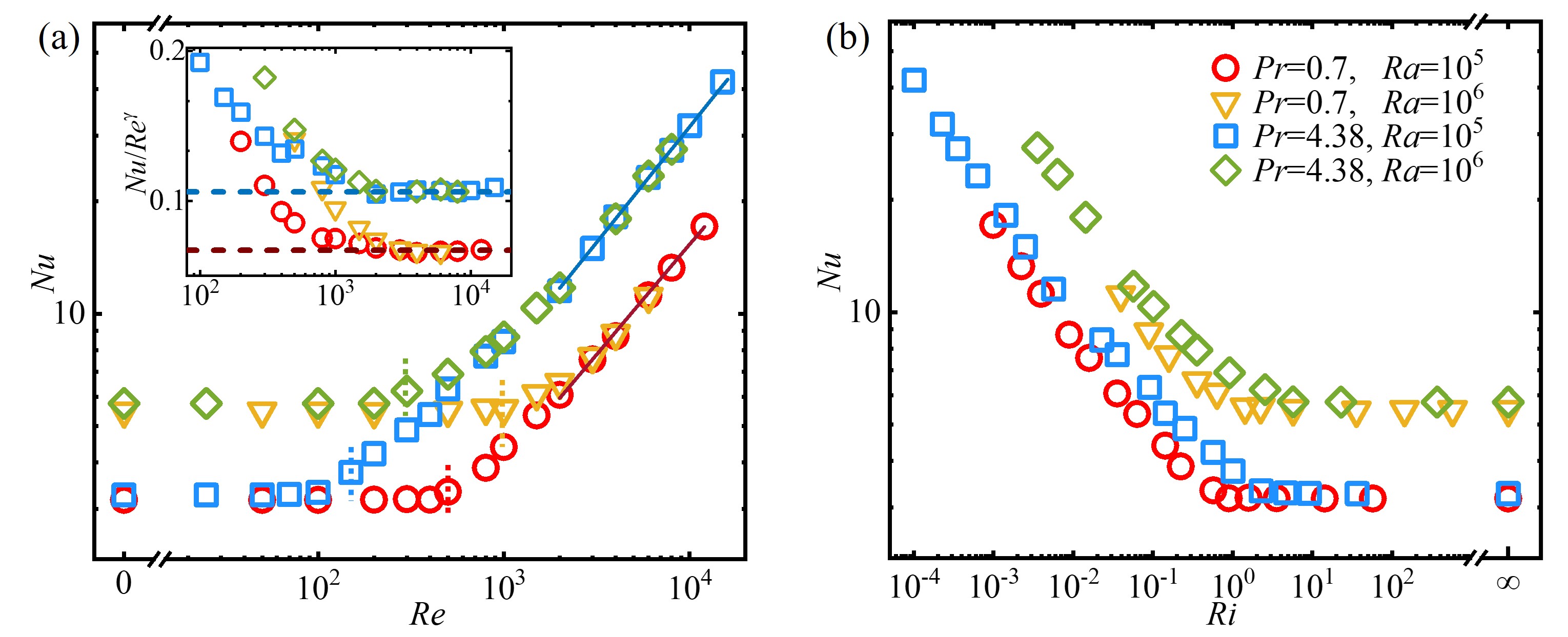
We first examine the global transport of heat. Data of the Nusselt number $Nu$ are shown as a function of $Re$ in Fig. 1(a) for $Ra=(10^{5}$ , $10^{6})$ and $Pr=(0.7$ , $4.38)$ . Without or with weak rotations ( $0\leq Re\leq 100$ ), the flow and heat transfer are dominated by vertical convection [45], and $Nu$ is nearly independent of $Re$ . We see that in this buoyancy-dominant flow regime $Nu$ is larger for a greater $Ra$ for a given $Re$ , but nearly independent of $Pr$ . With increasing $Re$ , $Nu$ starts to grow when $Re$ exceeds a critical value $Re_{1}^{*}$ given in Table 1. Interestingly, $Nu$ for each $Pr$ converges and becomes independent of $Ra$ , indicating the fading away of buoyancy-driven convection. Further increasing $Re$ , a second transition takes place at $Re^{*}_{2}$ , after which $Nu$ exhibits a power-law scaling $Nu\sim Re^{\gamma}$ with $\gamma=0.590\pm 0.025$ for $Pr=0.7$ and $\gamma=0.619\pm 0.015$ for $Pr=4.38$ (see the compensated plot in the inset of Fig. 1(a)). Both scalings for $Pr=0.7$ and $4.38$ suggest the existence of a new flow regime for heat transfer. All the transitional values $Re^{*}_{1}$ and $Re^{*}_{2}$ are listed in Table 1. We find that at lower $Pr$ or higher $Ra$ , the more vigorously convective flows postpone the transitions.

We see in Fig. 1(a) the intriguing trend that in a TC system the radial heat transport $Nu$ is insensitive to the variation of $Pr$ in a low- $Re$ flow regime ( $Re\textless Re_{1}^{*}$ ), but becomes strongly dependent on $Pr$ (independent of $Ra$ ) with sufficiently high $Re$ . In the intermediate regime of $Re$ , our data curves of $Nu(Re)$ show complicated $Ra$ - and $Pr$ -dependence. To better clarify the variations of the heat transport with changing control parameters, we show in Fig. 1(b) the Nusselt number as a function of Richardson number $Ri$ which measures the relative strength of buoyancy and rotation. In a high- $Ri$ regime where the buoyancy-driven convection is dominant (corresponding to the low- $Re$ regime shown in Fig. 1(a)), we see that $Nu$ remains a constant. The first transition for $Nu$ -enhancement takes place at $Ri_{1}^{*}$ that depends on both $Ra$ and $Pr$ . When $Ri\leq Ri^{*}_{1}(Ra,Pr)$ , the strong rotations start to affect the flows and $Nu$ increases monotonically as $Ri$ decreases. In comparison with the complicated $Ra$ - and $Pr$ -dependence shown in Fig. 1(a), a clear trend is displayed: the curves of $Nu(Ri)$ collapse approximately for the same $Ra$ with various $Pr$ , but become well distinguishable when different $Ra$ is used. For a given $Ri$ , $Nu$ increases with increasing $Ra$ .

III.1.2 Angular momentum transport

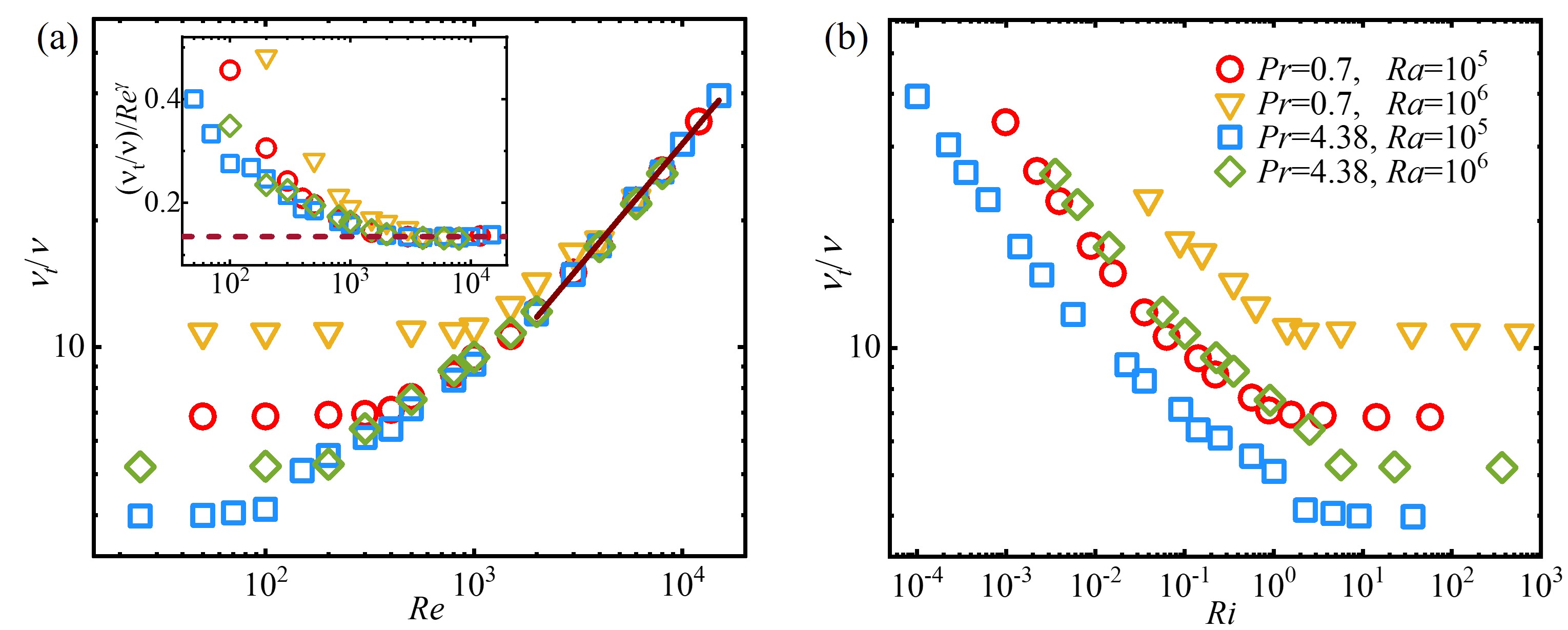
Figure 2(a) presents the dimensionless effective viscosity $\nu_{t}/\nu$ as functions of $Re$ for various $Pr$ and $Ra$ , which reveals the global angular momentum transport. In a low- $Re$ regime where vigorous convection governs the flows, $\nu_{t}/\nu$ is independent of $Re$ , but increases with a larger $Ra$ or with a smaller $Pr$ . Analogous to the heat transport data, we see that $\nu_{t}/\nu$ starts to increase when $Re$ exceeds the transitional value $Re_{1}^{*}(Ra,Pr)$ obtained in Fig. 1(a). For various $Ra$ and $Pr$ , data of $\nu_{t}/\nu(Re)$ converge to the same curve for $Re\textgreater Re_{1}^{*}$ , and follow a unifying power-law scaling $\nu_{t}/\nu\sim Re^{0.588\pm 0.038}$ after the second transition for $Re\textgreater Re^{*}_{2}$ (see the compensated plot in inset). In Fig. 2(b) where the data are plotted as a function of $Ri$ , we see that with decreasing $Ri$ , $\nu_{t}/\nu$ starts to increase at $Ri^{*}_{1}$ . Unlike the converging of $Nu(Ri)$ for a given $Ra$ and with varying $Pr$ as shown in Fig. 1(b), curves of $\nu_{t}/\nu(Ri)$ are found to be dependent on both $Ra$ and $Pr$ .

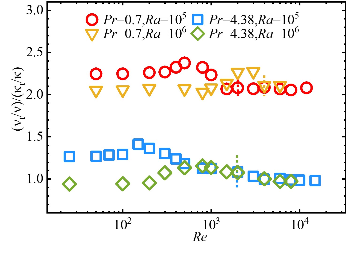
Further analyses are performed regarding the similar properties of heat and momentum transport for high Reynolds number. In Fig. 3, we show the ratio of the dimensionless effective viscosity $\nu_{t}/\nu$ to the diffusivity $\kappa_{t}/\kappa$ as a function of $Re$ . The dimensionless effective diffusivity is defined as ${\kappa_{t}}/{\kappa}=aNu$ , where $a=2d^{2}/(ln(r_{2}/r_{1})(r_{2}^{2}-r_{1}^{2}))$ is the geometry factor (Appendix B). It is found that, the ratio remains approximately a constant close to unity irrespective of $Ra$ for $Pr=4.38$ when $Re\textgreater Re_{2}^{*}$ . The ratio appears larger for a lower $Pr$ .

For each set of $Ra$ and $Pr$ , we have seen from above that the Reynolds-number dependences of heat and angular momentum transport exhibit a similar trend, and the transitions of different transport regimes take place at same critical values of $Re_{1}^{*}$ and $Re_{2}^{*}$ . These results suggest that, there is a unified mechanism that governs the processes of both heat and angular momentum transport in the present system. In the following, we will gain some insights into the transport properties by analysing the flow morphology and structures in different flow regimes.

III.2 Flow morphology

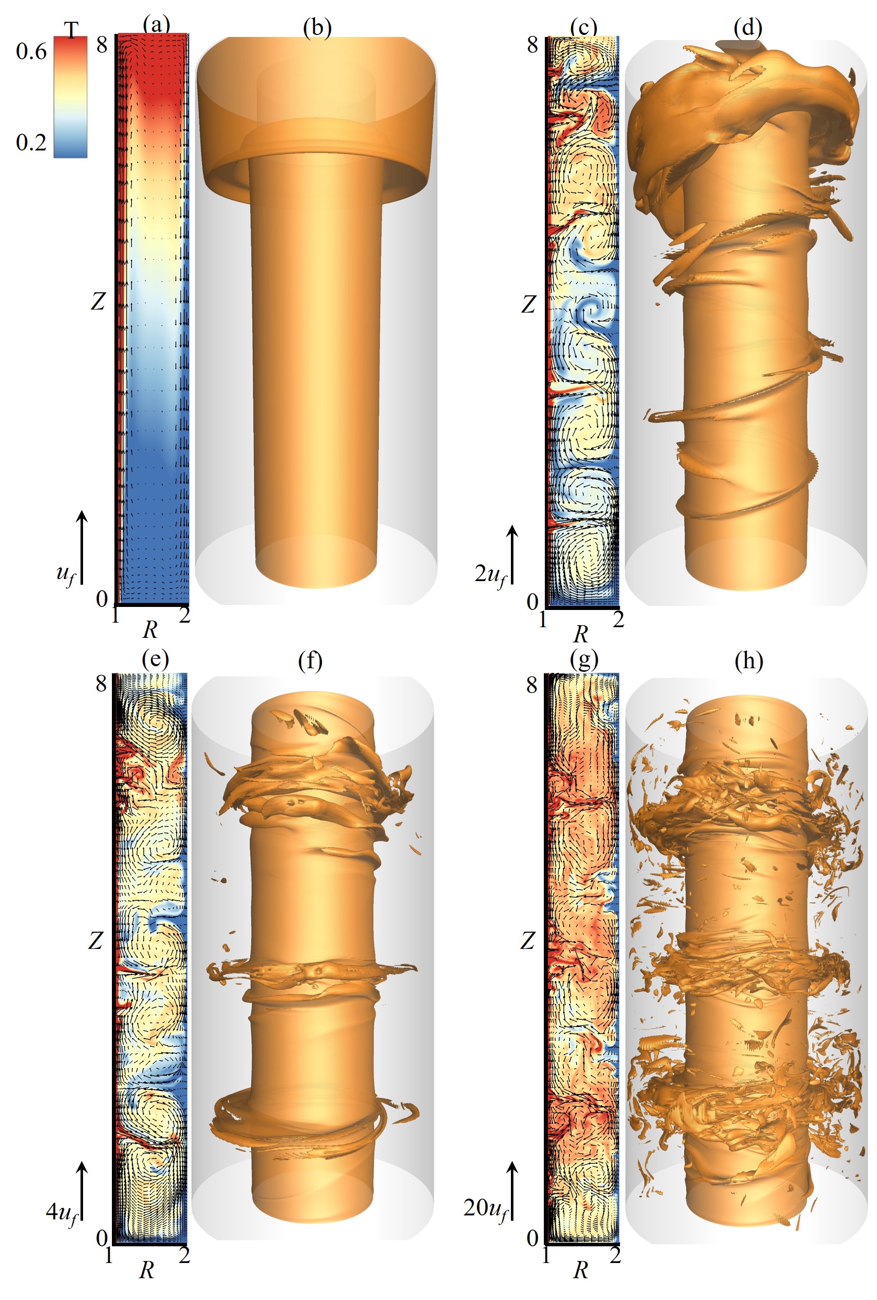
To illustrate the evolution of flow structures, we show two- and three-dimensional temperature fields in Fig. 4. Without rotations ( $Re=0$ as seen in Figs. 4(a) and (b)), the convective structure is axisymmetric, with a large-scale meridional circulation carrying ascending hot flows along the inner cylinder and descending cold flows along the outer cylinder. These are the typical temperature distributions in vertical convection [45, 46, 47]. For $Re\textless Re_{1}^{*}$ , since the rotation is too weak to affect the circulation, we thus see that the $Nu$ and $\nu_{t}/\nu$ remain at their non-rotating values shown in Figs. 1 and 2. When the rotation effect becomes comparable to the buoyancy for $Re\geq Re^{*}_{1}$ , the flow undergoes the first transition from the meridional circulation to spiral vortices (see Figs. 4(c) and (d)), which starts to enhance the radial transport of heat and angular momentum. In this rotation-affected regime, we find that both the flow morphology and the transport properties are dependent on both $Ra$ and $Pr$ . With further increase in $Re$ , rotation gradually dominates buoyancy, and the spiral vortices are replaced by the toroidal TVs (see Figs. 4(e) and (f)). In this TC-dominated regime $Nu(Re)$ and $\nu_{t}/\nu(Re)$ collapse respectively onto one curve that is independent of $Ra$ (Figs. 1(a) and 2(a)). The spiral vortices exist in an intermediate $Ri$ -regime $0.089\leq Ri\leq 2.54$ depending on $Ra$ and $Pr$ . In a similar system [48], the onset of spiral flow is reported in the range of $0.12\textless Ri\textless 0.47$ , showing a reasonable consistency with the present results. We note that the convection states of co-rotating and counter-rotating vortices reported in Ref. [28] are not observed in the present study, presumably due to the different geometry of fluid domain used in the present study.

Table 1: A summary of the transitional values

Re_{1}^{*}

(

Ri_{1}^{*}

) and

Re_{2}^{*}

(

Ri_{2}^{*}

	$Re_{1}^{}$ ( $Ri_{1}^{}$ )	$Re_{2}^{}$ ( $Ri_{2}^{}$ )
$Ra=10^{5},Pr=0.7$	500(0.57)	2000(0.036)
$Ra=10^{5},Pr=4.38$	150(1.01)	2000(0.006)
$Ra=10^{6},Pr=0.7$	1000(1.43)	4000(0.089)
$Ra=10^{6},Pr=4.38$	300(2.54)	2000(0.057)

We see that with sufficiently large Reynolds number $Re\geq Re_{2}^{*}$ , the flow undergoes the second transition to the turbulent TV flow (Figs. 4(g) and (h)), which is in good accord with previous studies in adiabatic TC systems [37] and in TC systems with a vertical temperature gradient applied [33]. In this flow regime, the turbulent transport of heat and momentum follows a unifying power-law scaling as shown in Figs. 1(a) and 2(a). In contrast to the flow fields with a lower $Re$ $(Re\textless Re_{2}^{*})$ , we can see that the temperature field with $Re\geq Re_{2}^{*}$ consists of rich small-scale structures, with hot fluids pumped more efficiently into the bulk flow from the inner cylinder, resulting in a higher transport efficiency. Note that for $Ra=10^{6}$ and $Pr=0.7$ the vigorous buoyancy-driven turbulence largely postpones the second transition $Re^{*}_{2}$ . We thus find that the spiral vortices can persist for $Re\textgreater 2000$ , and then turn into the turbulent TVs directly when $Re\textgreater 4000$ .

III.3 Mutual coherent structures for heat and angular momentum transport

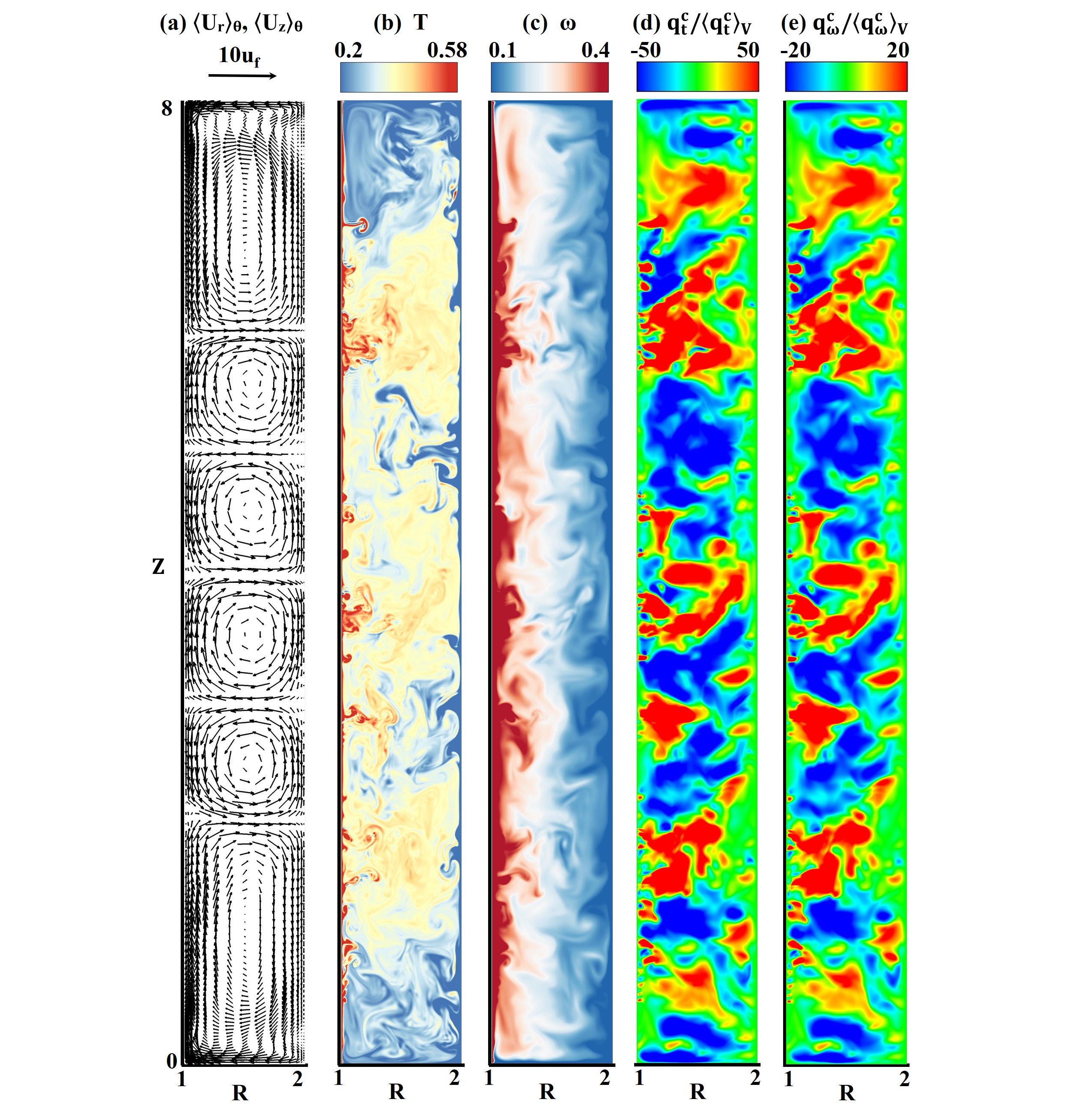
In this section, we demonstrate that mutual coherent structures in forms of turbulent TVs exist, through which both heat and angular momentum are transported efficiently in the high- $Re$ flow regime. To verify this viewpoint, we present in Fig. 5 the flow fields and the spatial distributions of heat and angular velocity fluxes, respectively. In Fig. 5(a), three pairs of TVs characterize the time-averaged velocity field. The instantaneous temperature field shown in Fig. 5(b), however, is dominated by turbulent fluctuations. TVs can be recognized roughly as the hot (cold) plumes which are emanating from the inner (outer) cylinder towards the bulk flow. In the instantaneous fields of $\omega$ (Fig. 5(c)), we observe large-scale coherent structures, while TVs are hard to be identified. In Figs. 5(d) and (e) we further show the spatial distributions of convective flux densities of heat ( $q^{c}_{t}/\left\langle q^{c}_{t}\right\rangle_{V}$ ) and angular velocity ( $q^{c}_{\omega}/\left\langle q^{c}_{\omega}\right\rangle_{V}$ ), normalized by their averaged values (see definitions of flux densities in Appendix B). We can see that both the instantaneous flux densities exhibit a similar spatial distribution. Therefore, we conjecture that the turbulent heat and angular momentum transport are archived through mutual coherent structures in the high- $Re$ regime.

To gain more insight into the mutual coherent structures for heat and angular momentum transport, we present data analysis of the spatial distribution of the local flux densities. We denote each spatial position of the fluid domain studied as $P(r,\theta,z)$ . Following the strategy used in Refs. [49, 50], we identify the pronounced structures of efficient turbulent transport, determining the spatial regions where the flux densities ( $q^{c}_{t}$ , $q^{c}_{\omega}$ ) are greater than their averaged values ( $\left\langle q^{c}_{t}\right\rangle_{V}$ , $\left\langle q^{c}_{\omega}\right\rangle_{V}$ ). Thus, for heat transport we define $(i)$ hot plumes $P_{t,hot}(r,\theta,z)$ where $q^{c}_{t}(r,\theta,z)\geq C\cdot\left\langle q^{c}_{t}\right\rangle_{V}$ and $(ii)$ cold plumes $P_{t,cold}(r,\theta,z)$ where $q^{c}_{t}(r,\theta,z)\leq-C\cdot\left\langle q^{c}_{t}\right\rangle_{V}$ . Similarly, for angular velocity transport, we define $(iii)$ “hot” (positive) plumes $P_{{\omega},hot}(r,\theta,z)$ where $q^{c}_{\omega}(r,\theta,z)\geq C\cdot\left\langle q^{c}_{\omega}\right\rangle_{V}$ and $(iv)$ “cold” (negative) plumes $P_{{\omega},cold}(r,\theta,z)$ where $q^{c}_{\omega}(r,\theta,z)\leq-C\cdot\left\langle q^{c}_{\omega}\right\rangle_{V}$ . The first subscript ( $t$ , $\omega$ ) denotes heat and angular velocity, and the second subscript ( $hot$ , $cold$ ) denotes the hot and cold plumes respectively. The factor $C$ is an empirical parameter chosen to be in the range of $1\leq C\leq 40$ in this study. The mutual coherent structures are then defined as the overlapping volume of $P_{{t}}(r,\theta,z)$ and $P_{{\omega}}(r,\theta,z)$ as follows, $(v)$ the mutual hot plumes $P_{t,\omega,hot}(r,\theta,z)$ where $q^{c}_{t}(r,\theta,z)\geq C\cdot\left\langle q^{c}_{t}\right\rangle_{V}$ and $q^{c}_{\omega}(r,\theta,z)\geq C\cdot\left\langle q^{c}_{\omega}\right\rangle_{V}$ , and $(vi)$ the mutual cold plumes $P_{t,\omega,cold}(r,\theta,z)$ where $q^{c}_{t}(r,\theta,z)\leq-C\cdot\left\langle q^{c}_{t}\right\rangle_{V}$ and $q^{c}_{\omega}(r,\theta,z)\leq-C\cdot\left\langle q^{c}_{\omega}\right\rangle_{V}$ . Through time- and volume-averaging, we obtain the mean volumes of the hot plumes

\displaystyle V_{t,hot}=(V_{0}\tau_{0})^{-1}\int_{V,\tau}P_{t,hot}dVd\tau,\quad V_{\omega,hot}=(V_{0}\tau_{0})^{-1}\int_{V,\tau}P_{\omega,hot}dVd\tau,

(3)

the cold plumes

\displaystyle V_{t,cold}=(V_{0}\tau_{0})^{-1}\int_{V,\tau}P_{t,cold}dVd\tau,\quad V_{\omega,cold}=(V_{0}\tau_{0})^{-1}\int_{V,\tau}P_{\omega,cold}dVd\tau,

(4)

and the mutual plumes

\displaystyle V_{t,\omega,hot}=(V_{0}\tau_{0})^{-1}\int_{V,\tau}P_{t,\omega,hot}dVd\tau,\quad V_{t,\omega,cold}=(V_{0}\tau_{0})^{-1}\int_{V,\tau}P_{t,\omega,cold}dVd\tau,

(5)

where $V_{0}=\int_{V}PdV$ and $\tau_{0}$ denote the whole volume and time period.

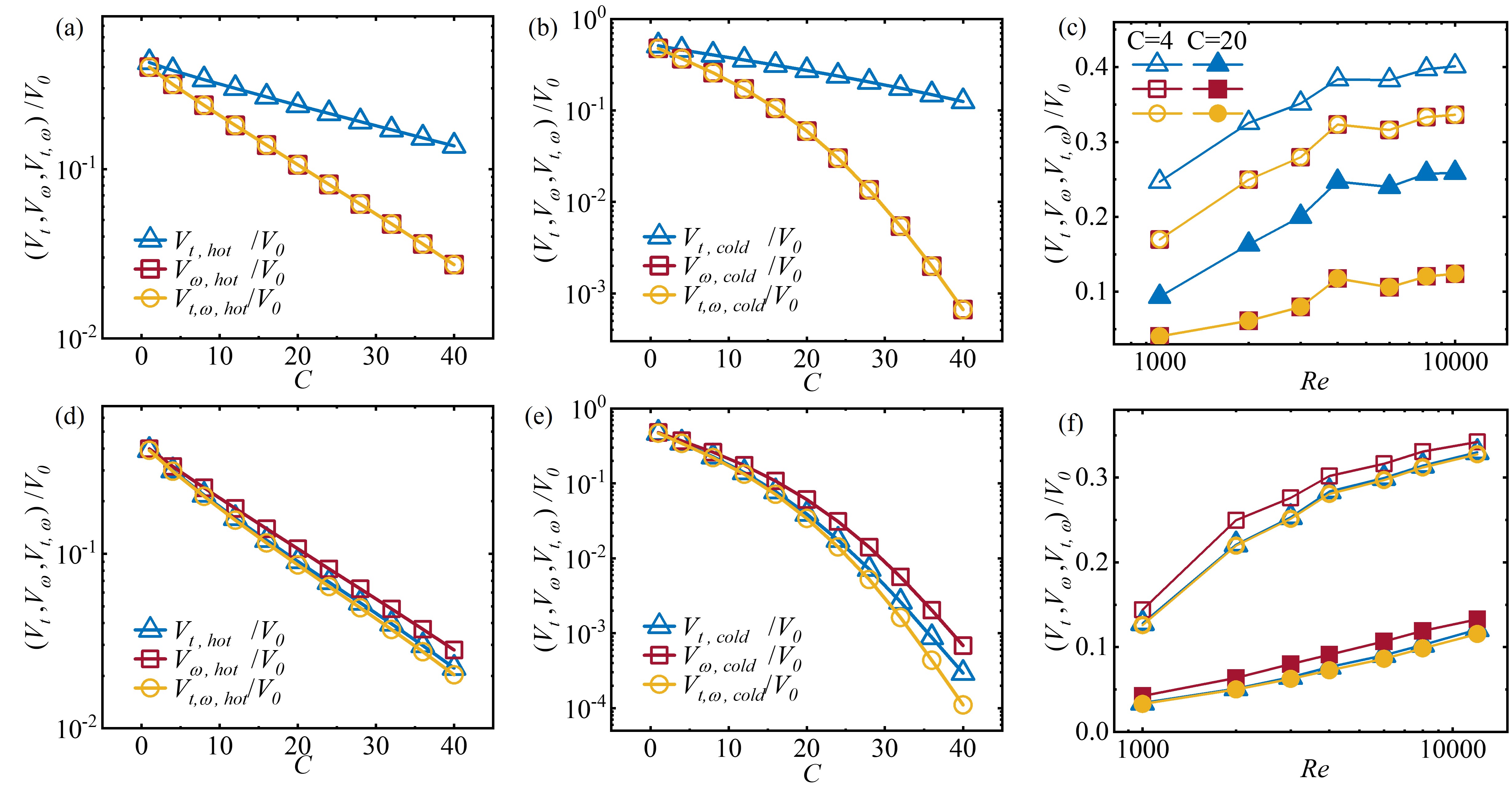
The volume ratios $V_{t}/V_{0}$ , $V_{\omega}/V_{0}$ and $V_{t,\omega}/V_{0}$ for $Pr=4.38$ are plotted as functions of $C$ in Figs. 6(a) and (b). As shown in Fig. 6(a), these ratios for hot plumes are about 0.42 for $C=1$ , and decrease as $C$ increases. Interestingly, data of the ratios $V_{\omega,hot}/V_{0}$ and $V_{t,\omega,hot}/V_{0}$ collapse, both decreasing more rapidly than $V_{t,hot}/V_{0}$ . A similar trend is shown in Fig. 6(b) for the volume ratios of cold plumes. We see that the ratios of thermal plumes $V_{t,hot}/V_{0}$ and $V_{t,cold}/V_{0}$ are always greater than the angular-velocity and the mutual ones, indicating a broader distribution of thermal structures. In Fig. 6(c), the volume ratios of hot (positive) plumes are plotted as functions of $Re$ for two values of $C$ . We see that with increasing $Re$ the ratios $V_{t,hot}/V_{0}$ , $V_{\omega,hot}/V_{0}$ and $V_{t,\omega,hot}/V_{0}$ first increase and then become independent of $Re$ when $Re\geq 4000$ .

For the flows with low $Pr=0.7$ (Figs. 6(d), (e) and (f)), the data show almost similar trends when the parameters $C$ and $Re$ change. We see that the volume ratios become greater when $Re$ increases, or when $C$ decreases. However, here we find that $V_{\omega}/V_{0}$ becomes slightly greater than $V_{t}/V_{0}$ and $V_{t,\omega}/V_{0}$ for low $Pr$ . We attribute these to the $Pr$ -dependence of the flow properties, since heat is more likely to accumulate within the turbulent coherent structures for high $Pr=4.38$ , but becomes easier to diffuse for low $Pr=0.7$ . Results in Fig. 6 imply that in the high- $Re$ regime heat and angular momentum are transferred mainly through highly similar coherent structures. The flow regions of large angular momentum fluxes are nested within the regions of large heat fluxes for high $Pr=4.38$ , and vice versa for low $Pr=0.7$ . We suggest that it is the similarities of the turbulent structures, which deliver efficiently both the heat and angular momentum transport, give rise to the same scaling properties of $Nu$ and $\nu_{t}/\nu$ observed in Figs. 1, 2 and 3.

IV Concluding remarks

We investigate numerically the heat and angular momentum transport processes in the turbulent Taylor-Couette flows which are subjected to a radial temperature gradient. A large range of Reynolds number is considered, extending the present study of the heat transport to the unexplored regime of turbulent TVs.

We find that the flows undergo a first transition at $Re^{*}_{1}$ from the convection-dominated state in the form of a large-scale meridional circulation to the transitional regime typified by spiral vortices. After this transition we observe enhanced transport of heat and angular momentum, since rotations start to influence the flow structures. With increasing $Re$ , the flow turns into the TC-dominated regime where the heat and angular momentum transport become independent of $Ra$ . Eventually, the turbulent TVs start to dominate the turbulent transport processes at the second transition $Re^{*}_{2}$ , after which the heat and angular momentum transport are dictated by power-law scalings, i.e., $Nu\sim Re^{0.619\pm 0.015}$ for $Pr=4.38$ , $Nu\sim Re^{0.590\pm 0.025}$ for $Pr=0.7$ and $\nu_{t}/\nu\sim Re^{0.588\pm 0.036}$ for both $Pr$ . Our results also show that the transitional values $Re^{*}_{1}$ and $Re^{*}_{2}$ depend on both $Ra$ and $Pr$ .

A striking finding is the analogy between the radial transport of heat and angular momentum. Besides their similar scaling exponents, our data show that the effective viscosity ( $\nu_{t}/\nu$ ) and diffusivity ( $\kappa_{t}/\kappa$ ) have almost the same efficiency for $Re\textgreater 2000$ . The similar properties of both types of transport are found to persist in the turbulent TV regime, which was attributed to the mutual structures through which heat and momentum are efficiently transported. Further analysis shows that the structures for high-efficiency angular momentum transport are nested inside the thermal ones for high $Pr=4.38$ , or vice versa for low $Pr=0.7$ . We note that the analogy between heat and momentum transport in rotating flow has been interpreted through the one-dimensional simplified model by Bradshaw [51]. To further connect the present results with Bradshaw’s analogy is an intriguing subject for future studies. In a TC system where an axial destabilized temperature gradient is applied, it has been reported that, the axial heat transport has the same scaling as the radial angular momentum transport in the turbulent TV regime [33]. Hence, we suggest that it is the structures in forms of turbulent TVs that provide the TC systems with the equal transport efficiencies in both the radial and axial directions.

The ultimate regime of TC flows [52, 53] sets in at a much larger Reynolds number ( $Re\textgreater 6\times 10^{4}$ for $\eta=0.5$ [38, 34, 35]) than the parameters considered in the present study. Whether a similar scaling of heat and angular momentum transport exists at higher $Re$ and even in the ultimate regime, remains a challenging problem for future studies.

Acknowledgements.

This work was supported by the Natural Science Foundation of China under grant nos. 11902224, 11772235 and the China Postdoctoral Science Foundation (No.2019M651572).

Appendix A Numerical details

A.1 Grid sensitivity studies and main results

The results of the grid sensitivity studies are listed in Table 2. It is shown that, results of $Nu$ and $Re_{\tau}$ show a good convergence as resolutions increase. The main results are listed in Tables 3 and 4. For all our runs, the smallest mean scales are respectively determined by the mean Kolmogrov scale $\left\langle\lambda_{k}\right\rangle_{V}=(\nu^{3}/\left\langle{\epsilon_{\nu}}\right\rangle_{V})^{1/4}$ for $Pr=0.7$ , and the mean Batchelor scale $\left\langle\lambda_{b}\right\rangle_{V}=(\kappa^{2}\nu/\left\langle{\epsilon_{\nu}}\right\rangle_{V})^{1/4}$ for $Pr=4.38$ , where $\left\langle{\epsilon_{\nu}}\right\rangle_{V}$ is the volume- and time-averaged turbulent kinetic energy dissipation rate [54, 55, 56, 57]. At high Reynolds number, the flow enters into the shear-dominated regime, that $\left\langle\lambda_{b}\right\rangle_{V}$ decreases rapidly with the increasing kinetic energy dissipation. Thus, the ratios of the greatest grid spacing $L_{max}$ [58] to $\left\langle\lambda_{k}\right\rangle_{V}$ and $\left\langle\lambda_{b}\right\rangle_{V}$ [59] do not exceed 2.7 and 4.5 respectively in this study. Meanwhile, the minimal radial grid spacing in wall units is always less than unit. Besides this, the relative error measurement $\sigma_{\epsilon_{T}}$ is employed to check the deviation of the exact balance between the thermal dissipation and the global heat transfer [60, 56, 57]. To reduce the computational requirements for high- $Re$ flows, the azimuthal computational extents $L_{\theta}$ are reduced to a quarter of the cylinder ( $0.5\pi$ ) for $Re\geq 4000$ . This strategy has been proven to be effective [61, 62]. And as shown in Tables 3 and 4, the simulations for $L_{\theta}=2\pi$ and $0.5\pi$ are both performed in the range of $1000\leq Re\leq 4000$ , and the results suggest that the shortened extents do not change the main results.

In Tables 2, 3 and 4, $N_{\theta}{\times}{N_{z}}{\times}N_{r}$ denote the resolutions in three directions, and $L_{\theta}$ is the azimuthal computational extent; $\sigma_{\epsilon_{T}}$ is the relative error measured by $Nu$ and the thermal dissipation rate; $\frac{L_{max}}{\left\langle\lambda_{k}\right\rangle_{V},\left\langle\lambda_{b}\right\rangle_{V}}$ are the maximal grid spacings compared with the Kolmogrov and Batchelor scales; $r^{+}_{min},r^{+}_{max}$ are the minimal and maximal grid sizes in wall units.

A.2 Discussions of the centrifugal buoyancy effects

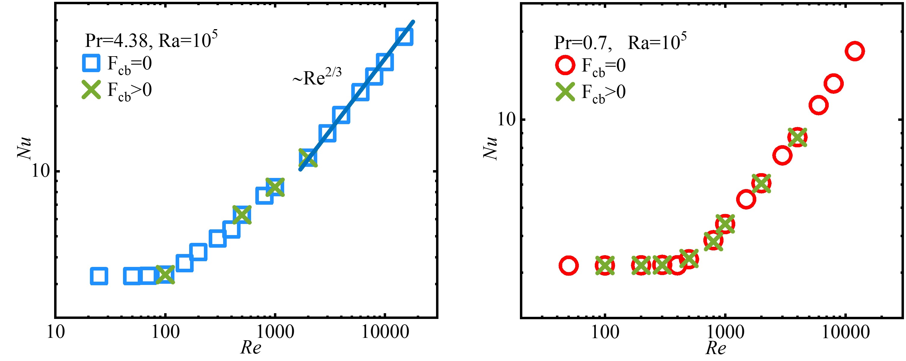
In our system, the centrifugal buoyancy $F_{cb}=-(\beta\Delta)({U_{\theta}^{2}}/{R})T{\mathit{e_{r}}}$ [26, 28] is present because of the azimuthal motion of the fluid. Here we perform the additional simulations for the experimental conditions with $\beta\approx 0.004K^{-1}$ and $\Delta=10K$ for air and with $\beta\approx 0.00038K^{-1}$ and $\Delta=10K$ for water. The results shown in Fig. 7 indicate that, including the centrifugal buoyancy does not change the results of heat transport. Therefore, in this paper, the effect of centrifugal force is neglected.

A.3 Comparison with experimental results

To validate our results for high- $Re$ regime, we compare the heat-transport data with the previous experimental results in Fig. 6(a). Our results are consistent with the power-law scaling obtained in Ref. [63] for $2000\leq Re\textless 10000$ . But for high $Re\textgreater 10000$ , it is found that $Nu$ tends to deviate from the scaling law. We argue that the difference results from their fitting errors, since this scaling exponent is already same to the well-accept value ( $\textgreater 2/3$ ) for ultimate turbulent regime [4].

Table 2: A summary of the grid sensitivities study for

Ra=10^{5}

Re=8000

and

Pr=0.7

$N_{\theta}(L_{\theta}){\times}N_{z}{\times}N_{r}$	$Nu$	$Re_{\tau}$	$\sigma_{\epsilon_{T}}$	$L_{max}/(\left\langle\lambda_{k}\right\rangle_{V},\left\langle\lambda_{b}\right\rangle_{V})$
$128(0.5\pi)\times 1025\times 225$	13.54	232.95	0.02	2.45, 2.05
$192(0.5\pi)\times 1537\times 225$	13.29	229.24	0.01	1.86, 1.56
$256(0.5\pi)\times 2049\times 225$	13.20	229.53	0.01	1.51, 1.26

Table 3: A summary of the main results for

Pr=4.38

$Re$	$Pr$	$Ra$	$N_{\theta}(L_{\theta}){\times}N_{z}{\times}N_{r}$	$Nu$	$Re_{\tau}$	$\sigma_{\epsilon_{T}}$	$L_{max}/(\left\langle\lambda_{k}\right\rangle_{V},\left\langle\lambda_{b}\right\rangle_{V})$	$r^{+}_{min},r^{+}_{max}$
0	4.38	$10^{5}$	$128(2\pi)\times 257\times 33$	3.27	$-$	0.00	0.90, 1.89	$-$ , $-$
25	4.38	$10^{5}$	$128(2\pi)\times 257\times 33$	3.27	4.99	0.00	0.91, 1.91	0.07, 0.59
50	4.38	$10^{5}$	$128(2\pi)\times 257\times 33$	3.27	7.06	0.00	0.94, 1.96	0.10, 0.84
70	4.38	$10^{5}$	$128(2\pi)\times 257\times 33$	3.28	8.42	0.00	0.97, 2.02	0.12, 1.00
100	4.38	$10^{5}$	$128(2\pi)\times 257\times 33$	3.32	10.16	0.00	1.02, 2.13	0.14, 1.20
150	4.38	$10^{5}$	$128(2\pi)\times 257\times 33$	3.75	13.83	0.01	1.14, 2.39	0.19, 1.64
200	4.38	$10^{5}$	$128(2\pi)\times 321\times 41$	4.22	16.64	0.01	1.27, 2.66	0.23, 1.72
300	4.38	$10^{5}$	$128(2\pi)\times 321\times 41$	4.88	21.41	0.01	1.33, 2.79	0.23, 1.77
400	4.38	$10^{5}$	$128(2\pi)\times 321\times 41$	5.37	25.29	0.02	1.54, 3.22	0.27, 2.40
500	4.38	$10^{5}$	$128(2\pi)\times 321\times 41$	6.28	29.89	0.02	1.77, 3.69	0.32, 2.83
800	4.38	$10^{5}$	$128(2\pi)\times 385\times 49$	7.70	40.88	0.02	2.05, 4.29	0.36, 3.23
1000	4.38	$10^{5}$	$192(2\pi)\times 513\times 65$	8.43	47.74	0.02	1.76, 3.69	0.23, 3.09
1000	4.38	$10^{5}$	$64(0.5\pi)\times 513\times 65$	8.47	47.89	0.02	1.60, 3.36	0.23, 3.10
2000	4.38	$10^{5}$	$256(2\pi)\times 721\times 91$	11.63	77.46	0.03	1.93, 4.04	0.26, 3.57
2000	4.38	$10^{5}$	$96(0.5\pi)\times 721\times 91$	11.74	77.65	0.03	1.69, 3.54	0.26, 3.58
3000	4.38	$10^{5}$	$128(0.5\pi)\times 897\times 129$	14.98	105.63	0.04	1.64, 3.42	0.25, 3.42
4000	4.38	$10^{5}$	$128(0.5\pi)\times 1025\times 161$	18.16	131.90	0.04	1.74, 3.65	0.25, 3.42
6000	4.38	$10^{5}$	$192(0.5\pi)\times 1281\times 193$	23.19	183.50	0.04	1.73, 3.62	0.29, 3.96
8000	4.38	$10^{5}$	$256(0.5\pi)\times 1537\times 225$	27.40	228.16	0.03	1.69, 3.53	0.30, 4.20
10000	4.38	$10^{5}$	$256(0.5\pi)\times 1793\times 257$	31.90	275.04	0.04	1.77, 3.71	0.32, 4.46
15000	4.38	$10^{5}$	$256(0.5\pi)\times 2001\times 301$	41.79	384.76	0.04	2.11, 4.43	0.38, 5.32
0	4.38	$10^{6}$	$256(2\pi)\times 513\times 65$	5.75	$-$	0.00	0.93, 1.95	$-$ , $-$
25	4.38	$10^{6}$	$256(2\pi)\times 513\times 65$	5.75	5.70	0.00	0.93, 1.95	0.04, 0.34
100	4.38	$10^{6}$	$256(2\pi)\times 513\times 65$	5.75	11.42	0.00	0.94, 1.97	0.07, 0.68
200	4.38	$10^{6}$	$256(2\pi)\times 513\times 65$	5.76	16.25	0.00	0.97, 2.03	0.11, 0.96
300	4.38	$10^{6}$	$256(2\pi)\times 513\times 65$	6.21	21.93	0.00	1.01, 2.11	0.14, 1.30
500	4.38	$10^{6}$	$256(2\pi)\times 513\times 65$	6.89	30.66	0.01	1.15, 2.42	0.20, 1.82
800	4.38	$10^{6}$	$256(2\pi)\times 513\times 65$	7.92	41.98	0.02	1.46, 3.06	0.20, 2.72
1000	4.38	$10^{6}$	$256(2\pi)\times 513\times 65$	8.67	48.69	0.03	1.64, 3.43	0.24, 3.15
1500	4.38	$10^{6}$	$256(2\pi)\times 641\times 81$	10.37	63.72	0.03	1.77, 3.69	0.24, 3.25
2000	4.38	$10^{6}$	$384(2\pi)\times 721\times 91$	11.75	77.97	0.02	1.69, 3.55	0.27, 3.59
4000	4.38	$10^{6}$	$128(0.5\pi)\times 1025\times 161$	17.97	131.67	0.04	1.74, 3.65	0.25, 3.42
6000	4.38	$10^{6}$	$192(0.5\pi)\times 1281\times 193$	23.38	181.11	0.04	1.72, 3.60	0.28, 3.90
8000	4.38	$10^{6}$	$256(0.5\pi)\times 1537\times 225$	27.40	228.16	0.03	1.69, 3.53	0.30, 4.20

Table 4: A summary of the main results for

Pr=0.7

$Re$	$Pr$	$Ra$	$N_{\theta}(L_{\theta}){\times}N_{z}{\times}N_{r}$	$Nu$	$Re_{\tau}$	$\sigma_{\epsilon_{T}}$	$L_{max}/(\left\langle\lambda_{k}\right\rangle_{V},\left\langle\lambda_{b}\right\rangle_{V})$	$r^{+}_{min},r^{+}_{max}$
0	0.7	$10^{5}$	$128(2\pi)\times 257\times 33$	3.17	$-$	0.00	2.36, 1.98	$-$ , $-$
50	0.7	$10^{5}$	$128(2\pi)\times 257\times 33$	3.17	9.26	0.00	2.37, 1.99	0.10, 1.19
100	0.7	$10^{5}$	$128(2\pi)\times 257\times 33$	3.17	13.06	0.00	2.38, 1.99	0.14, 1.69
200	0.7	$10^{5}$	$128(2\pi)\times 321\times 41$	3.18	18.59	0.00	2.09, 1.75	0.15, 1.92
300	0.7	$10^{5}$	$128(2\pi)\times 321\times 41$	3.19	22.83	0.00	2.15, 1.80	0.18, 2.36
400	0.7	$10^{5}$	$128(2\pi)\times 321\times 41$	3.18	26.66	0.00	2.23, 1.86	0.22, 2.76
500	0.7	$10^{5}$	$128(2\pi)\times 321\times 41$	3.33	30.87	0.01	2.30, 1.92	0.25, 3.19
800	0.7	$10^{5}$	$128(2\pi)\times 385\times 49$	3.87	41.59	0.01	2.32, 1.94	0.28, 3.58
1000	0.7	$10^{5}$	$192(2\pi)\times 513\times 65$	4.40	48.59	0.01	2.10, 1.76	0.23, 3.12
1000	0.7	$10^{5}$	$64(0.5\pi)\times 513\times 65$	4.38	48.19	0.01	1.65, 1.38	0.23, 3.09
1500	0.7	$10^{5}$	$192(2\pi)\times 641\times 81$	5.34	63.12	0.01	1.95, 1.63	0.24, 3.27
2000	0.7	$10^{5}$	$256(2\pi)\times 721\times 91$	6.06	77.91	0.01	2.14, 1.79	0.27, 3.59
2000	0.7	$10^{5}$	$96(0.5\pi)\times 721\times 91$	6.10	78.25	0.00	1.94, 1.63	0.27, 3.60
3000	0.7	$10^{5}$	$96(0.5\pi)\times 897\times 113$	7.55	106.18	0.01	1.89, 1.58	0.29, 3.93
4000	0.7	$10^{5}$	$256(2\pi)\times 1025\times 161$	8.70	132.14	0.01	2.20, 1.84	0.25, 3.43
4000	0.7	$10^{5}$	$128(0.5\pi)\times 1025\times 161$	8.88	133.44	0.01	1.75, 1.47	0.25, 3.46
6000	0.7	$10^{5}$	$128(0.5\pi)\times 1281\times 193$	11.20	182.83	0.01	1.98, 1.66	0.28, 3.95
8000	0.7	$10^{5}$	$192(0.5\pi)\times 1537\times 225$	13.29	229.24	0.01	1.86, 1.56	0.31, 4.25
12000	0.7	$10^{5}$	$192(0.5\pi)\times 1793\times 257$	17.13	320.74	0.02	2.20, 1.84	0.37, 5.20
0	0.7	$10^{6}$	$256(2\pi)\times 513\times 65$	5.49	$-$	0.00	2.41, 2.01	$-$ , $-$
50	0.7	$10^{6}$	$256(2\pi)\times 513\times 65$	5.49	11.64	0.00	2.41, 2.00	0.06, 0.75
100	0.7	$10^{6}$	$256(2\pi)\times 513\times 65$	5.48	16.47	0.00	2.41, 2.00	0.08, 0.89
200	0.7	$10^{6}$	$256(2\pi)\times 513\times 65$	5.48	23.34	0.00	2.42, 2.03	0.11, 1.5
500	0.7	$10^{6}$	$256(2\pi)\times 513\times 65$	5.48	37.44	0.00	2.45, 2.05	0.18, 2.40
800	0.7	$10^{6}$	$256(2\pi)\times 513\times 65$	5.52	46.68	0.00	2.48, 2.07	0.23, 3.02
1000	0.7	$10^{6}$	$256(2\pi)\times 513\times 65$	5.58	68.53	0.00	2.54, 2.13	0.26, 3.44
1500	0.7	$10^{6}$	$256(2\pi)\times 513\times 65$	6.11	68.60	0.01	2.66, 2.22	0.33, 4.44
2000	0.7	$10^{6}$	$256(2\pi)\times 721\times 91$	6.55	84.49	0.01	2.29, 1.92	0.29, 3.89
3000	0.7	$10^{6}$	$256(2\pi)\times 721\times 91$	7.67	112.20	0.01	2.68, 2.24	0.38, 5.17
4000	0.7	$10^{6}$	$256(2\pi)\times 1025\times 161$	8.84	133.96	0.02	1.89, 2.26	0.25, 3.47
6000	0.7	$10^{6}$	$128(0.5\pi)\times 1281\times 193$	11.12	184.46	0.02	1.73, 3.62	0.29, 3.96

Appendix B Derivations of flux densities, effective viscosity and diffusivity

In our annular system, the ring surface increases as $r$ increases, leading to a decreasing flux density along the radial direction. Hence, in this section the heat flux density $q_{t}$ and the angular velocity flux density $q_{\omega}$ are defined respectively, in addition to the common definitions of the heat and angular velocity currents.

B.1 Heat flux density $q_{t}$

Here, we consider the dimensional fields of velocity $\textbf{u}{(r,{\theta},z)}$ and temperature $t{(r,{\theta},z)}$ . For a pure thermal conductive state between the concentric cylinders, the one-dimensional radial temperature distribution is $t(r)=c_{1}lnr+c_{2}$ , with $c_{1}=-{\Delta}/{ln({r_{2}}/{r_{1}})}$ and $c_{2}=t_{2}-c_{1}ln(r_{2})$ . From Fourier’s law, the radial heat flux density (by thermal conduction) is $\mathit{q_{t}^{Lam}(r)}=-\kappa{\partial_{r}t}=-\kappa{c_{1}}/{r}$ , which decreases along the radial direction owing to the enlarging ring surface. For the turbulent flow, the three-dimensional distributions of the heat flux density is defined as,

\mathit{q_{t}{(r,{\theta},z)}}={u_{r}}{(r,{\theta},z)}(t{(r,{\theta},z)}-t_{2})-\kappa\partial_{r}{(t{(r,{\theta},z)}-t_{2})},

(6)

where the temperature of the cold wall $t_{2}$ is used as the reference temperature as done in Ref. [24]. The first term on the right-hand side corresponds to the convective contribution $q^{c}_{t}={u_{r}}{(r,{\theta},z)}(t{(r,{\theta},z)}-t_{2})$ . Thus the Nusselt number is defined as the ratio of the turbulent heat transport to the thermal conduction

Nu=\frac{\left\langle q_{t}\right\rangle_{V}}{\left\langle q_{t}^{Lam}\right\rangle_{V}}=a^{-1}({{\mathit{RePr}}\left\langle U_{r}T\right\rangle_{V}-\partial_{r}\left\langle{T}\right\rangle_{V}}),

(7)

where $a=2d^{2}/(ln(r_{2}/r_{1})(r_{2}^{2}-r_{1}^{2}))$ denotes the factor caused by the annular geometry.

B.2 Angular velocity flux density $q_{\omega}$

In circular Couette flow (CCF), the flow is laminar and has purely azimuthal velocity $u_{\theta}=Ar+{B}/{r}$ , with $A=({r_{2}u_{2}-r_{1}u_{1}})/({r_{2}^{2}-r_{1}^{2}})$ and $B=({r_{2}^{2}r_{1}u_{1}-r_{2}r_{1}^{2}u_{2}})/({r_{2}^{2}-r_{1}^{2}})$ . Thus, its angular velocity flux density could be written as $\mathit{q_{\omega}^{Lam}(r)}=2\nu{B}/{r}$ , which also decreases along the radial direction as same as $q_{t}^{Lam}$ . Taking into account the increasing area in the radial direction, after multiplication with $r$ , the conventional formula of the angular velocity current (for CCF) is $J_{\omega}^{Lam}=2\nu B$ [40]. In turbulent flows, according to the derivations from Ref. [40], the conventional angular velocity current is expressed as

\displaystyle\mathit{\left\langle J_{\omega}{(r,{\theta},z)}\right\rangle_{\theta z}}=r^{2}\left\langle{u_{r}}{(r,{\theta},z)}{u_{\theta}}{(r,{\theta},z)}\right\rangle_{\theta z}-\nu r^{3}\partial_{r}\left(\left\langle u_{\theta}{(r,{\theta},z)}\right\rangle_{\theta z}/{r}\right).

(8)

Here, without regard to the temporal and spatial averaging processes, the spatial distribution of $J_{\omega}$ is,

\displaystyle\mathit{J_{\omega}{(r,{\theta},z)}}=r^{2}{u_{r}}{(r,{\theta},z)}{u_{\theta}}{(r,{\theta},z)}-\nu r^{3}\partial_{r}\left(u_{\theta}{(r,{\theta},z)}/r\right).

(9)

When $J_{\omega}$ is divided by $r$ , one could obtain the definition of angular velocity flux density

\displaystyle\mathit{q_{\omega}{(r,{\theta},z)}}

\displaystyle=r{u_{r}}{(r,{\theta},z)}{u_{\theta}}{(r,{\theta},z)}-\nu r^{2}\partial_{r}\left(u_{\theta}{(r,{\theta},z)}/{r}\right).

(10)

The convective part is $q^{c}_{\omega}=r{u_{r}}{(r,{\theta},z)}{u_{\theta}}{(r,{\theta},z)}$ . It is worth noting that, $\left\langle J_{\omega}\right\rangle_{\theta z}$ is the commonly conserved transverse current, whereas the density $\left\langle q_{\omega}\right\rangle_{\theta z}$ decreases along the radial direction as same as the heat flux density.

B.3 Effective viscosity $\nu_{t}/\nu$ and diffusivity $\kappa_{t}/\kappa$

The global heat transfer could be defined as $Nu={Q_{t}}/{Q_{t}^{Lam}}$ , where $Q_{t}=\int_{V,\tau}q_{t}dVd\tau$ and $Q_{t}^{Lam}=\int_{V,\tau}q_{t}^{Lam}dVd\tau$ . To describe the contribution of turbulent transport to the global heat transfer, the effective thermal diffusivity $\kappa_{t}$ is defined as $Q_{t}=\int_{V,\tau}\kappa_{t}({\Delta}/{d})dVd\tau$ . Thus the dimensionless effective diffusivity is

\frac{\kappa_{t}}{\kappa}=aNu,

(11)

where $a=2d^{2}/(ln(r_{2}/r_{1})(r_{2}^{2}-r_{1}^{2}))$ .

In the axially periodical domain or very long cylinders, $\left\langle J_{\omega}\right\rangle_{\theta z}$ remains constant radially. However, owing to the braking effect of the fixed endwalls, $\left\langle J_{\omega}\right\rangle_{\theta z}$ decreases along the radial direction in our system. We consider the angular velocity flux at the inner cylinder the $\omega$ -Nusselt number for angular velocity transfer [33]

Nu_{\omega}=\frac{\left\langle J_{\omega}\right\rangle_{\theta z,r=r_{1}}}{J_{\omega}^{Lam}}=\frac{u_{1}d}{2B}\frac{(R_{1}^{2})(2Re_{\tau})^{2}}{Re},

(12)

where the friction Reynolds number $Re_{\tau}$ is defined as $Re_{\tau}=0.5u_{\tau}d/\nu$ with the friction velocity $u_{\tau}^{2}=-\nu r(\partial_{r}\left\langle u_{\theta}/r\right\rangle_{\theta z})$ at the inner wall. Following Lathrop’s estimation [31, 32], we define the effective viscosity (owing to the turbulent transport) $\nu_{t}=G_{r_{1}}/(2\pi\rho u_{1}r_{1}^{2}h{d^{-1}})$ , where the inner torque $G_{r_{1}}=2\pi r_{1}^{3}h\rho\nu{\partial_{r}}\left({\left\langle{u_{\theta}}/{r}\right\rangle_{\theta z}}\right)=2\pi r_{1}^{2}h{\rho\nu^{2}}{d^{-2}}(2Re_{\tau})^{2}$ . Thus, one could obtain the equation of the dimensionless effective viscosity [33]

\frac{\nu_{t}}{\nu}=\frac{(2Re_{\tau})^{2}}{Re}.

(13)

It is found that, the diffusivity $\kappa_{t}/\kappa$ and dimensionless effective viscosity $\nu_{t}/\nu$ have the same scaling with the global transport of heat ( $Nu$ ) and angular momentum ( $Nu_{\omega}$ ) respectively.

References

Hussain [1986] A. K. M. F. Hussain, Coherent structures and turbulence, J. Fluid Mech. 173, 303–356 (1986).
Bergman et al. [2011] T. Bergman, F. Incropera, D. DeWitt, and A. Lavine, Fundamentals of heat and mass transfer (John Wiley & Sons, 2011).
Holmes et al. [2012] P. Holmes, J. L. Lumley, G. Berkooz, and C. W. Rowley, Turbulence, Coherent Structures, Dynamical Systems and Symmetry, 2nd ed., Cambridge Monographs on Mechanics (Cambridge University Press, 2012).
Grossmann et al. [2016] S. Grossmann, D. Lohse, and C. Sun, High-Reynolds number Taylor-Couette turbulence, Annu. Rev. Fluid Mech. 48, 53 (2016).
Ahlers et al. [2009] G. Ahlers, S. Grossmann, and D. Lohse, Heat transfer and large scale dynamics in turbulent Rayleigh-Bénard convection, Rev. Mod. Phys. 81, 503 (2009).
Fardin et al. [2014] M. Fardin, C. Perge, and N. Taberlet, “the hydrogen atom of fluid dynamics”-introduction to the Taylor-Couette flow for soft matter scientists, Soft Matter 10, 3523 (2014).
Ji et al. [2006] H. Ji, M. Burin, E. Schartman, and J. Goodman, Hydrodynamic turbulence cannot transport angular momentum effectively in astrophysical disks, Nature 444, 343 (2006).
Ji and Balbus [2013] H. Ji and S. Balbus, Angular momentum transport in astrophysics and in the lab, Phys. Today 66, 27 (2013).
Avila [2012] M. Avila, Stability and angular-momentum transport of fluid flows between corotating cylinders, Phys. Rev. Lett. 108, 124501 (2012).
van den Berg et al. [2005] T. H. van den Berg, S. Luther, D. P. Lathrop, and D. Lohse, Drag reduction in bubbly Taylor-Couette turbulence, Phys. Rev. Lett. 94, 044501 (2005).
van Gils et al. [2013] D. P. M. van Gils, D. Narezo Guzman, C. Sun, and D. Lohse, The importance of bubble deformability for strong drag reduction in bubbly turbulent Taylor–Couette flow, J. Fluid Mech. 722, 317–347 (2013).
Vives [1988] C. Vives, Effects of a forced couette flow during the controlled solidification of a pure metal, Int. J. Heat Mass Transf. 31, 2047 (1988).
McFadden et al. [1990] G. B. McFadden, S. R. Coriell, B. T. Murray, M. E. Glicksman, and M. E. Selleck, Effect of a crystal–melt interface on Taylor‐vortex flow, Phys. Fluids 2, 700 (1990).
Kataoka et al. [1995] K. Kataoka, N. Ohmura, M. Kouzu, Y. Simamura, and M. Okubo, Emulsion polymerization of styrene in a continuous Taylor vortex flow reactor, Chem. Eng. Sci. 50, 1409 (1995).
Haut et al. [2003] B. Haut, H. B. Amor, L. Coulon, A. Jacquet, and V. Halloin, Hydrodynamics and mass transfer in a Couette–Taylor bioreactor for the culture of animal cells, Chem. Eng. Sci. 58, 777 (2003).
Masuda et al. [2017] H. Masuda, T. Horie, R. Hubacz, N. Ohmura, and M. Shimoyamada, Process development of starch hydrolysis using mixing characteristics of Taylor vortices, Biosci. Biotechnol. Biochem. 81, 755 (2017).
Snyder and Karlsson [1964] H. A. Snyder and S. K. F. Karlsson, Experiments on the stability of Couette motion with a radial thermal gradient, Phys. Fluids 7, 1696 (1964).
Sorour and Coney [1979] M. Sorour and J. Coney, The effect of temperature gradient on the stability of flow between vertical, concentric, rotating cylinders, J. Mech. Eng. Sci. 21, 403 (1979).
Ball et al. [1989] K. Ball, B. Farouk, and V. Dixit, An experimental study of heat transfer in a vertical annulus with a rotating inner cylinder, Int. J. Heat Mass Transf. 32, 1517 (1989).
Lepiller et al. [2008] V. Lepiller, A. Goharzadeh, A. Prigent, and I. Mutabazi, Weak temperature gradient effect on the stability of the circular Couette flow, Eur. Phys. J. B 61, 445 (2008).
Singh et al. [2019] H. Singh, A. Bonnesoeur, H. Besnard, C. Houssin, A. Prigent, O. Crumeyrolle, and I. Mutabazi, A large thermal turbulent Taylor-Couette (THETACO) facility for investigation of turbulence induced by simultaneous action of rotation and radial temperature gradient, Rev. Sci. Instrum. 90, 115112 (2019).
Wen et al. [2020] J. Wen, W.-Y. Zhang, L.-Z. Ren, L.-Y. Bao, D. Dini, H. Xi, and H.-B. Hu, Controlling the number of vortices and torque in Taylor–Couette flow, J. Fluid Mech. 901, A30 (2020).
Ali and Weidman [1990] M. Ali and P. D. Weidman, On the stability of circular Couette flow with radial heating, J. Fluid Mech. 220, 53–84 (1990).
Kang et al. [2015] C. Kang, K.-S. Yang, and I. Mutabazi, Thermal effect on large-aspect-ratio Couette–Taylor system: numerical simulations, J. Fluid Mech. 771, 57–78 (2015).
Kirillov and Mutabazi [2017] O. N. Kirillov and I. Mutabazi, Short-wavelength local instabilities of a circular Couette flow with radial temperature gradient, J. Fluid Mech. 818, 319–343 (2017).
Yoshikawa et al. [2013] H. N. Yoshikawa, M. Nagata, and I. Mutabazi, Instability of the vertical annular flow with a radial heating and rotating inner cylinder, Phys. Fluids 25, 114104 (2013).
Kedia et al. [1998] R. Kedia, M. L. Hunt, and T. Colonius, Numerical simulations of heat transfer in Taylor-Couette flow, J. Heat Transfer 120, 65 (1998).
Guillerm et al. [2015] R. Guillerm, C. Kang, C. Savaro, V. Lepiller, A. Prigent, K.-S. Yang, and I. Mutabazi, Flow regimes in a vertical Taylor-Couette system with a radial thermal gradient, Phys. Fluids 27, 094101 (2015).
Teng et al. [2015] H. Teng, N. Liu, X. Lu, and B. Khomami, Direct numerical simulation of Taylor-Couette flow subjected to a radial temperature gradient, Phys. Fluids 27, 125101 (2015).
Kang et al. [2017] C. Kang, A. Meyer, I. Mutabazi, and H. N. Yoshikawa, Radial buoyancy effects on momentum and heat transfer in a circular Couette flow, Phys. Rev. Fluids 2, 053901 (2017).
Lathrop et al. [1992a] D. Lathrop, J. Fineberg, and H. Swinney, Transition to shear-driven turbulence in Couette–Taylor flow, Phys. Rev. A 46, 6390 (1992a).
Lathrop et al. [1992b] D. Lathrop, J. Fineberg, and H. Swinney, Turbulent flow between concentric rotating cylinders at large Reynolds number, Phys. Rev. Lett. 68, 1515 (1992b).
Leng et al. [2021] X.-Y. Leng, D. Krasnov, B.-W. Li, and J.-Q. Zhong, Flow structures and heat transport in Taylor–Couette systems with axial temperature gradient, J. Fluid Mech. 920, A42 (2021).
Ostilla-Mónico et al. [2014] R. Ostilla-Mónico, E. P. Van Der Poel, R. Verzicco, S. Grossmann, and D. Lohse, Exploring the phase diagram of fully turbulent Taylor–Couette flow, J. Fluid Mech. 761, 1 (2014).
van der Veen et al. [2016] R. C. A. van der Veen, S. G. Huisman, S. Merbold, U. Harlander, C. Egbers, D. Lohse, and C. Sun, Taylor–Couette turbulence at radius ratio ${\it\eta}=0.5$ : scaling, flow structures and plumes, J.Fluid Mech. 799, 334–351 (2016).
Froitzheim et al. [2019] A. Froitzheim, S. Merbold, R. Ostilla-Mónico, and C. Egbers, Angular momentum transport and flow organization in Taylor-Couette flow at radius ratio of $\eta$ =0.357, Phys. Rev. Fluids 4, 084605 (2019).
Dong [2007] S. Dong, Direct numerical simulation of turbulent Taylor–Couette flow, J. Fluid Mech. 587, 373 (2007).
Merbold et al. [2013] S. Merbold, H. J. Brauckmann, and C. Egbers, Torque measurements and numerical determination in differentially rotating wide gap Taylor-Couette flow, Phys. Rev. E 87, 023014 (2013).
Grossmann and Lohse [2000] S. Grossmann and D. Lohse, Scaling in thermal convection: a unifying theory, J. Fluid Mech. 407, 27 (2000).
Eckhardt et al. [2007] B. Eckhardt, S. Grossmann, and D. Lohse, Torque scaling in turbulent Taylor–Couette flow between independently rotating cylinders, J. Fluid Mech. 581, 221 (2007).
Krasnov et al. [2011] D. Krasnov, O. Zikanov, and T. Boeck, Comparative study of finite difference approaches in simulation of magnetohydrodynamic turbulence at low magnetic Reynolds number, Comput. Fluids 50, 46 (2011).
Leng et al. [2018] X. Leng, Y. Kolesnikov, D. Krasnov, and B. Li, Numerical simulation of turbulent Taylor–Couette flow between conducting cylinders in an axial magnetic field at low magnetic Reynolds number, Phys. Fluids 30, 015107 (2018).
Akhmedagaev et al. [2020] R. Akhmedagaev, O. Zikanov, D. Krasnov, and J. Schumacher, Turbulent Rayleigh–Bénard convection in a strong vertical magnetic field, J. Fluid Mech. 895, R4 (2020).
Adams et al. [1999] J. Adams, P. Swarztrauber, and R. Sweet, Efficient fortran subprograms for the solution of separable elliptic partial differential equations, https://www2.cisl.ucar.edu/resources/legacy/fishpack/ (1999).
Shishkina [2016] O. Shishkina, Momentum and heat transport scalings in laminar vertical convection, Phys. Rev. E 93, 051102 (2016).
Soucasse et al. [2014] L. Soucasse, P. Rivière, A. Soufiani, S. Xin, and P. Le Quéré, Transitional regimes of natural convection in a differentially heated cubical cavity under the effects of wall and molecular gas radiation, Phys. Fluids 26, 024105 (2014).
Lau et al. [2013] G. E. Lau, G. H. Yeoh, V. Timchenko, and J. A. Reizes, Large-eddy simulation of turbulent buoyancy-driven flow in a rectangular cavity, Int. J. Heat Fluid Flow 39, 28 (2013).
Kuo and Ball [1997] D.-C. Kuo and K. S. Ball, Taylor–Couette flow with buoyancy: Onset of spiral flow, Phys. Fluids 9, 2872 (1997).
Shishkina and Wagner [2007] O. Shishkina and C. Wagner, Local heat fluxes in turbulent Rayleigh-Bénard convection, Phys. Fluids 19, 085107 (2007).
Huang et al. [2013] S.-D. Huang, M. Kaczorowski, R. Ni, and K.-Q. Xia, Confinement-induced heat-transport enhancement in turbulent thermal convection, Phys. Rev. Lett. 111, 104501 (2013).
Bradshaw [1969] P. Bradshaw, The analogy between streamline curvature and buoyancy in turbulent shear flow, J. Fluid Mech. 36, 177 (1969).
Huisman et al. [2012] S. G. Huisman, D. P. M. van Gils, S. Grossmann, C. Sun, and D. Lohse, Ultimate turbulent Taylor-Couette flow, Phys. Rev. Lett. 108, 024501 (2012).
Zhu et al. [2018] X. Zhu, R. A. Verschoof, D. Bakhuis, S. G. Huisman, R. Verzicco, C. Sun, and D. Lohse, Wall roughness induces asymptotic ultimate turbulence, Nat. Phys. 14, 417 (2018).
Batchelor [1959] G. Batchelor, Small-scale variation of convected quantities like temperature in turbulent fluid part 1. general discussion and the case of small conductivity, J. Fluid Mech. 5, 113 (1959).
Pope [2000] S. Pope, Turbulent flows (Cambridge University Press, 2000).
Stevens et al. [2010] R. Stevens, R. Verzicco, and D. Lohse, Radial boundary layer structure and nusselt number in Rayleigh-Bénard convection, J. Fluid Mech. 643, 495 (2010).
Scheel et al. [2013] J. Scheel, M. Emran, and J. Schumacher, Resolving the fine-scale structure in turbulent Rayleigh-Bénard convection, New J. Phys. 15, 113063 (2013).
Emran and Schumacher [2008] M. Emran and J. Schumacher, Fine-scale statistics of temperature and its derivatives in convective turbulence, J. Fluid Mech. 611, 13 (2008).
Grötzbach [1983] G. Grötzbach, Spatial resolution requirements for direct numerical simulation of the Rayleigh-Bénard convection, J. Comput. Phys. 49, 241 (1983).
Shraiman and Siggia [1990] B. Shraiman and E. Siggia, Heat transport in high-Rayleigh-number convection, Phys. Rev. A 42, 3650 (1990).
Brauckmann and Eckhardt [2013] H. J. Brauckmann and B. Eckhardt, Direct numerical simulations of local and global torque in Taylor–Couette flow up to Re = 30000, J. Fluid Mech. 718, 398–427 (2013).
Ostilla-Mónico et al. [2015] R. Ostilla-Mónico, R. Verzicco, and D. Lohse, Effects of the computational domain size on direct numerical simulations of Taylor-Couette turbulence with stationary outer cylinder, Phys. Fluids 27, 025110 (2015).
Tachibana and Fukui [1964] F. Tachibana and S. Fukui, Convective heat transfer of the rotational and axial flow between two concentric cylinders, Bulletin of JSME 7, 385 (1964).

Mutual coherent structures for heat and angular momentum transport in turbulent Taylor-Couette flows