N-HiTS: Neural Hierarchical Interpolation for Time Series Forecasting

Cristian Challu,¹\equalcontribKin G. Olivares,¹\equalcontribBoris N. Oreshkin,² Federico Garza,³ Max Mergenthaler-Canseco,³ Artur Dubrawski, ¹

Abstract

Recent progress in neural forecasting accelerated improvements in the performance of large-scale forecasting systems. Yet, long-horizon forecasting remains a very difficult task. Two common challenges afflicting the task are the volatility of the predictions and their computational complexity. We introduce N-HiTS, a model which addresses both challenges by incorporating novel hierarchical interpolation and multi-rate data sampling techniques. These techniques enable the proposed method to assemble its predictions sequentially, emphasizing components with different frequencies and scales while decomposing the input signal and synthesizing the forecast. We prove that the hierarchical interpolation technique can efficiently approximate arbitrarily long horizons in the presence of smoothness. Additionally, we conduct extensive large-scale dataset experiments from the long-horizon forecasting literature, demonstrating the advantages of our method over the state-of-the-art methods, where N-HiTS provides an average accuracy improvement of almost 20% over the latest Transformer architectures while reducing the computation time by an order of magnitude (50 times). Our code is available at https://github.com/Nixtla/neuralforecast.

1 Introduction

Long-horizon forecasting is critical in many important applications including risk management and planning. Notable examples include power plant maintenance scheduling (Hyndman and Fan 2009) and planning for infrastructure construction (Ziel and Steinert 2018), as well as early warning systems that help mitigate vulnerabilities due to extreme weather events (Basher 2006; Field et al. 2012). In healthcare, predictive monitoring of vital signs enables detection of preventable adverse outcomes and application of life-saving interventions (Churpek, Adhikari, and Edelson 2016).

Refer to caption — (a) *Computational Cost*

Recently, neural time series forecasting has progressed in a few promising directions. First, the architectural evolution included adoption of the attention mechanism and the rise of Transformer-inspired approaches (Li et al. 2019; Fan et al. 2019; Alaa and van der Schaar 2019; Lim et al. 2021), as well as introduction of attention-free architectures composed of deep stacks of fully connected layers (Oreshkin et al. 2020; Olivares et al. 2021a). Both of these approaches are relatively easy to scale up in terms of capacity, compared to LSTMs, and have proven to be capable of capturing long-range dependencies. The attention-based approaches are very generic as they can explicitly model direct interactions between every pair of input-output elements. Unsurprisingly, they happen to be the most computationally expensive. The architectures based on fully connected stacks capture input-output relationships implicitly, however they tend to be more compute-efficient. Second, the recurrent forecast generation strategy has been replaced with the multi-step prediction strategy in both of these approaches. Aside from its convenient bias-variance benefits and robustness (Marcellino, Stock, and Watson 2006; Atiya and Taieb 2016), the multi-step strategy has enabled the models to efficiently predict long sequences in a single forward pass (Wen et al. 2017; Zhou et al. 2020; Lim et al. 2021).

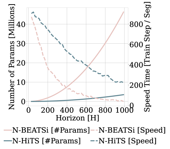
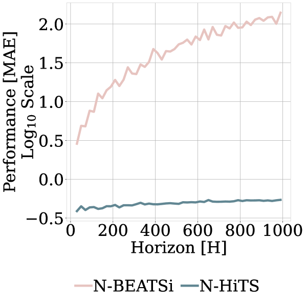
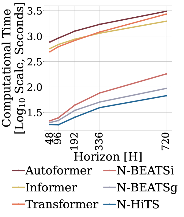
Despite all the recent progress, long-horizon forecasting remains challenging for neural networks, because their unbounded expressiveness translates directly into excessive computational complexity and forecast volatility, both of which become especially pronounced in this context. For instance, both attention and fully connected layers scale quadratically in memory and computational cost with respect to the forecasting horizon length. Fig. 1 illustrates how forecasting errors and computation costs inflate dramatically with growing forecasting horizon in the case of the fully connected architecture electricity consumption predictions. Attention-based predictions show similar behavior.

Neural long-horizon forecasting research has mostly focused on attention efficiency making self-attention sparse (Child et al. 2019; Li et al. 2019; Zhou et al. 2020) or local (Li et al. 2019). In the same vain, attention has been cleverly redefined through locality-sensitive hashing (Kitaev, Łukasz Kaiser, and Levskaya 2020) or FFT (Wu et al. 2021). Although that research has led to incremental improvements in compute cost and accuracy, the silver bullet long-horizon forecasting solution is yet to be found. In this paper we make a bold step in this direction by developing a novel forecasting approach that cuts long-horizon compute cost by an order of magnitude while simultaneously offering 16% accuracy improvements on a large array of multi-variate forecasting datasets compared to existing state-of-the-art Transformer-based techniques. We redefine existing fully-connected N-BEATS architecture (Oreshkin et al. 2020) by enhancing its input decomposition via multi-rate data sampling and its output synthesizer via multi-scale interpolation. Our extensive experiments show the importance of the proposed novel architectural components and validate significant improvements in accuracy and computational complexity of the proposed algorithm.

Our contributions are summarized below:

1.

Multi-Rate Data Sampling: We incorporate sub-sampling layers in front of fully-connected blocks, significantly reducing the memory footprint and the amount of computation needed, while maintaining the ability to model long-range dependencies.
2.

Hierarchical Interpolation: We enforce smoothness of the multi-step predictions by reducing the dimensionality of neural network’s prediction and matching its time scale with that of the final output via multi-scale hierarchical interpolation. This novel technique is not unique to our proposed model, and can be incorporated in different architectures.
3.

N-HiTS architecture: A novel way of hierarchically synchronizing the rate of input sampling with the scale of output interpolation across blocks, which induces each block to specialize on forecasting its own frequency band of the time-series signal.
4.

State-of-the-art results on six large-scale benchmark datasets from the long-horizon forecasting literature: electricity transformer temperature, exchange rate, electricity consumption, San Francisco bay area highway traffic, weather and influenza-like illness.

The remainder of this paper is structured as follows. Section 2 reviews relevant literature, Section 3 introduces notation and describes the methodology, Sections 4 and 5 describe and analyze our empirical findings. Finally, Section 6 concludes the paper.

2 Related Work

Neural forecasting. Over the past few years, deep forecasting methods have become ubiquitous in industrial forecasting systems, with examples in optimal resource allocation and planning in transportation (Laptev et al. 2017), large e-commerce retail (Wen et al. 2017; Olivares et al. 2021b; Paria et al. 2021; Rangapuram et al. 2021), or financial trading (Banushev and Barclay 2021). The evident success of the methods in recent forecasting competitions (Makridakis, Spiliotis, and Assimakopoulos 2020, 2021) has renovated the interest within the academic community (Benidis et al. 2020). In the context of multi-variate long-horizon forecasting, Transformer-based approaches have dominated the landscape in the recent years, including Autoformer (Wu et al. 2021), an encoder-decoder model with decomposition capabilities and an approximation to attention based on Fourier transform, Informer (Zhou et al. 2020), Transformer with MLP based multi-step prediction strategy, that approximates self-attention with sparsity, Reformer (Kitaev, Łukasz Kaiser, and Levskaya 2020), Transformer that approximates attention with locality-sensitive hashing and LogTrans (Li et al. 2019), Transformer with local/log-sparse attention.

Multi-step forecasting. Investigations of the bias/variance trade-off in multi-step forecasting strategies reveal that the direct strategy, which allocates a different model for each step, has low bias and high variance, avoiding error accumulation across steps, exhibited by the classical recursive strategy, but losing in terms of net model parsimony. Conversely, in the joint forecasting strategy, a single model produces forecasts for all steps in one shot, striking the perfect balance between variance and bias, avoiding error accumulation and leveraging shared model parameters (Bao, Xiong, and Hu 2014; Atiya and Taieb 2016; Wen et al. 2017).

Multi-rate input sampling. Previous forecasting literature recognized challenges of extremely long horizon predictions, and proposed mixed data sampling regression (MIDAS; Ghysels, Sinko, and Valkanov 2007; Armesto, Engemann, and Owyang 2010) to ameliorate the problem of parameter proliferation while preserving high frequency temporal information. MIDAS regressions maintained the classic recursive forecasting strategy of linear auto-regressive models, but defined a parsimonious fashion of feeding the inputs.

Interpolation. Interpolation has been extensively used to augment the resolution of modeled signals in many fields such as signal and image processing (Meijering 2002). In time-series forecasting, its applications range from completing unevenly sampled data and noise filters (Chow and loh Lin 1971; Fernandez 1981; Shukla and Marlin 2019; Rubanova, Chen, and Duvenaud 2019) to fine-grained quantile-regressions with recurrent networks (Gasthaus et al. 2019). To our knowledge, temporal interpolation has not been used to induce multi-scale hierarchical time-series forecasts.

3 N-HiTS Methodology

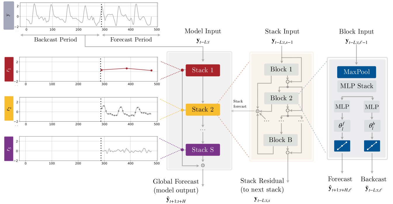
In this section, we describe our proposed approach, N-HiTS, whose high-level diagram and main principles of operation are depicted in Fig. 2. Our method extends the Neural Basis Expansion Analysis approach (N-BEATS; Oreshkin et al. 2020) in several important respects, making it more accurate and computationally efficient, especially in the context of long-horizon forecasting. In essence, our approach uses multi-rate sampling of the input signal and multi-scale synthesis of the forecast, resulting in a hierarchical construction of forecast, greatly reducing computational requirements and improving forecasting accuracy.

Similarly to N-BEATS, N-HiTS performs local nonlinear projections onto basis functions across multiple blocks. Each block consists of a multilayer perceptron (MLP), which learns to produce coefficients for the backcast and forecast outputs of its basis. The backcast output is used to clean the inputs of subsequent blocks, while the forecasts are summed to compose the final prediction. The blocks are grouped in stacks, each specialized in learning a different characteristic of the data using a different set of basis functions. The overall network input, $\mathbf{y}_{t-L:t}$ , consists of $L$ lags.

N-HiTS is composed of $S$ stacks, $B$ blocks each. Each block contains an MLP predicting forward and backward basis coefficients. The next subsections describe the novel components of our architecture. Note that in the following, we skip the stack index $s$ for brevity.

Multi-Rate Signal Sampling

At the input to each block $\ell$ , we propose to use a MaxPool layer with kernel size $k_{\ell}$ to help it focus on analyzing components of its input with a specific scale. Larger $k_{\ell}$ will tend to cut more high-frequency/small-time-scale components from the input of the MLP, forcing the block to focus on analyzing large scale/low frequency content. We call this multi-rate signal sampling, referring to the fact that the MLP in each block faces a different effective input signal sampling rate. Intuitively, this helps the blocks with larger pooling kernel size $k_{\ell}$ focus on analyzing large scale components critical for producing consistent long-horizon forecasts.

Additionally, multi-rate processing reduces the width of the MLP input for most blocks, limiting the memory footprint and the amount of computation as well as reducing the number of learnable parameters and hence alleviating the effects of overfitting, while maintaining the original receptive field. Given block $\ell$ input $\mathbf{y}_{t-L:t,\ell}$ (the input to the first block $\ell=1$ is the network-wide input, $\mathbf{y}_{t-L:t,1}\equiv\mathbf{y}_{t-L:t}$ ), this operation can be formalized as follows:

\mathbf{y}^{(p)}_{t-L:t,\ell}=\mathbf{MaxPool}\left(\mathbf{y}_{t-L:t,\ell},\;k_{\ell}\right)

(1)

Non-Linear Regression

Following subsampling, block $\ell$ looks at its input and non-linearly regresses forward $\mathbf{\theta}^{f}_{\ell}$ and backward $\mathbf{\theta}^{b}_{\ell}$ interpolation MLP coefficients that learns hidden vector $\mathbf{h}_{\ell}\in\mathbb{R}^{N_{h}}$ , which is then linearly projected:

\displaystyle\begin{split}\mathbf{h}_{\ell}&=\mathbf{MLP}_{\ell}\left(\mathbf{y}^{(p)}_{t-L:t,\ell}\right)\\ \boldsymbol{\theta}^{f}_{\ell}&=\textbf{LINEAR}^{f}\left(\mathbf{h}_{\ell}\right)\\ \boldsymbol{\theta}^{b}_{\ell}&=\textbf{LINEAR}^{b}\left(\mathbf{h}_{\ell}\right)\end{split}

(2)

The coefficients are then used to synthesize backcast $\mathbf{\tilde{y}}_{t-L:t,\ell}$ and forecast $\mathbf{\hat{y}}_{t+1:t+H,\ell}$ outputs of the block, via the process described below.

Hierarchical Interpolation

In most multi-horizon forecasting models, the cardinality of the neural network prediction equals the dimensionality of horizon, $H$ . For example, in N-BEATSi $|\boldsymbol{\theta}^{f}_{\ell}|=H$ ; in Transformer-based models, decoder attention layer cross-correlates $H$ output embeddings with $L$ encoded input embeddings ( $L$ tends to grow with growing $H$ ). This leads to quick inflation in compute requirements and unnecessary explosion in model expressiveness as horizon $H$ increases.

To combat these issues, we propose to use temporal interpolation. We define the dimensionality of the interpolation coefficients in terms of the expressiveness ratio $r_{\ell}$ that controls the number of parameters per unit of output time, $|\boldsymbol{\theta}^{f}_{\ell}|=\lceil r_{\ell}\,H\rceil$ . To recover the original sampling rate and predict all $H$ points in the horizon, we use temporal interpolation via the interpolation function $g$ :

\displaystyle\begin{split}\hat{y}_{\tau,\ell}&=g(\tau,\boldsymbol{\theta}^{f}_{\ell}),\quad\forall\tau\in\{t+1,\dots,t+H\},\\ \tilde{y}_{\tau,\ell}&=g(\tau,\boldsymbol{\theta}^{b}_{\ell}),\quad\forall\tau\in\{t-L,\dots,t\}.\end{split}

(3)

Interpolation can vary in smoothness, $g\in\mathcal{C}^{0},\mathcal{C}^{1},\mathcal{C}^{2}$ . In Appendix G we explore the nearest neighbor, piece-wise linear and cubic alternatives. For concreteness, the linear interpolator $g\in\mathcal{C}^{1}$ , along with the time partition $\mathcal{T}=\{t+1,t+1+1/r_{\ell},\ldots,t+H-1/r_{\ell},t+H\}$ , is defined as

\displaystyle\begin{split}g(\tau,\theta)&=\theta[t_{1}]+\left(\frac{\theta[t_{2}]-\theta[t_{1}]}{t_{2}-t_{1}}\right)(\tau-t_{1})\\ t_{1}&=\arg\min_{t\in\mathcal{T}:t\leq\tau}\tau-t,\quad t_{2}=t_{1}+1/r_{\ell}.\end{split}

(4)

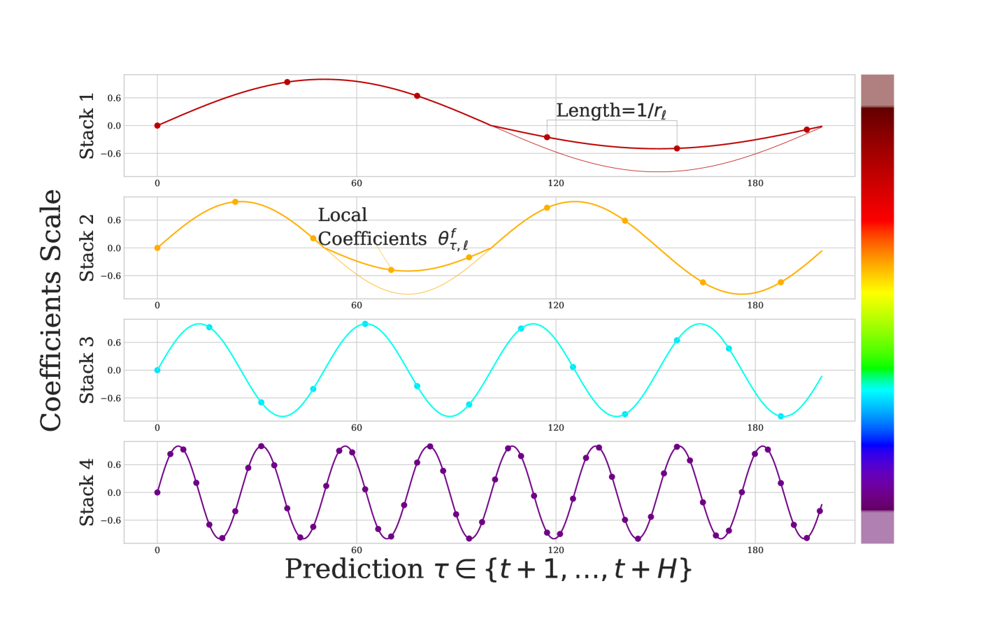
The hierarchical interpolation principle is implemented by distributing expressiveness ratios across blocks in a manner synchronized with multi-rate sampling. Blocks closer to the input have smaller $r_{\ell}$ and larger $k_{\ell}$ , implying that input blocks generate low-granularity signals via more aggressive interpolation, being also forced to look at more aggressively sub-sampled (and smoothed) signals. The resulting hierarchical forecast $\mathbf{\hat{y}}_{t+1:t+H}$ is assembled by summing the outputs of all blocks, essentially composing it out of interpolations at different time-scale hierarchy levels.

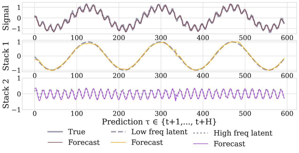
Since each block specializes on its own scale of input and output signal, this induces a clearly structured hierarchy of interpolation granularity, the intuition conveyed in Fig. 1 and 3. We propose to use exponentially increasing expressiveness ratios to handle a wide range of frequency bands while controlling the number of parameters. Alternatively, each stack can specialize in modeling a different known cycle of the time-series (weekly, daily etc.) using a matching $r_{\ell}$ (see Table A.3). Finally, the backcast residual formed at previous hierarchy scale is subtracted from the input of the next hierarchy level to amplify the focus of the next level block on signals outside of the band that has already been handled by the previous hierarchy members.

\begin{split}\mathbf{\hat{y}}_{t+1:t+H}&=\sum^{L}_{l=1}\hat{\mathbf{y}}_{t+1:t+H,\ell}\\ \mathbf{y}_{t-L:t,\ell+1}&=\mathbf{y}_{t-L:t,\ell}-\mathbf{\tilde{y}}_{t-L:t,\ell}\end{split}

Hierarchical interpolation has advantageous theoretical guarantees. We show in Appendix A, that it can approximate infinitely/dense horizons. As long as the interpolating function $g$ is characterized by projections to informed multi-resolution functions $V_{w}$ , and the forecast relationships are smooth.

Neural Basis Approximation Theorem. Let a forecast mapping be $\mathcal{Y}(\cdot\;|\;\mathbf{y}_{t-L:t}):[0,1]^{L}\rightarrow\mathcal{F}$ , where the forecast functions $\mathcal{F}=\{\mathcal{Y}(\tau):[0,1]\to\mathbb{R}\}=\mathcal{L}^{2}([0,1])$ representing a infinite/dense horizon, are square integrable. If the multi-resolution functions $V_{w}=\{\phi_{w,h}(\tau)=\phi(2^{w}(\tau-h))\;|\;w\in{\mathbb{Z}},h\in 2^{-w}\times[0,\dots,2^{w}]\}$ can arbitrarily approximate $\mathcal{L}^{2}([0,1])$ . And the projection $\mathrm{Proj}_{V_{w}}(\mathcal{Y}(\tau))$ varies smoothly on $\mathbf{y}_{t-L:t}$ . Then the forecast mapping $\mathcal{Y}(\cdot\;|\;\mathbf{y}_{t-L:t})$ can be arbitrarily approximated by a neural basis expansion learning a finite number of multi-resolution coefficients $\hat{\theta}_{w,h}$ . That is $\forall\epsilon>0$ ,

\int|\mathcal{Y}(\tau\;|\;\mathbf{y}_{t-L:t})-\sum_{w,h}\hat{\theta}_{w,h}(\mathbf{y}_{t-L:t})\phi_{w,h}(\tau)|d\tau\leq\epsilon

(5)

Examples of multi-resolution functions $V_{w}=\{\phi_{w,h}(\tau)=\phi(2^{w}(\tau-h))\;|\;w\in{\mathbb{Z}},h\in 2^{-w}\times[0,\dots,2^{w}]\}$ include piece-wise constants, piece-wise linear functions and splines with arbitrary approximation capabilities.

4 Experimental Results

We follow the experimental settings from (Wu et al. 2021; Zhou et al. 2020) (NeurIPS 2021 and AAAI 2021 Best Paper Award). We first describe datasets, baselines and metrics used for the quantitative evaluation of our model. Table 1 presents our key results, demonstrating SoTA performance of our method relative to existing work. We then carefully describe the details of training and evaluation setups. We conclude the section by describing ablation studies.

Table 1: Main empirical results in long-horizon forecasting setup, lower scores are better. Metrics are averaged over eight runs, best results are highlighted in bold. In Appendix E we complement the main results with standard deviations.

		N-HiTS (Ours)		N-BEATS		FEDformer		Autoformer		Informer		LogTrans		Reformer		DilRNN		ARIMA
	H.	MSE	MAE	MSE	MAE	MSE	MAE	MSE	MAE	MSE	MAE	MSE	MAE	MSE	MAE	MSE	MAE	MSE	MAE
ETTm₂	96	0.176	0.255	0.184	0.263	0.203	0.287	0.255	0.339	0.365	0.453	0.768	0.642	0.658	0.619	0.343	0.401	0.225	0.301
	192	0.245	0.305	0.273	0.337	0.269	0.328	0.281	0.340	0.533	0.563	0.989	0.757	1.078	0.827	0.424	0.468	0.298	0.345
	336	0.295	0.346	0.309	0.355	0.325	0.366	0.339	0.372	1.363	0.887	1.334	0.872	1.549	0.972	0.632	1.083	0.370	0.386
	720	0.401	0.413	0.411	0.425	0.421	0.415	0.422	0.419	3.379	1.388	3.048	1.328	2.631	1.242	0.634	0.594	0.478	0.445
ECL	96	0.147	0.249	0.145	0.247	0.183	0.297	0.201	0.317	0.274	0.368	0.258	0.357	0.312	0.402	0.233	0.927	1.220	0.814
	192	0.167	0.269	0.180	0.283	0.195	0.308	0.222	0.334	0.296	0.386	0.266	0.368	0.348	0.433	0.265	0.921	1.264	0.842
	336	0.186	0.290	0.200	0.308	0.212	0.313	0.231	0.338	0.300	0.394	0.280	0.380	0.350	0.433	0.235	0.896	1.311	0.866
	720	0.243	0.340	0.266	0.362	0.231	0.343	0.254	0.361	0.373	0.439	0.283	0.376	0.340	0.420	0.322	0.890	1.364	0.891
Exchange	96	0.092	0.202	0.098	0.206	0.139	0.276	0.197	0.323	0.847	0.752	0.968	0.812	1.065	0.829	0.383	0.45	0.296	0.214
	192	0.208	0.322	0.225	0.329	0.256	0.369	0.300	0.369	1.204	0.895	1.040	0.851	1.188	0.906	1.123	0.834	1.056	0.326
	336	0.301	0.403	0.493	0.482	0.426	0.464	0.509	0.524	1.672	1.036	1.659	1.081	1.357	0.976	1.612	1.051	2.298	0.467
	720	0.798	0.596	1.108	0.804	1.090	0.800	1.447	0.941	2.478	1.310	1.941	1.127	1.510	1.016	1.827	1.131	20.666	0.864
TrafficL	96	0.402	0.282	0.398	0.282	0.562	0.349	0.613	0.388	0.719	0.391	0.684	0.384	0.732	0.423	0.580	0.308	1.997	0.924
	192	0.420	0.297	0.409	0.293	0.562	0.346	0.616	0.382	0.696	0.379	0.685	0.390	0.733	0.420	0.739	0.383	2.044	0.944
	336	0.448	0.313	0.449	0.318	0.570	0.323	0.622	0.337	0.777	0.420	0.733	0.408	0.742	0.420	0.804	0.419	2.096	0.960
	720	0.539	0.353	0.589	0.391	0.596	0.368	0.660	0.408	0.864	0.472	0.717	0.396	0.755	0.423	0.695	0.372	2.138	0.971
Weather	96	0.158	0.195	0.167	0.203	0.217	0.296	0.266	0.336	0.300	0.384	0.458	0.490	0.689	0.596	0.193	0.245	0.217	0.258
	192	0.211	0.247	0.229	0.261	0.276	0.336	0.307	0.367	0.598	0.544	0.658	0.589	0.752	0.638	0.255	0.306	0.263	0.299
	336	0.274	0.300	0.287	0.304	0.339	0.380	0.359	0.395	0.578	0.523	0.797	0.652	0.064	0.596	0.329	0.360	0.330	0.347
	720	0.351	0.353	0.368	0.359	0.403	0.428	0.419	0.428	1.059	0.741	0.869	0.675	1.130	0.792	0.521	0.495	0.425	0.405
ILI	24	1.862	0.869	1.879	0.886	2.203	0.963	3.483	1.287	5.764	1.677	4.480	1.444	4.400	1.382	4.538	1.449	5.554	1.434
	36	2.071	0.934	2.210	1.018	2.272	0.976	3.103	1.148	4.755	1.467	4.799	1.467	4.783	1.448	3.709	1.273	6.940	1.676
	48	2.134	0.932	2.440	1.088	2.209	0.981	2.669	1.085	4.763	1.469	4.800	1.468	4.832	1.465	3.436	1.238	7.192	1.736
	60	2.137	0.968	2.547	1.057	2.545	1.061	2.770	1.125	5.264	1.564	5.278	1.560	4.882	1.483	3.703	1.272	6.648	1.656

Datasets

All large-scale datasets used in our empirical studies are publicly available and have been used in neural forecasting literature, particularly in the context of long-horizon (Lai et al. 2017; Zhou et al. 2019; Li et al. 2019; Wu et al. 2021). Table A1 summarizes their characteristics. Each set is normalized with the train data mean and standard deviation.

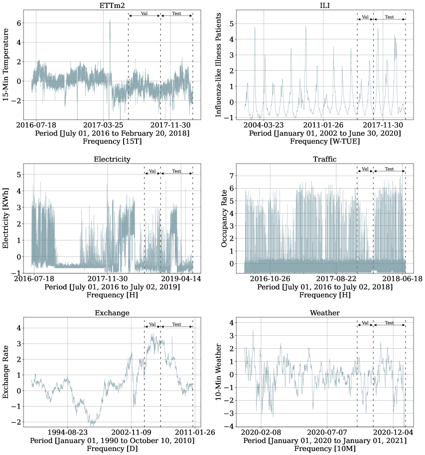
Electricity Transformer Temperature. The ETTm₂ dataset measures an electricity transformer from a region of a province of China including oil temperature and variants of load (such as high useful load and high useless load) from July 2016 to July 2018 at a fifteen minutes frequency. Exchange-Rate. The Exchange dataset is a collection of daily exchange rates of eight countries relative to the US dollar. The countries include Australia, UK, Canada, Switzerland, China, Japan, New Zealand and Singapore from 1990 to 2016. Electricity. The ECL dataset reports the fifteen minute electricity consumption (KWh) of 321 customers from 2012 to 2014. For comparability, we aggregate it hourly. San Francisco Bay Area Highway Traffic. This TrafficL dataset was collected by the California Department of Transportation, it reports road hourly occupancy rates of 862 sensors, from January 2015 to December 2016. Weather. This Weather dataset contains the 2020 year of 21 meteorological measurements recorded every 10 minutes from the Weather Station of the Max Planck Biogeochemistry Institute in Jena, Germany. Influenza-like illness. The ILI dataset reports weekly recorded influenza-like illness (ILI) patients from Centers for Disease Control and Prevention of the United States from 2002 to 2021. It is a ratio of ILI patients vs. the week’s total.

Evaluation Setup

We evaluate the accuracy of our approach using mean absolute error (MAE) and mean squared error (MSE) metrics, which are well-established in the literature (Zhou et al. 2020; Wu et al. 2021), for varying horizon lengths $H$ :

\mathrm{MSE}=\frac{1}{H}\sum^{t+H}_{\tau=t}\left(\mathbf{y}_{\tau}-\hat{\mathbf{y}}_{\tau}\right)^{2},\qquad\mathrm{MAE}=\frac{1}{H}\sum^{t+H}_{\tau=t}|\mathbf{y}_{\tau}-\hat{\mathbf{y}}_{\tau}|

(6)

Note that for multivariate datasets, our algorithm produces forecast for each feature in the dataset and metrics are averaged across dataset features. Since our model is univariate, each variable is predicted using only its own history, $\mathbf{y}_{t-L:t}$ , as input. Datasets are partitioned into train, validation and test splits. Train split is used to train model parameters, validation split is used to tune hyperparameters, and test split is used to compute metrics reported in Table 1. Appendix 4 shows partitioning into train, validation and test splits: seventy, ten, and twenty percent of the available observations respectively, with the exception of ETTm₂ that uses twenty percent as validation.

Key Results

We compare N-HiTS to the following SoTA multivariate baselines: (1) FEDformer (Zhou et al. 2022), (2) Autoformer (Wu et al. 2021), (3) Informer (Zhou et al. 2020), (4) Reformer (Kitaev, Łukasz Kaiser, and Levskaya 2020) and (5) LogTrans (Li et al. 2019). Additionally, we consider the univariate baselines: (6) DilRNN (Chang et al. 2017) and (7) auto-ARIMA (Hyndman and Khandakar 2008).

Forecasting Accuracy. Table 1 summarizes the multivariate forecasting results. N-HiTS outperforms the best baseline, with average relative error decrease across datasets and horizons of 14% in MAE and 16% in MSE. N-HiTS maintains a comparable performance to other state-of-the-art methods for the shortest measured horizon (96/24), while for the longest measured horizon (720/60) decreases multivariate MAE by 11% and MSE by 17%. We complement the key results in Table 1, with the additional univariate forecasting experiments in Appendix F, again demonstrating state-of-the-art performance against baselines.

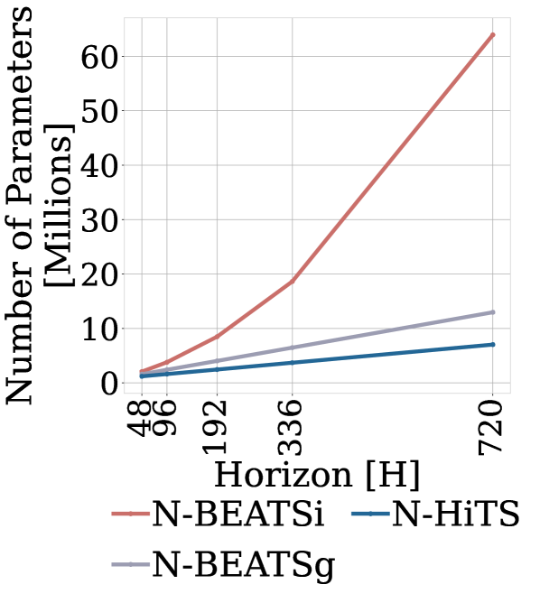
Computational Efficiency. We measure the computational training time of N-HiTS, N-BEATS and Transformer-based methods in the multivariate setting and show compare in Figure 4. The experiment monitors the whole training process for the ETTm₂ dataset. For the Transformer-based models we used hyperparameters reported in (Wu et al. 2021). Compared to the Transformer-based methods, N-HiTS is 45 $\times$ faster than Autoformer. In terms of memory, N-HiTS has less than 26% of the parameters of the second-best alternative, since it scales linearly with respect to the input’s length. Compared to the original N-BEATS, our method is 1.26 $\times$ faster and requires only 54% of the parameters. Finally, while N-HiTS is an univariate model, it has global (shared) parameters for all time-series in the dataset. Just like (Oreshkin et al. 2020), our experiments (Appendix I) show that N-HiTS maintains constant parameter/training computational complexity regarding dataset’s size.

Training and Hyperparameter Optimization

We consider a minimal space of hyperparameters to explore configurations of the N-HiTS architecture. First, we consider the kernel pooling size for multi-rate sampling from Equation (1). Second, the number of coefficients from Equation (2) that we selected between several alternatives, some matching common seasonalities of the datasets and others exponentially increasing. We tune the random seed to escape underperforming local minima. Details are reported in Table A3 in Appendix D.

During the hyperparameter optimization phase, we measure MAE performance on the validation set and use a Bayesian optimization library (HYPEROPT; Bergstra et al. 2011), with 20 iterations. We use the optimal configuration based on the validation loss to make prediction on the test set. We refer to the combination of hyperparameter optimization and test prediction as a run. N-HiTS is implemented in PyTorch (Paszke et al. 2019) and trained using ADAM optimizer (Kingma and Ba 2014), MAE loss, batch size 256 and initial learning rate of 1e-3, halved three times across the training procedure. All our experiments are conducted on a GeForce RTX 2080 GPU.

Ablation Studies

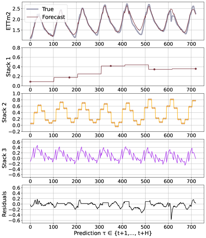
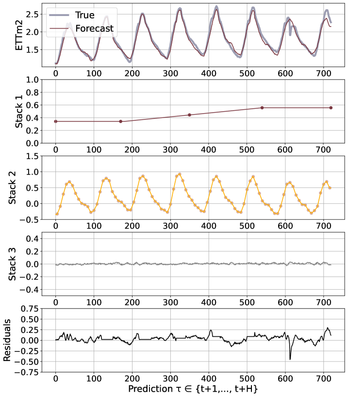
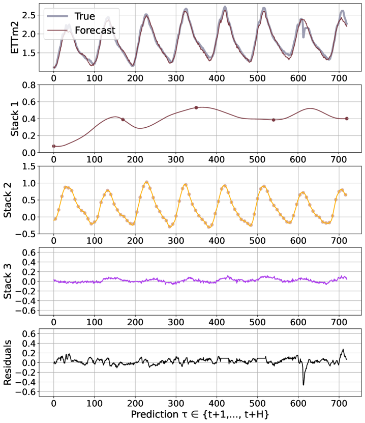
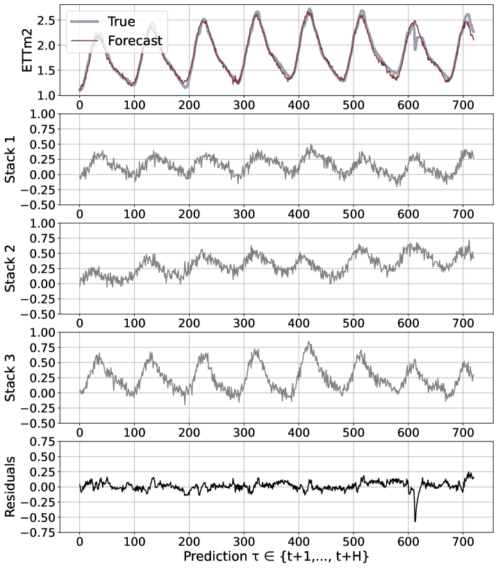
We believe that the advantages of the N-HiTS architecture are rooted in its multi-rate hierarchical nature. Fig. 5 shows a qualitative comparison of N-HiTS with and without hierarchical interpolation/multi-rate sampling components. We clearly see N-HiTS developing the ability to produce interpretable forecast decomposition providing valuable information about trends and seasonality in separate channels, unlike the control model. Appendix G presents the decomposition for the different interpolation techniques. We support our qualitative conclusion with quantitative results. We define the following set of alternative models: N-HiTS, our proposed model with both multi-rate sampling and hierarchical interpolation, N-HiTS₂ only hierarchical interpolation, N-HiTS₃ only multi-rate sampling, N-HiTS₄ no multi-rate sampling or interpolation (corresponds to the original N-BEATSg (Oreshkin et al. 2020)), finally N-BEATSi, the interpreatble version of the N-BEATS ((Oreshkin et al. 2020)). Tab. 2 clearly shows that the combination of both proposed components (hierarchical interpolation and multi-rate sampling) results in the best performance, emphasizing their complementary nature in long-horizon forecasting. We see that the original N-BEATS is consistently worse, especially the N-BEATSi. The advantages of the proposed techniques for long-horizon forecasting, multi-rate sampling and interpolation, are not limited to the N-HiTS architecture. In Appendix H we demonstrate how adding them to a DilRNN improve its performance.

Table 2: Empirical evaluation of long multi-horizon multivariate forecasts for N-HiTS with/without enhancements. MAE and MSE for predictions averaged over eight runs, and five datasets, the best result is highlighted in bold, second best in blue (lower is better).

		N-HiTS	N-HiTS₂	N-HiTS₃	N-HiTS₄	N-BEATSi
A. MSE	96	0.195	0.196	0.192	0.196	0.209
	192	0.250	0.261	0.251	0.263	0.266
	336	0.315	0.315	0.342	0.346	0.408
	720	0.484	0.498	0.518	0.548	0.794
A. MAE	96	0.239	0.241	0.237	0.240	0.254
	192	0.290	0.299	0.291	0.300	0.307
	336	0.338	0.342	0.346	0.352	0.405
	720	0.439	0.450	0.454	0.468	0.597

Additional ablation studies are reported in Appendix G. The MaxPool multi-rate sampling wins over AveragePool. Linear interpolation wins over nearest neighbor and cubic. Finally and most importantly, we show that the order in which hierarchical interpolation is implemented matters significantly. The best configuration is to have the low-frequency/large-scale components synthesized and removed from analysis first, followed by more fine-grained modeling of high-frequency/intermittent signals.

5 Discussion of Findings

Our results indicate the complementarity and effectiveness of multi-rate sampling and hierarchical interpolation for long-horizon time-series forecasting. Table 2 indicates that these components enforce a useful inductive bias compared to both the free-form model $\texttt{{N-HiTS}}_{4}$ (plain fully connected architecture) and the parametric model N-BEATSi (polynomial trend and sinusoidal seasonality used as basis functions in two respective stacks). The latter obviously providing a detrimental inductive bias for long-horizon forecasting. Notwithstanding our current success, we believe we barely scratched the surface in the right direction and further progress is possible using advanced multi-scale processing approaches in the context of time-series forecasting, motivating further research.

N-HiTS outperforms SoTA baselines while simultaneously providing an interpretable non-linear decomposition. Fig. 1 and 5 showcase N-HiTS perfectly specializing and reconstructing latent harmonic signals from synthetic and real data respectively. This novel interpretable decomposition can provide insights to users, improving their confidence in high-stakes applications like healthcare. Finally, N-HiTS hierarchical interpolation can be explored from the multi-resolution analysis perspective (Daubechies 1992). Replacing the sequential projections from the interpolation functions onto these Wavelet induced spaces is an interesting line of research.

Our study raises a question about the effectiveness of the existing long-horizon multi-variate forecasting approaches, as all of them are substantially outperformed by our univariate algorithm. If these approaches underperform due to problems with overfitting and model parsimony at the level of marginals, it is likely that the integration of our approach with Transformer-inspired architectures could form a promising research direction as the univariate results in Appendix F suggest. However, there is also a chance that the existing approaches underperform due to their inability to effectively integrate information from multiple variables, which clearly hints at possibly untapped research potential in this area. Whichever is the case, we believe our results provide a strong guidance signal and a valuable baseline for future research in the area of long-horizon multi-variate forecasting.

6 Conclusions

We proposed a novel neural forecasting algorithm N-HiTS that combines two complementary techniques, multi-rate input sampling and hierarchical interpolation, to produce drastically improved, interpretable and computationally efficient long-horizon time-series predictions. Our model, operating in the univariate regime and accepting only the predicted time-series’ history, significantly outperforms all previous Transformer-based multi-variate models using an order of magnitude less computation. This sets a new baseline for all ensuing multi-variate work on six popular datasets and motivates further research to effectively use information from multiple variables.

Acknowledgements

This work was partially supported by the Defense Advanced Research Projects Agency (award FA8750-17-2-0130), the National Science Foundation (grant 2038612), the Space Technology Research Institutes grant from NASA’s Space Technology Research Grants Program, the U.S. Department of Homeland Security (award 18DN-ARI-00031), and by the U.S. Army Contracting Command (contracts W911NF20D0002 and W911NF22F0014 delivery order #4). Thanks to Mengfei Cao for in-depth discussion and comments on the method, and Kartik Gupta for his insights on the connection of N-HiTS with Wavelet’s theory. The authors are also grateful to Stefania La Vattiata for her assistance in the upbeat visualization of the Neural Hierarchical Interpolation for Time Series method.

References

Alaa and van der Schaar (2019) Alaa, A. M.; and van der Schaar, M. 2019. Attentive State-Space Modeling of Disease Progression. In Wallach, H.; Larochelle, H.; Beygelzimer, A.; d'Alché-Buc, F.; Fox, E.; and Garnett, R., eds., 33rd Conference on Neural Information Processing Systems (NeurIPS 2019), volume 32. Curran Associates, Inc.
Armesto, Engemann, and Owyang (2010) Armesto, M. T.; Engemann, K. M.; and Owyang, M. T. 2010. Forecasting with Mixed Frequencies. Federal Reserve Bank of St. Louis Review, 92: 521–536.
Atiya and Taieb (2016) Atiya, A.; and Taieb, B. 2016. A Bias and Variance Analysis for Multistep-Ahead Time Series Forecasting. IEEE transactions on neural networks and learning systems, 27(1): 2162–2388.
Banushev and Barclay (2021) Banushev, B.; and Barclay, R. 2021. Enhancing trading strategies through cloud services and machine learning.
Bao, Xiong, and Hu (2014) Bao, Y.; Xiong, T.; and Hu, Z. 2014. Multi-step-ahead time series prediction using multiple-output support vector regression. Neurocomputing, 129: 482–493.
Barron (1993) Barron, A. R. 1993. Universal approximation bounds for superpositions of a sigmoidal function. IEEE Transactions on Information theory, 39(3): 930–945.
Basher (2006) Basher, R. 2006. Global early warning systems for natural hazards: Systematic and people-centred. Philosophical transactions. Series A, Mathematical, physical, and engineering sciences, 364: 2167–82.
Bengio, Courville, and Vincent (2012) Bengio, Y.; Courville, A. C.; and Vincent, P. 2012. Unsupervised Feature Learning and Deep Learning: A Review and New Perspectives. CoRR, abs/1206.5538.
Benidis et al. (2020) Benidis, K.; Rangapuram, S. S.; Flunkert, V.; Wang, B.; Maddix, D.; Turkmen, C.; Gasthaus, J.; Bohlke-Schneider, M.; Salinas, D.; Stella, L.; Callot, L.; and Januschowski, T. 2020. Neural forecasting: Introduction and literature overview. Computing Research Repository.
Bergstra et al. (2011) Bergstra, J.; Bardenet, R.; Bengio, Y.; and Kégl, B. 2011. Algorithms for Hyper-Parameter Optimization. In Shawe-Taylor, J.; Zemel, R.; Bartlett, P.; Pereira, F.; and Weinberger, K. Q., eds., Advances in Neural Information Processing Systems, volume 24, 2546–2554. Curran Associates, Inc.
Boggess and Narcowich (2015) Boggess, A.; and Narcowich, F. J. 2015. A first course in wavelets with Fourier analysis. John Wiley & Sons.
Chang et al. (2017) Chang, S.; Zhang, Y.; Han, W.; Yu, M.; Guo, X.; Tan, W.; Cui, X.; Witbrock, M.; Hasegawa-Johnson, M. A.; and Huang, T. S. 2017. Dilated Recurrent Neural Networks. In Guyon, I.; Luxburg, U. V.; Bengio, S.; Wallach, H.; Fergus, R.; Vishwanathan, S.; and Garnett, R., eds., Advances in Neural Information Processing Systems, volume 30. Curran Associates, Inc.
Child et al. (2019) Child, R.; Gray, S.; Radford, A.; and Sutskever, I. 2019. Generating Long Sequences with Sparse Transformers. CoRR, abs/1904.10509.
Chow and loh Lin (1971) Chow, G. C.; and loh Lin, A. 1971. Best Linear Unbiased Interpolation, Distribution, and Extrapolation of Time Series by Related Series. The Review of Economics and Statistics, 53(4): 372–375.
Churpek, Adhikari, and Edelson (2016) Churpek, M. M.; Adhikari, R.; and Edelson, D. P. 2016. The value of vital sign trends for detecting clinical deterioration on the wards. Resuscitation, 102: 1–5.
Daubechies (1992) Daubechies, I. 1992. Ten lectures on wavelets. SIAM.
Du, Su, and Wei (2022) Du, D.; Su, B.; and Wei, Z. 2022. Preformer: Predictive Transformer with Multi-Scale Segment-wise Correlations for Long-Term Time Series Forecasting. Computing Research Repository, abs/2202.11356.
Fan et al. (2019) Fan, C.; Zhang, Y.; Pan, Y.; Li, X.; Zhang, C.; Yuan, R.; Wu, D.; Wang, W.; Pei, J.; and Huang, H. 2019. Multi-Horizon Time Series Forecasting with Temporal Attention Learning. In Proceedings of the 25th ACM SIGKDD International Conference on Knowledge Discovery & Data Mining, KDD ’19, 2527–2535. New York, NY, USA: Association for Computing Machinery. ISBN 9781450362016.
Fernandez (1981) Fernandez, R. B. 1981. A Methodological Note on the Estimation of Time Series. The Review of Economics and Statistics, 63(3): 471–476.
Field et al. (2012) Field, C. B.; Barros, V.; Stocker, T. F.; and Dahe, Q. 2012. Managing the risks of extreme events and disasters to advance climate change adaptation: special report of the intergovernmental panel on climate change. Cambridge University Press.
Gasthaus et al. (2019) Gasthaus, J.; Benidis, K.; Wang, B.; Rangapuram, S. S.; Salinas, D.; Flunkert, V.; and Januschowski, T. 2019. Probabilistic Forecasting with Spline Quantile Function RNNs. In AISTATS.
Ghysels, Sinko, and Valkanov (2007) Ghysels, E.; Sinko, A.; and Valkanov, R. 2007. MIDAS Regressions: Further Results and New Directions. Econometric Reviews, 26(1): 53–90.
Hanin and Sellke (2017) Hanin, B.; and Sellke, M. 2017. Approximating Continuous Functions by ReLU Nets of Minimal Width.
Hornik (1991) Hornik, K. 1991. Approximation capabilities of multilayer feedforward networks. Neural Networks, 4(2): 251–257.
Hyndman and Fan (2009) Hyndman, R. J.; and Fan, S. 2009. Density forecasting for long-term peak electricity demand. IEEE Transactions on Power Systems, 25(2): 1142–1153.
Hyndman and Khandakar (2008) Hyndman, R. J.; and Khandakar, Y. 2008. Automatic Time Series Forecasting: The forecast Package for R. Journal of Statistical Software, Articles, 27(3): 1–22.
Kingma and Ba (2014) Kingma, D. P.; and Ba, J. 2014. ADAM: A Method for Stochastic Optimization. Cite arxiv:1412.6980Comment: Published as a conference paper at the 3rd International Conference for Learning Representations (ICLR), San Diego, 2015.
Kitaev, Łukasz Kaiser, and Levskaya (2020) Kitaev, N.; Łukasz Kaiser; and Levskaya, A. 2020. Reformer: The Efficient Transformer. In 8th International Conference on Learning Representations, (ICLR 2020).
Lai et al. (2017) Lai, G.; Chang, W.; Yang, Y.; and Liu, H. 2017. Modeling Long- and Short-Term Temporal Patterns with Deep Neural Networks. Special Interest Group on Information Retrieval Conference 2018 (SIGIR 2018), abs/1703.07015.
Laptev et al. (2017) Laptev, N.; Yosinsk, J.; Erran, L. L.; and Smyl, S. 2017. Time-series extreme event forecasting with neural networks at UBER. In 34th International Conference on Machine Learning ICML 2017, Time Series Workshop.
Li et al. (2019) Li, S.; Jin, X.; Xuan, Y.; Zhou, X.; Chen, W.; Wang, Y.; and Yan, X. 2019. Enhancing the Locality and Breaking the Memory Bottleneck of Transformer on Time Series Forecasting. In Wallach, H.; Larochelle, H.; Beygelzimer, A.; d'Alché-Buc, F.; Fox, E.; and Garnett, R., eds., 33rd Conference on Neural Information Processing Systems (NeurIPS 2019), volume 32. Curran Associates, Inc.
Lim et al. (2021) Lim, B.; Arık, S. Ö.; Loeff, N.; and Pfister, T. 2021. Temporal Fusion Transformers for interpretable multi-horizon time series forecasting. International Journal of Forecasting.
Makridakis, Spiliotis, and Assimakopoulos (2020) Makridakis, S.; Spiliotis, E.; and Assimakopoulos, V. 2020. The M4 Competition: 100,000 time series and 61 forecasting methods. International Journal of Forecasting, 36(1): 54–74. M4 Competition.
Makridakis, Spiliotis, and Assimakopoulos (2021) Makridakis, S.; Spiliotis, E.; and Assimakopoulos, V. 2021. Predicting/hypothesizing the findings of the M5 competition. International Journal of Forecasting.
Marcellino, Stock, and Watson (2006) Marcellino, M.; Stock, J. H.; and Watson, M. W. 2006. A comparison of direct and iterated multistep AR methods for forecasting macroeconomic time series. Journal of Econometrics, 135(1): 499–526.
Meijering (2002) Meijering, E. 2002. A chronology of interpolation: from ancient astronomy to modern signal and image processing. Proceedings of the IEEE, 90(3): 319–342.
Olivares et al. (2021a) Olivares, K. G.; Challu, C.; Marcjasz, G.; Weron, R.; and Dubrawski, A. 2021a. Neural basis expansion analysis with exogenous variables: Forecasting electricity prices with NBEATSx. International Journal of Forecasting, submitted, Working Paper version available at arXiv:2104.05522.
Olivares et al. (2021b) Olivares, K. G.; Meetei, N. O.; Ma, R.; Reddy, R.; Cao, M.; and Dicker, L. 2021b. Probabilistic Hierarchical Forecasting with Deep Poisson Mixtures. International Journal of Forecasting (Hierarchical Forecasting special issue), submitted, Working Paper version available at arXiv:2110.13179.
Oreshkin et al. (2020) Oreshkin, B. N.; Carpov, D.; Chapados, N.; and Bengio, Y. 2020. N-BEATS: Neural basis expansion analysis for interpretable time series forecasting. In 8th International Conference on Learning Representations, ICLR 2020.
Paria et al. (2021) Paria, B.; Sen, R.; Ahmed, A.; and Das, A. 2021. Hierarchically Regularized Deep Forecasting. In Submitted to Proceedings of the 39th International Conference on Machine Learning. PMLR. Working Paper version available at arXiv:2106.07630.
Paszke et al. (2019) Paszke et al. 2019. PyTorch: An Imperative Style, High-Performance Deep Learning Library. In Wallach, H.; Larochelle, H.; Beygelzimer, A.; d Alché-Buc, F.; Fox, E.; and Garnett, R., eds., Advances in Neural Information Processing Systems 32, 8024–8035. Curran Associates, Inc.
Rangapuram et al. (2021) Rangapuram, S. S.; Werner, L. D.; Benidis, K.; Mercado, P.; Gasthaus, J.; and Januschowski, T. 2021. End-to-End Learning of Coherent Probabilistic Forecasts for Hierarchical Time Series. In Balcan, M. F.; and Meila, M., eds., Proceedings of the 38th International Conference on Machine Learning, Proceedings of Machine Learning Research. PMLR.
Rubanova, Chen, and Duvenaud (2019) Rubanova, Y.; Chen, R. T. Q.; and Duvenaud, D. 2019. Latent ODEs for Irregularly-Sampled Time Series. In Advances in Neural Information Processing Systems 33 (NeurIPS 2019).
Salinas et al. (2020) Salinas, D.; Flunkert, V.; Gasthaus, J.; and Januschowski, T. 2020. DeepAR: Probabilistic forecasting with autoregressive recurrent networks. International Journal of Forecasting, 36(3): 1181–1191.
Shukla and Marlin (2019) Shukla, S. N.; and Marlin, B. M. 2019. Interpolation-Prediction Networks for Irregularly Sampled Time Series. Cite arxiv:1412.6980Comment: Published as a conference paper at the 7th International Conference for Learning Representations (ICLR), New Orleans, 2019.
Taylor and Letham (2018) Taylor, S. J.; and Letham, B. 2018. Forecasting at scale. The American Statistician, 72(1): 37–45.
Wen et al. (2017) Wen, R.; Torkkola, K.; Narayanaswamy, B.; and Madeka, D. 2017. A Multi-Horizon Quantile Recurrent Forecaster. In 31st Conference on Neural Information Processing Systems NIPS 2017, Time Series Workshop.
Woo et al. (2022) Woo, G.; Liu, C.; Sahoo, D.; Kumar, A.; and Hoi, S. C. H. 2022. ETSformer: Exponential Smoothing Transformers for Time-series Forecasting. Computing Research Repository, abs/2202.01381.
Wu et al. (2021) Wu, H.; Xu, J.; Wang, J.; and Long, M. 2021. Autoformer: Decomposition Transformers with Auto-Correlation for Long-Term Series Forecasting. In Ranzato, M.; Beygelzime, A.; Liang, P.; Vaughan, J.; and Dauphin, Y., eds., Advances in Neural Information Processing Systems 35 (NeurIPS 2021).
Zhou et al. (2020) Zhou, H.; Zhang, S.; Peng, J.; Zhang, S.; Li, J.; Xiong, H.; and Zhang, W. 2020. Informer: Beyond Efficient Transformer for Long Sequence Time-Series Forecasting. The Association for the Advancement of Artificial Intelligence Conference 2021 (AAAI 2021)., abs/2012.07436.
Zhou et al. (2019) Zhou, S.; Zhou, L.; Mao, M.; Tai, H.; and Wan, Y. 2019. An Optimized Heterogeneous Structure LSTM Network for Electricity Price Forecasting. IEEE Access, 7: 108161–108173.
Zhou et al. (2022) Zhou, T.; Ma, Z.; Wen, Q.; Wang, X.; Sun, L.; and Jin, R. 2022. FEDformer: Frequency Enhanced Decomposed Transformer for Long-term Series Forecasting. Computing Research Repository, abs/2201.12740.
Ziel and Steinert (2018) Ziel, F.; and Steinert, R. 2018. Probabilistic mid- and long-term electricity price forecasting. Renewable and Sustainable Energy Reviews, 94: 251–266.

Appendix A Neural Basis Approximation Theorem

In this Appendix we prove the neural basis expansion approximation theorem introduced in Section 4. We show that N-HiTS’ hierarchical interpolation can arbitrarily approximate infinitely long horizons ( $\tau\in[0,1]$ continuous horizon), as long as the interpolating functions $g$ are defined by a projections to informed multi-resolution functions, and the forecast relationships satisfy smoothness conditions. We prove the case when $g_{w,h}(\tau)=\theta_{w,h}\phi_{w,h}(\tau)=\theta_{w,h}\text{1}\{\tau\in[2^{-w}(h-1),2^{-w}h]\}$ are piecewise constants and the inputs $\mathbf{y}_{t-L:t}\in[0,1]$ . The proof for linear, spline functions and $\mathbf{y}_{t-L:t}\in[a,b]$ is analogous.

Lemma 1. Let a function representing an infinite forecast horizon be $\mathcal{Y}:[0,1]\rightarrow\mathbb{R}$ a square integrable function $\mathcal{L}^{2}([0,1])$ . The forecast function $\mathcal{Y}$ can be arbitrarily well approximated by a linear combination of piecewise constants:

V_{w}=\{\phi_{w,h}(\tau)=\phi(2^{w}(\tau-h))\;|\;w\in{\mathbb{Z}},h\in 2^{-w}\times[0,\dots,2^{w}]\}\quad

where $w\in\mathbb{N}$ controls the frequency/indicator’s length and $h$ the time-location (knots) around which the indicator $\phi_{w,h}(\tau)=\text{1}\{\tau\in[2^{-w}(h-1),2^{-w}h]\}$ is active. That is, $\forall\epsilon>0$ , there is a $w\in\mathbb{N}$ and $\hat{\mathcal{Y}}(\tau|\mathbf{y}_{t-L:t})=\mathrm{Proj}_{V_{w}}(\mathcal{Y}(\tau|\mathbf{y}_{t-L:t}))\in\mathrm{Span}(\phi_{w,h})$ such that

\int_{[0,1]}|\mathcal{Y}(\tau)-\hat{\mathcal{Y}}(\tau)|d\tau=\int_{[0,1]}|\mathcal{Y}(\tau)-\sum_{w,h}\theta_{w,h}\phi_{w,h}(\tau)|d\tau\leq\epsilon

(7)

Proof.

This classical proof can be traced back to Haar’s work (1910). The indicator functions $V_{w}=\{\phi_{w,h}(\tau)\}$ are also referred in literature as Haar scaling functions or father wavelets. Details provided in (Boggess and Narcowich 2015).Let the number of coefficients for the $\epsilon$ -approximation $\hat{\mathcal{Y}}(\tau|\mathbf{y}_{t-L:t})$ be denoted as $N_{\epsilon}=\sum^{w}_{i=0}2^{i}$ .

∎

Lemma 2. Let a forecast mapping $\mathcal{Y}(\cdot\;|\;\mathbf{y}_{t-L:t}):[0,1]^{L}\to\mathcal{L}^{2}([0,1])$ be $\epsilon$ -approximated by $\hat{\mathcal{Y}}(\tau|\mathbf{y}_{t-L:t})=\mathrm{Proj}_{V_{w}}(\mathcal{Y}(\tau|\mathbf{y}_{t-L:t}))$ , the projection to multi-resolution piecewise constants. If the relationship between $\mathbf{y}_{t-L:t}\in[0,1]^{L}$ and $\theta_{w,h}$ varies smoothly, for instance $\theta_{w,h}:[0,1]^{L}\to\mathbb{R}$ is a K-Lipschitz function then for all $\epsilon>0$ there exists a three-layer neural network $\hat{\theta}_{w,h}:[0,1]^{L}\rightarrow\mathbb{R}$ with $O\left(L\right(\frac{K}{\varepsilon}\left){}^{L}\right)$ neurons and $\mathrm{ReLU}$ activations such that

\int_{[0,1]^{L}}|\theta_{w,h}(\mathbf{y}_{t-L:t})-\hat{\theta}_{w,h}(\mathbf{y}_{t-L:t})|d\mathbf{y}_{t-L:t}\leq\epsilon

(8)

Proof.

This lemma is a special case of the neural universal approximation theorem that states the approximation capacity of neural networks of arbitrary width (Hornik 1991). The theorem has refined versions where the width can be decreased under more restrictive conditions for the approximated function (Barron 1993; Hanin and Sellke 2017). ∎

Theorem 1. Let a forecast mapping be

$\mathcal{Y}(\cdot\;|\;\mathbf{y}_{t-L:t}):[0,1]^{L}\rightarrow\mathcal{F}$ , where the forecast functions $\mathcal{F}=\{\mathcal{Y}(\tau):[0,1]\to\mathbb{R}\}=\mathcal{L}^{2}([0,1])$ representing a continuous horizon, are square integrable.

If the multi-resolution functions $V_{w}$ can arbitrarily approximate $\mathcal{L}^{2}([0,1])$ . And the projection $\mathrm{Proj}_{V_{w}}(\mathcal{Y}(\tau))$ varies smoothly on $\mathbf{y}_{t-L:t}$ . Then the forecast mapping $\mathcal{Y}(\cdot\;|\;\mathbf{y}_{t-L:t})$ can be arbitrarily approximated by a neural network learning a finite number of multi-resolution coefficients $\hat{\theta}_{w,h}$ .

That is $\forall\epsilon>0$ ,

\displaystyle\begin{split}\int|\mathcal{Y}(\tau\;|\;\mathbf{y}_{t-L:t})-\tilde{\mathcal{Y}}(\tau\;|\;\mathbf{y}_{t-L:t})|d\tau\qquad\qquad\qquad\qquad\qquad\\ =\int|\mathcal{Y}(\tau\;|\;\mathbf{y}_{t-L:t})-\sum_{w,h}\hat{\theta}_{w,h}(\mathbf{y}_{t-L:t})\phi_{w,h}(\tau)|d\tau\leq\epsilon\end{split}

(9)

Proof.

For simplicity of the proof, we will omit the conditional lags $\mathbf{y}_{t-L:t}$ . Using both the neural approximation $\tilde{\mathcal{Y}}$ from Lemma 2, and Haar’s approximation $\hat{\mathcal{Y}}$ from Lemma 1,

\displaystyle\int|\mathcal{Y}(\tau)-\tilde{\mathcal{Y}}(\tau)|d\tau

\displaystyle=\int|(\mathcal{Y}(\tau)-\hat{\mathcal{Y}}(\tau))+(\hat{\mathcal{Y}}(\tau)-\tilde{\mathcal{Y}}(\tau))|d\tau

By the triangular inequality:

\displaystyle\begin{split}\int|\mathcal{Y}(\tau)-\tilde{\mathcal{Y}}(\tau)|d\tau&\leq\int|\mathcal{Y}(\tau)-\hat{\mathcal{Y}}(\tau)|\\ &+|\sum_{w,h}\theta_{w,h}\phi_{w,h}(\tau)-\sum_{w,h}\hat{\theta}_{w,h}\phi_{w,h}(\tau)|d\tau\end{split}

By a special case of Fubini’s theorem

	$\displaystyle\int\|\mathcal{Y}(\tau)-\tilde{\mathcal{Y}}(\tau)\|d\tau\leq\qquad\qquad\qquad\qquad\qquad\qquad\qquad\quad$
	$\displaystyle\int\|\mathcal{Y}(\tau)-\sum_{w,h}\hat{\mathcal{Y}}(\tau)\|d\tau+\sum_{w,h}\int_{\tau}\|(\theta_{w,h}-\hat{\theta}_{w,h})\phi_{w,h}(\tau)\|d\tau$

Using positivity and bounds of the indicator functions

	$\displaystyle\int\|\mathcal{Y}(\tau)-\tilde{\mathcal{Y}}(\tau)\|d\tau\leq\qquad\qquad\qquad\qquad\qquad\qquad\qquad\quad$
	$\displaystyle\int_{\tau}\|\mathcal{Y}(\tau)-\sum_{w,h}\hat{\mathcal{Y}}(\tau)\|d\tau+\sum_{w,h}\|\theta_{w,h}-\hat{\theta}_{w,h}\|\int_{\tau}\phi_{w,h}(\tau)d\tau$
	$\displaystyle<\int_{\tau}\|\mathcal{Y}(\tau)-\sum_{w,h}\hat{\mathcal{Y}}(\tau)\|d\tau+\sum_{w,h}\|\theta_{w,h}-\hat{\theta}_{w,h}\|$

To conclude we use the both arbitrary approximations from the Haar projection and the approximation to the finite multi-resolution coefficients

	$\displaystyle\int\|\mathcal{Y}(\tau)-\tilde{\mathcal{Y}}(\tau)\|d\tau\leq\qquad\qquad\qquad\qquad\qquad\qquad\qquad\quad$
	$\displaystyle\int\|\mathcal{Y}(\tau)-\hat{\mathcal{Y}}(\tau)\|d\tau+\sum_{w,h}\|\theta_{w,h}-\hat{\theta}_{w,h}\|\leq\epsilon_{1}+N_{\epsilon_{1}}\epsilon_{2}\;\leq\epsilon$

∎

Table A1: Summary of datasets used in our empirical study. All the datasets are used in the multivariate forecasting experiments, while the univariate forecasting experiments are performed on ETTm₂ and Exchange datasets.

Dataset	Frequency	Time Series	Total Observations	Test Observations	Rolled forecast evaluation data points	Horizon ( $H$ )
ETTm₂	15 Minute	7	403,200	80,640	$5.81\mathrm{e}7$	$\{96,192,336,720\}$
Exchange	Daily	8	60,704	12,136	$8.74\mathrm{e}6$	$\{96,192,336,720\}$
ECL	Hourly	321	8,443,584	1,688,460	$1.22\mathrm{e}{9}$	$\{96,192,336,720\}$
TrafficL	Hourly	862	15,122,928	3,023,896	$2.18\mathrm{e}{9}$	$\{96,192,336,720\}$
Weather	10 Minute	21	1,106,595	221,319	$1.59\mathrm{e}{8}$	$\{96,192,336,720\}$
ILI	Weekly	7	6,762	1,351	$9.73\mathrm{e}5$	$\{24,36,48,60\}$

Appendix B Computational Complexity Analysis

We consider a single forecast of length H for the following complexity analysis, with a N-BEATS and a N-HiTS architecture of $B$ blocks. We do not consider the batch dimension. We consider most practical situations, the input size $L=\mathcal{O}(H)$ linked to the horizon length.

The block operation described by Equation (2) has complexity dominated by the fully connected layers of $\mathcal{O}(H\,N_{h})$ , with $N_{h}$ the number of hidden units that we treat as a constant. The depth of stacked blocks in the N-BEATSg architecture, that endows it with its expressivity, is associated to a computational complexity that scales linearly $\mathcal{O}(HB)$ , with $B$ the number of blocks.

The block operation described by Equation (2) has complexity dominated by the fully connected layers of $\mathcal{O}(H\,N_{h})$ , with $N_{h}$ the number of hidden units that we treat as a constant. The depth of stacked blocks in the N-BEATSg architecture, which endows it with its expressivity, is associated with a computational complexity that scales linearly $\mathcal{O}(HB)$ , with $B$ the number of blocks.

In contrast the N-HiTS architecture that specializes each stack in different frequencies, through the expressivity ratios, can greatly reduce the amount of parameters needed for each layer. When we use exponentially increasing expressivity ratios through the depth of the architecture blocks it allows to model complex dependencies, while controlling the number of parameters used on each output layer. If the expressivity ratio is defined as $r_{\ell}=r^{l}$ then the space complexity of N-HiTS scales geometrically $\mathcal{O}(\sum^{B}_{l=0}Hr^{l})=\mathcal{O}\left((H(1-r^{B})/(1-r)\right)$ .

Table A2: Computational complexity of neural based forecasting methods as a function of the output size

H

. For simplicity, we assume that the input size

L

scales linearly with respect to

H

. For N-HiTS and N-BEATS we also consider the network’s

B

blocks.

Model	Time	Memory
LSTM	$\mathcal{O}(H)$	$O(H)$
ESRNN	$\mathcal{O}(H)$	$O(H)$
TCN	$\mathcal{O}(H)$	$O(H)$
Transformer	$\mathcal{O}(H^{2})$	$O(H^{2})$
Reformer	$\mathcal{O}(H\,logH)$	$O(H\,logH)$
Informer	$\mathcal{O}(H\,logH)$	$O(H\,logH)$
Autoformer	$\mathcal{O}(H\,logH)$	$O(H\,logH)$
LogTrans	$\mathcal{O}(H\,logH)$	$O(H^{2})$
N-BEATSi	$\mathcal{O}(H^{2}B)$	$O(H^{2}B)$
N-BEATSg	$\mathcal{O}(HB)$	$O(HB)$
N-HiTS	$\mathcal{O}(H(1-r^{B})/(1-r))$	$O(H(1-r^{B})/(1-r))$

Appendix C Datasets and Partition

Figure 1 presents one time-series for each dataset and the train, validation, and test splits. Table A1 presents summary statistics for the benchmark datasets.

Table A3: Considered hyperparameters for N-HiTS.

Hyperparameter	Considered Values
Initial learning rate.	{1e-3}
Training steps.	{1000}
Random seed for initialization.	DiscreteRange(1, 10)
Input size multiplier (L=m*H).	$m\in\{5\}$
Batch Size.	{256}
Activation Function.	ReLU
Learning rate decay (3 times).	0.5
Pooling Kernel Size.	$[k_{1},k_{2},k_{3}]\in\$ {[2,2,2], [4,4,4], [8,8,8],
	[8,4,1], [16,8,1]}
Number of Stacks.	$S\in\{3\}$
Number of Blocks in each stack.	$B\in\{1\}$
MLP Layers.	$\{2\}$
Coefficients Hidden Size.	$N_{h}\in\{512\}$
Number of Stacks’ Coefficients.	$[r^{-1}_{1},r^{-1}_{2},r^{-1}_{3}]\in$ {[168,24,1], [24,12,1]
	[180,60,1], [40,20,1],
	[64,8,1] }
Interpolation strategy	$g(\tau,\boldsymbol{\theta})\in\{\text{Linear}\}$

Appendix D Hyperparameter Exploration

All benchmark neural forecasting methods optimize the length of the input $\{96,192,336,720\}$ for ETT, Weather, and ECL, $\{24,36,48,60\}$ for ILI, and $\{24,48,96,192,288,480,672\}$ for ETTm. The Transformer-based models: Autoformer, Informer, LogTrans, and Reformer are trained with MSE loss and ADAM of 32 batch size, using a starting learning rate of 1e-4, halved every two epochs, for ten epochs with early stopping. Additionally, for comparability of the computational requirements, all use two encoder layers and one decoder layer.

We use the adaptation to the long-horizon time series setting provided by Wu et al. 2021 of the Reformer (Kitaev, Łukasz Kaiser, and Levskaya 2020), and LogTrans (Li et al. 2019), with the multi-step forecasting strategy (non-dynamic decoding).

The Autoformer (Wu et al. 2021) explores with grid-search the top-k auto-correlation filter hyper-parameter in $\{1,2,3,4,5\}$ . And fixes inputs $L=96$ for all datasets except for ILI in which they use $L=36$ . For the Informer (Zhou et al. 2020) we use the reported best hyperparameters found using an grid-search, that include dimensions of the encoder layers $\{6,4,3,2\}$ , the dimension of the decoder layer $\{2\}$ , the heads of the multi-head attention layers $\{8,16\}$ and its output’s $\{512\}$ .

We considered other classic models, like the automatically selected ARIMA model (Hyndman and Khandakar 2008). The method is trained with maximum likelihood estimation under normality and independence. And integrates root statistical tests with model selection performed with Akaike’s Information Criterion. For the univariate forecasting experiment we consider Prophet (Taylor and Letham 2018), an automatic Bayesian additive regression that accounts for different frequencies non-linear trends, seasonal and holiday effects, for this method we tuned are the seasonality mode $\{multiplicative,aditive\}$ , the length of the inputs.

Finally, as mentioned in Section 4 for N-HiTS main results we limit the exploration to a minimal space of hyperparameters. We only consider the kernel pooling size for multi-rate sampling from Equation (1), the number of coefficients in Equation (2) and the random seed from Table A3.

Appendix E Main results standard deviations

Table 1 only reports the average accuracy measurements to comply with page restrictions. Here we complement the Table’s results with standard deviation associated with the eight runs of the forecasting pipeline composed of the training and hyperparameter optimization methodologies described in Section 4. Overall the standard deviation of the forecasting pipelines accounts for 2.9% of the MSE measurements and 1.75% of the MAE measurements. The small standard deviation verifies the robustness of the results and accuracy improvements of N-HiTS predictions. We observed that the Exchange accuracy measurements present the most variance between each run.

For the completeness of our empirical evaluation, we include in Table A4 the comparison with the concurrent research including ETSformerand Preformer(Woo et al. 2022; Du, Su, and Wei 2022). Table A4 shows that N-HiTS maintains MAE 11% and MSE 9% performance improvements across all the benchmark datasets and horizons versus the second best alternative. The only experiment setting where a concurrent research model outperforms N-HiTS predictions is short-horizon Exchange where ETSformer reports MSE improvements of 9% and MAE improvements of 4%.

Table A4: Key empirical results in long-horizon forecasting setup, lower scores are better. Metrics are averaged over eight runs and standard deviation in brackets, best results are highlighted in bold, second best results are highlighted in blue.
^* Caveats of the concurrent research comparison are that these articles have not yet been peer-reviewed; some evaluations deviate in the length of the forecast horizons or don’t report results for all the benchmark datasets, and finally, unfortunately, most studies only report a single run or don’t report standard deviations in their accuracy measurements for which it is difficult to assess the significance of the results.

		N-HiTS (Ours)		Autoformer		Informer		LogTrans		Reformer		DilRNN		ARIMA		FEDformer		ETSformer^*		Preformer^*
	Horizon	MSE	MAE	MSE	MAE	MSE	MAE	MSE	MAE	MSE	MAE	MSE	MAE	MSE	MAE	MSE	MAE	MSE	MAE	MSE	MAE
ETTm₂	96	0.176	0.255	0.255	0.339	0.365	0.453	0.768	0.642	0.658	0.619	0.343	0.401	0.225	0.301	0.203	0.287	0.183	0.275	0.213	0.295
		(0.003)	(0.001)	(0.020)	(0.020)	(0.062)	(0.047)	(0.071)	(0.020)	(0.121)	(0.021)	(0.049)	(0.071)	(-)	(-)	(-)	(-)	(-)	(-)	(-)	(-)
	192	0.245	0.305	0.281	0.340	0.533	0.563	0.989	0.757	1.078	0.827	0.424	0.468	0.298	0.345	0.269	0.328	-	-	0.269	0.329
		(0.005)	(0.002)	(0.027)	(0.025)	(0.109)	(0.050)	(0.124)	(0.049)	(0.106)	(0.012)	(0.042)	(0.030)	(-)	(-)	(-)	(-)	(-)	(-)	(-)	(-)
	336	0.295	0.346	0.339	0.372	1.363	0.887	1.334	0.872	1.549	0.972	0.632	1.083	0.370	0.386	0.325	0.366	-	-	0.324	0.363
		(0.004)	(0.002)	(0.018)	(0.015)	(0.173)	(0.056)	(0.168)	(0.054)	(0.146)	(0.0)	(0.027)	(0.088)	(-)	(-)	(-)	(-)	(-)	(-)	(-)	(-)
	720	0.401	0.413	0.422	0.419	3.379	1.388	3.048	1.328	2.631	1.242	0.634	0.594	0.478	0.445	0.421	0.415	-	-	0.418	0.416
		(0.013)	(0.009)	(0.015)	(0.010)	(0.143)	(0.037)	(0.140)	(0.023)	(0.126)	(0.014)	(0.080)	(0.072)	(-)	(-)	(-)	(-)	(-)	(-)	(-)	(-)
ECL	96	0.147	0.249	0.201	0.317	0.274	0.368	0.258	0.357	0.312	0.402	0.233	0.927	1.220	0.814	0.183	0.297	0.187	0.302	0.180	0.297
		(0.002)	(0.002)	(0.003)	(0.004)	(0.004)	(0.003)	(0.002)	(0.002)	(0.003)	(0.004)	(0.066)	(0.021)	(-)	(-)	(-)	(-)	(-)	(-)	(-)	(-)
	192	0.167	0.269	0.222	0.334	0.296	0.386	0.266	0.368	0.348	0.433	0.265	0.921	1.264	0.842	0.195	0.308	0.196	0.311	0.189	0.302
		(0.005)	(0.005)	(0.003)	(0.004)	(0.009)	(0.007)	(0.005)	(0.004)	(0.004)	(0.005)	(0.034)	(0.041)	(-)	(-)	(-)	(-)	(-)	(-)	(-)	(-)
	336	0.186	0.290	0.231	0.338	0.300	0.394	0.280	0.380	0.350	0.433	0.235	0.896	1.311	0.866	0.212	0.313	0.215	0.330	0.201	0.319
		(0.001)	(0.001)	(0.006)	(0.004)	(0.007)	(0.004)	(0.006)	(0.001)	(0.004)	(0.003)	(0.069)	(0.027)	(-)	(-)	(-)	(-)	(-)	(-)	(-)	(-)
	720	0.243	0.340	0.254	0.361	0.373	0.439	0.283	0.376	0.340	0.42	0.322	0.890	1.364	0.891	0.231	0.343	0.236	0.348	0.232	0.342
		(0.008)	(0.007)	(0.007)	(0.008)	(0.034)	(0.024)	(0.003)	(0.002)	(0.002)	(0.002)	(0.065)	(0.062)	(-)	(-)	(-)	(-)	(-)	(-)	(-)	(-)
Exchange	96	0.092	0.02	0.197	0.323	0.847	0.752	0.968	0.812	1.065	0.829	0.383	0.450	0.296	0.214	0.139	0.276	0.083	0.202	0.148	0.282
		(0.002)	(0.002)	(0.019)	(0.012)	(0.150)	(0.060)	(0.177)	(0.027)	(0.070)	(0.013)	(0.390)	(0.110)	(-)	(-)	(-)	(-)	(-)	(-)	(-)	(-)
	192	0.208	0.322	0.300	0.369	1.204	0.895	1.040	0.851	1.188	0.906	1.123	0.834	1.056	0.326	0.256	0.369	0.180	0.302	0.268	0.378
		(0.025)	(0.020)	(0.020)	(0.016)	(0.149)	(0.061)	(0.232)	(0.029)	(0.041)	(0.008)	(0.094)	(0.050)	(-)	(-)	(-)	(-)	(-)	(-)	(-)	(-)
	336	0.301	0.403	0.509	0.524	1.672	1.036	1.659	1.081	1.357	0.976	1.612	1.051	2.298	0.467	0.426	0.464	0.354	0.433	0.447	0.499
		(0.042)	(0.030)	(0.041)	(0.016)	(0.036)	(0.014)	(0.122)	(0.015)	(0.027)	(0.010)	(0.060)	(0.093)	(-)	(-)	(-)	(-)	(-)	(-)	(-)	(-)
	720	0.798	0.596	1.447.	0.941	2.478	1.310	1.941	1.127	1.510	1.016	1.827	1.131	20.666	0.864	1.090	0.800	0.996	0.761	1.092	0.812
		(0.041)	(0.013)	(0.084)	(0.028)	(0.198)	(0.070)	(0.327)	(0.030)	(0.071)	(0.008)	(0.061)	(0.046)	(-)	(-)	(-)	(-)	(-)	(-)	(-)	(-)
TrafficL	96	0.402	0.282	0.613	0.388	0.719	0.391	0.684	0.384	0.732	0.423	0.583	0.308	1.997	0.924	0.562	0.349	0.614	0.395	0.560	0.349
		(0.005)	(0.002)	(0.028)	(0.012)	(0.150)	(0.060)	(0.177)	(0.027)	(0.070)	(0.013)	(0.072)	(0.032)	(-)	(-)	(-)	(-)	(-)	(-)	(-)	(-)
	192	0.420	0.297	0.616	0.382	0.696	0.379	0.685	0.39	0.733	0.42	0.739	0.383	2.044	0.944	0.562	0.346	0.629	0.398	0.565	0.349
		(0.002)	(0.003)	(0.042)	(0.020)	(0.050)	(0.023)	(0.055)	(0.021)	(0.013)	(0.011)	(0.035)	(0.016)	(-)	(-)	(-)	(-)	(-)	(-)	(-)	(-)
	336	0.448	0.313	0.622	0.337	0.777	0.420	0.733	0.408	0.742	0.42	0.804	0.419	2.096	0.960	0.570	0.323	0.646	0.417	0.577	0.351
		(0.006)	(0.003)	(0.009)	(0.003)	(0.069)	(0.026)	(0.012)	(0.008)	(0.0)	(0.0)	(0.043)	(0.020)	(-)	(-)	(-)	(-)	(-)	(-)	(-)	(-)
	720	0.539	0.353	0.660	0.408	0.864	0.472	0.717	0.396	0.755	0.423	0.695	0.372	2.138	0.971	0.596	0.368	0.631	0.389	0.597	0.358
		(0.022)	(0.012)	(0.025)	(0.015)	(0.026)	(0.015)	(0.030)	(0.010)	(0.023)	(0.014)	(0.033)	(0.043)	(-)	(-)	(-)	(-)	(-)	(-)	(-)	(-)
Weather	96	0.158	0.195	0.266	0.336	0.300	0.384	0.458	0.49	0.689	0.596	0.193	0.245	0.217	0.258	0.217	0.296	0.189	0.272	0.227	0.292
		(0.002)	(0.002)	(0.007)	(0.006)	(0.013)	(0.013)	(0.143)	(0.038)	(0.042)	(0.019)	(0.061)	(0.046)	(-)	(-)	(-)	(-)	(-)	(-)	(-)	(-)
	192	0.211	0.247	0.307	0.367	0.598	0.544	0.658	0.589	0.752	0.638	0.255	0.306	0.263	0.299	0.276	0.336	0.231	0.303	0.275	0.322
		(0.001)	(0.003)	(0.024)	(0.022)	(0.045)	(0.028)	(0.151)	(0.032)	(0.048)	(0.029)	(0.045)	(0.034)	(-)	(-)	(-)	(-)	(-)	(-)	(-)	(-)
	336	0.274	0.300	0.359	0.395	0.578	0.523	0.797	0.652	0.064	0.596	0.329	0.360	0.330	0.347	0.339	0.380	0.305	0.357	0.324	0.352
		(0.009)	(0.008)	(0.035)	(0.031)	(0.024)	(0.016)	(0.034)	(0.019)	(0.030)	(0.021)	(0.052)	(0.032)	(-)	(-)	(-)	(-)	(-)	(-)	(-)	(-)
	720	0.351	0.353	0.419	0.428	1.059	0.741	0.869	0.675	1.130	0.792	0.521	0.495	0.425	0.405	0.403	0.428	0.352	0.391	0.394	0.393
		(0.020)	(0.016)	(0.017)	(0.014)	(0.096)	(0.042)	(0.045)	(0.093)	(0.084)	(0.055)	(0.042)	(0.028)	(-)	(-)	(-)	(-)	(-)	(-)	(-)	(-)
ILI	24	1.862	0.869	3.483	1.287	5.764	1.677	4.480	1.444	4.4	1.382	4.538	1.449	5.554	1.434	2.203	0.963	2.862	1.128	3.143	1.185
		(0.064)	(0.020)	(0.107)	(0.018)	(0.354)	(0.080)	(0.313)	(0.033)	(0.177)	(0.021)	(0.309)	(0.172)	(-)	(-)	(-)	(-)	(-)	(-)	(-)	(-)
	36	2.071	0.934	3.103	1.148	4.755	1.467	4.799	1.467	4.783	1.448	3.709	1.273	6.940	1.676	2.272	0.976	2.683	1.029	2.793	1.054
		(0.015)	(0.003)	(0.139)	(0.025)	(0.248)	(0.067)	(0.251)	(0.023)	(0.138)	(0.023)	(0.294)	(0.148)	(-)	(-)	(-)	(-)	(-)	(-)	(-)	(-)
	48	2.134	0.932	2.669	1.085	4.763	1.469	4.800	1.468	4.832	1.465	3.436	1.238	7.192	1.736	2.209	0.981	2.456	0.986	2.845	1.090
		(0.142)	(0.034)	(0.151)	(0.037)	(0.295)	(0.059)	(0.233)	(0.021)	(0.122)	(0.016)	(0.321)	(0.074)	(-)	(-)	(-)	(-)	(-)	(-)	(-)	(-)
	60	2.137	1.968	2.770	1.125	5.264	1.564	5.278	1.56	4.882	1.483	3.703	1.272	6.648	1.656	2.545	1.061	2.630	1.057	2.957	1.124
		(0.075)	(0.012)	(0.085)	(0.019)	(0.237)	(0.044)	(0.231)	(0.014)	(0.123)	(0.016)	(0.153)	(0.115)	(-)	(-)	(-)	(-)	(-)	(-)	(-)	(-)

Appendix F Univariate Forecasting

As a complement of the main results from Section 4, in this Appendix, we performed univariate forecasting experiments for the ETTm₂ and Exchange datasets. This experiment allows us to compare closely with other methods specialized in long-horizon forecasting that also considered this setting (Zhou et al. 2020; Wu et al. 2021).

For the univariate setting, we consider the Transformer-based (1) Autoformer (Wu et al. 2021), (2) Informer (Zhou et al. 2020), (3) LogTrans (Li et al. 2019) and (4) Reformer (Kitaev, Łukasz Kaiser, and Levskaya 2020) models. We selected other well-established univariate forecasting benchmarks: (5) N-BEATS (Oreshkin et al. 2020), (6) DeepAR (Salinas et al. 2020) model, which takes autoregressive features and combines them with classic recurrent networks. (7) Prophet (Taylor and Letham 2018), an additive regression model that accounts for different frequencies non-linear trends, seasonal and holiday effects and (8) an auto ARIMA (Hyndman and Khandakar 2008).

Table A5 summarizes the univariate forecasting results. N-HiTS significantly improves over the alternatives, decreasing 17% in MAE and 25% in MSE across datasets and horizons, with respect the best alternative. As noticed by the community recurrent based strategies like the one from ARIMA, tend to degrade due to the concatenation of errors phenomenon.

Table A5: Empirical evaluation of long multi-horizon univariate forecasts. Mean Absolute Error (MAE) and Mean Squared Error (MSE) for predictions averaged over eight runs, the best result is highlighted in bold (lower is better). We gradually prolong the forecast horizon.

		N-HiTS		Autoformer		Informer		LogTrans		Reformer		N-BEATS		DeepAR		Prophet		ARIMA
		MSE	MAE	MSE	MAE	MSE	MAE	MSE	MAE	MSE	MAE	MSE	MAE	MSE	MAE	MSE	MAE	MSE	MAE
ETTm₂	96	0.066	0.185	0.065	0.189	0.088	0.225	0.082	0.217	0.131	0.288	0.082	0.219	0.099	0.237	0.287	0.456	0.211	0.362
	192	0.087	0.223	0.118	0.256	0.132	0.283	0.133	0.284	0.186	0.354	0.120	0.268	0.154	0.310	0.312	0.483	0.261	0.406
	336	0.106	0.251	0.154	0.305	0.180	0.336	0.201	0.361	0.220	0.381	0.226	0.370	0.277	0.428	0.331	0.474	0.317	0.448
	720	0.157	0.312	0.182	0.335	0.300	0.435	0.268	0.407	0.267	0.430	0.188	0.338	0.332	0.468	0.534	0.593	0.366	0.487
Exchange	96	0.093	0.223	0.241	0.299	0.591	0.615	0.279	0.441	1.327	0.944	0.156	0.299	0.417	0.515	0.828	0.762	0.112	0.245
	192	0.230	0.313	0.273	0.665	1.183	0.912	1.950	1.048	1.258	0.924	0.669	0.665	0.813	0.735	0.909	0.974	0.304	0.404
	336	0.370	0.486	0.508	0.605	1.367	0.984	2.438	1.262	2.179	1.296	0.611	0.605	1.331	0.962	1.304	0.988	0.736	0.598
	720	0.728	0.569	0.991	0.860	1.872	1.072	2.010	1.247	1.280	0.953	1.111	0.860	1.890	1.181	3.238	1.566	1.871	0.935

Appendix G Ablation Studies

This section performs ablation studies on the validation set of five datasets that share horizon lengths, ETTm₂, Exchange, ECL, TrafficL, and Weather. The section’s experiments control for N-HiTS settings described in Table A3, only varying a single characteristic of interest of the network and measuring the effects in validation.

Pooling Configurations

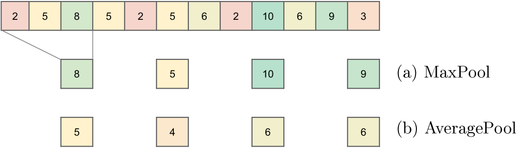
In Section 3 we described the multi-rate signal sampling enhancement of the N-HiTS architecture. Here we conduct a study to compare the accuracy effects of different pooling alternatives, on Equation (1). We consider the MaxPool and AveragePool configurations.

As shown in Table A6, the MaxPool operation consistently outperforms the AveragePool alternative, with MAE improvements up to 15% and MSE up to 8% in the most extended horizon. On average, the forecasting accuracy favors the MaxPool method across the datasets and horizons.

Table A6: Empirical evaluation of long multi-horizon multivariate forecasts for N-HiTS with different pooling configurations. All other hyperparameters were kept constant across all datasets. MAE and MSE for predictions averaged over eight seeds, the best result is highlighted in bold (lower is better). Average percentage difference relative to average pooling in the last panel.

		MaxPool		AveragePool
		MSE	MAE	MSE	MAE
ETTm₂	96	0.185	0.265	0.186	0.262
	192	0.244	0.308	0.257	0.315
	336	0.301	0.347	0.312	0.356
	720	0.429	0.438	0.436	0.447
ECL	96	0.152	0.257	0.181	0.290
	192	0.172	0.275	0.212	0.320
	336	0.197	0.304	0.238	0.343
	720	0.248	0.347	0.309	0.400
Exchange	96	0.109	0.232	0.112	0.238
	192	0.280	0.375	0.265	0.371
	336	0.472	0.504	0.501	0.502
	720	1.241	0.823	1.610	0.942
TrafficL	96	0.405	0.286	0.468	0.332
	192	0.421	0.297	0.490	0.347
	336	0.448	0.318	0.531	0.371
	720	0.527	0.362	0.602	0.400
Weather	96	0.164	0.199	0.167	0.200
	192	0.224	0.255	0.226	0.255
	336	0.285	0.311	0.284	0.297
	720	0.366	0.359	0.360	0.352
P. Diff.	96	-8.911	-6.251	0.000	0.000
	192	-7.544	-6.085	0.000	0.000
	336	-8.740	-4.575	0.000	0.000
	720	-15.22	-8.318	0.000	0.000

Interpolation Configurations

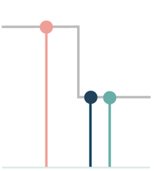
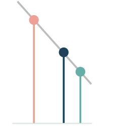
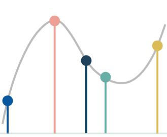
In Section 3 we described the hierarchical interpolation enhancement of the multi-step prediction strategy. Here we conduct a study to compare the accuracy effects of different interpolation alternatives. To do it, we change the interpolation technique used in the multi-step forecasting strategy of the N-HiTS architecture. The interpolation techniques considered are nearest neighbor, linear and cubic. We describe them in detail below.

Recalling the notation from Section 3, consider the time indexes of a multi-step prediction $\tau\in\{t+1,\dots,t+H\}$ , let $\mathcal{T}=\{t+1,t+1+1/r_{\ell}\dots,t+H\}$ be the anchored indexes in N-HiTS layer $\ell$ , and the forecast $\hat{y}_{\tau,\ell}=g(\tau,\boldsymbol{\theta}^{f}_{\ell})$ and backast $\tilde{y}_{\tau,\ell}=g(\tau,\boldsymbol{\theta}^{f}_{\ell})$ components. Here we define different alternatives for the interpolating function $g\in\mathcal{C}^{0},\mathcal{C}^{1},\mathcal{C}^{2}$ . For simplicity we skip the $\ell$ layer index.

Nearest Neighbor. In the simplest interpolation, we use the anchor observations in the time dimension closest to the observation we want to predict. Specifically, the prediction is defined as follows:

\hat{y}_{\tau}=\theta[t^{*}]\quad\text{with}\quad t^{*}=\text{argmin}_{t\in\mathcal{T}}\{|t-\tau|\}

(10)

Linear. An efficient alternative is the linear interpolation method, which uses the two closest neighbor indexes $t_{1}$ and $t_{1}$ , and fits a linear function that passes through both.

\hat{y}_{\tau}=\left(\theta[t_{1}]+\left(\frac{\theta[t_{2}]-\theta[t_{1}]}{t_{2}-t_{1}}\right)(\tau-t_{1})\right)

(11)

Cubic. Finally we consider the Hermite cubic polynomials defined by the interpolation constraints for two anchor observations $\theta_{t_{1}}$ and $\theta_{t_{1}}$ and its first derivatives $\theta^{{}^{\prime}}_{t_{1}}$ and $\theta^{{}^{\prime}}_{t_{1}}$ .

\hat{y}_{\tau}=\theta[t_{1}]\phi_{1}(\tau)+\theta[t_{2}]\phi_{2}(\tau)+\theta^{{}^{\prime}}[t_{1}]\psi_{1}(\tau)+\theta^{{}^{\prime}}[t_{2}]\psi_{2}(\tau)

(12)

With the Hermite cubic basis defined by:


	$\displaystyle\phi_{1}(\tau)=2\tau^{3}-3\tau^{2}+1$		(13a)
	$\displaystyle\phi_{2}(\tau)=-2\tau^{3}+3\tau^{2}$		(13b)
	$\displaystyle\psi_{1}(\tau)=\tau^{3}-2\tau^{2}+\tau$		(13c)
	$\displaystyle\psi_{2}(\tau)=\tau^{3}-\tau^{2}$		(13d)

The ablation study results for the different interpolation techniques are summarized in Table A7, we report the average MAE and MSE performance across the five datasets. Figure 4 presents the decomposition for the different interpolation techniques. We found that linear and cubic interpolation consistently outperform the nearest neighbor alternative, and show monotonic improvements relative to the nearest neighbor technique along the forecasting horizon.

The linear interpolation improvements over nearest neighbors are up to 15.8%, and up to 7.0% for the cubic interpolation. When comparing between linear and cubic the results are inconclusive as different datasets and horizons slight performance differences. On average across the datasets both the forecasting accuracy and computational performance favors the linear method, with which we conducted the main experiments of this work with this technique.

Table A7: Empirical evaluation of long multi-horizon multivariate forecasts for N-HiTS with different interpolation configurations. All other hyperparameters were kept constant across all datasets. MAE and MSE for predictions averaged over eight seeds, the best result is highlighted in bold (lower is better). Percentage difference relative to n. neighbor in the last panel, average across datasets.

		Linear		Cubic		N.Neighbor
		MSE	MAE	MSE	MAE	MSE	MAE
ETTm₂	96	0.185	0.265	0.179	0.256	0.180	0.259
	192	0.244	0.308	0.241	0.303	0.252	0.315
	336	0.301	0.347	0.314	0.358	0.302	0.351
	720	0.429	0.438	0.439	0.450	0.442	0.455
ECL	96	0.152	0.257	0.149	0.252	0.151	0.255
	192	0.172	0.275	0.174	0.279	0.175	0.279
	336	0.197	0.304	0.190	0.295	0.211	0.318
	720	0.248	0.347	0.256	0.353	0.263	0.358
Exchange	96	0.109	0.232	0.1307	0.254	0.126	0.248
	192	0.280	0.375	0.247	0.357	0.357	0.416
	336	0.472	0.504	0.625	0.560	0.646	0.560
	720	1.241	0.823	1.539	0.925	1.740	0.973
TrafficL	96	0.405	0.286	0.402	0.282	0.405	0.359
	192	0.421	0.297	0.417	0.295	0.419	0.201
	336	0.448	0.318	0.446	0.315	0.445	0.253
	720	0.527	0.362	0.540	0.366	0.525	0.318
Weather	96	0.164	0.199	0.162	0.203	0.161	0.360
	192	0.224	0.255	0.225	0.257	0.218	0.928
	336	0.285	0.311	0.285	0.304	0.298	0.988
	720	0.366	0.359	0.380	0.369	0.368	1.047
P. Diff.	96	-0.907	-0.717	0.146	1.61	0.000	0.000
	192	-5.582	-3.259.	-7.985	-4.332	0.000	0.000
	336	-10.516	-4.199	-2.108	-1.455	0.000	0.000
	720	-15.800	-7.042	-5.480	-1.579	0.000	0.000

Order of Hierarchical Representations

Deep Learning in classic tasks like computer vision and natural language processing is known to learn hierarchical representations from raw data that increase complexity as the information flows through the network. This automatic feature extraction phenomenon is believed to drive to a large degree the algorithms’ success (Bengio, Courville, and Vincent 2012). Our approach differs from the conventions in the sense that we use a Top-Down hierarchy where we prioritize in the synthesis of the predictions to low frequencies and sequentially complement them with higher frequencies details, as explained in Section 3. We achieve this with N-HiTS’ expressiveness ratio schedules. Our intuition is that the Top-Down hierarchy acts as a regularizer and helps the model to focus on the broader factors driving the predictions rather than narrowing its focus at the beginning on the details that compose them. To test these intuitions, we designed an experiment where we inverted the expressiveness ratio schedule into Bottom-Up hierarchy predictions and compared the validation performance.

Remarkably, as shown in Table A8, the Top-Down predictions consistently outperform the Bottom-Up counterpart. Relative improvements in MAE are 4.6%, in MSE of 7.5%, across horizons and datasets. Our observations match the forecasting community practice that addresses long-horizon predictions by first modeling the long-term seasonal components and then its residuals.

Table A8: Empirical evaluation of long multi-horizon multivariate forecasts for N-HiTS with different hierarchical orders. All other hyperparameters were kept constant across all datasets. MAE and MSE for predictions averaged over eight seeds, the best result is highlighted in bold (lower is better). Average percentage difference relative to ascending hierarchy in the last panel.

		Top-Down		Bottom-Up
		MSE	MAE	MSE	MAE
ETTm₂	96	0.185	0.265	0.191	0.266
	192	0.244	0.308	0.261	0.320
	336	0.301	0.347	0.302	0.353
	720	0.429	0.438	0.440	0.454
ECL	96	0.152	0.257	0.164	0.270
	192	0.172	0.275	0.186	0.292
	336	0.197	0.304	0.217	0.327
	720	0.248	0.347	0.273	0.369
Exchange	96	0.109	0.232	0.114	0.242
	192	0.280	0.375	0.436	0.452
	336	0.472	0.504	0.654	0.574
	720	1.241	0.823	1.312	0.861
TrafficL	96	0.405	0.286	0.410	0.292
	192	0.421	0.297	0.427	0.305
	336	0.448	0.318	0.456	0.323
	720	0.527	0.362	0.557	0.379
Weather	96	0.164	0.199	0.163	0.200
	192	0.224	0.255	0.219	0.252
	336	0.285	0.311	0.288	0.311
	720	0.366	0.359	0.365	0.355
P. Diff.	96	-2.523	-2.497	0.000	0.000
	192	-12.296	-6.793	0.000	0.000
	336	-11.176	-5.507	0.000	0.000
	720	-4.638	-3.699	0.000	0.000

Appendix H Multi-rate sampling and Hierarchical Interpolation beyond N-HiTS

Empirical observations let us infer that the advantages of the N-HiTS architecture are rooted in its multi-rate hierarchical nature, as both the multi-rate sampling and the hierarchical interpolation complement the long-horizon forecasting task in MLP-based architectures. In this ablation experiment, we quantitatively explore the effects and complementarity of the techniques in an RNN-based architecture.

This experiment follows the Table 2 ablation study, reporting the average performance across ETTm $2$ , ECL, Exchange, TrafficL, and Weather datasets. We define the following set of alternative models: DilRNN₁, our proposed model with both multi-rate sampling and hierarchical interpolation, DilRNN₂ only hierarchical interpolation, DilRNN₃ only multi-rate sampling, DilRNN with no multi-rate sampling or interpolation (corresponds to the original DilRNN (Chang et al. 2017)).

Tab. A9 shows that the hierarchical interpolation technique drives the main improvements (DilRNN₂), while the combination of both proposed components (hierarchical interpolation and multi-rate sampling) sometimes results in the best performance (DilRNN₁), the difference is marginal. Contrary to the clear complementary observed in Table 2, the DilRNN does not improve substantially from the multi-rate sampling techniques. We find an explanation in the behavior of the RNN that summarizes past inputs and the current observation of the series, and not the complete whole past data like the MLP-based architectures.

A key takeaway of this experiment is that N-HiTS’ hierarchical interpolation technique exhibits significant benefits in other architectures. Despite these promising results, we decided not to pursue more complex architectures in our work as we found that the interpretability of the N-HiTS predictions and signal decomposition capabilities was not worth losing.

Table A9: Empirical evaluation of long multi-horizon multivariate forecasts for DilRNN with/without enhancements. Average MAE and MSE for five datasets, the best result is highlighted in bold, second best in blue (lower is better).

		DilRNN₁	DilRNN₂	DilRNN₃	DilRNN
A. MSE	96	0.346	0.331	0.369	0.347
	192	0.539	0.528	0.545	0.561
	336	0.647	0.691	0.705	0.723
	720	0.765	0.762	0.789	0.800
A. MAE	96	0.343	0.335	0.352	0.347
	192	0.460	0.444	0.462	0.468
	336	0.513	0.537	0.539	0.649
	720	0.585	0.566	0.600	0.598

Appendix I Hyperparameter Optimization Resources

Computational efficiency has implications for the prediction’s accuracy and the cost of deployment. Since forecasting systems are constantly retrained to address distributional shifts, orders-of-magnitude improvements in speed can easily translate into orders-of-magnitude price differences deploying the models. This section explores the implications of computational efficiency in the accuracy gains associated with hyperparameter optimization and training economic costs.

Hyperparameter Optimization. Despite all the progress improving the computation efficiency of Transformer-based methods, see Figure 4, their speed and memory requirements make exploring their hyperparameter space unaffordable in practice, considering the amount of GPU computation they still require.

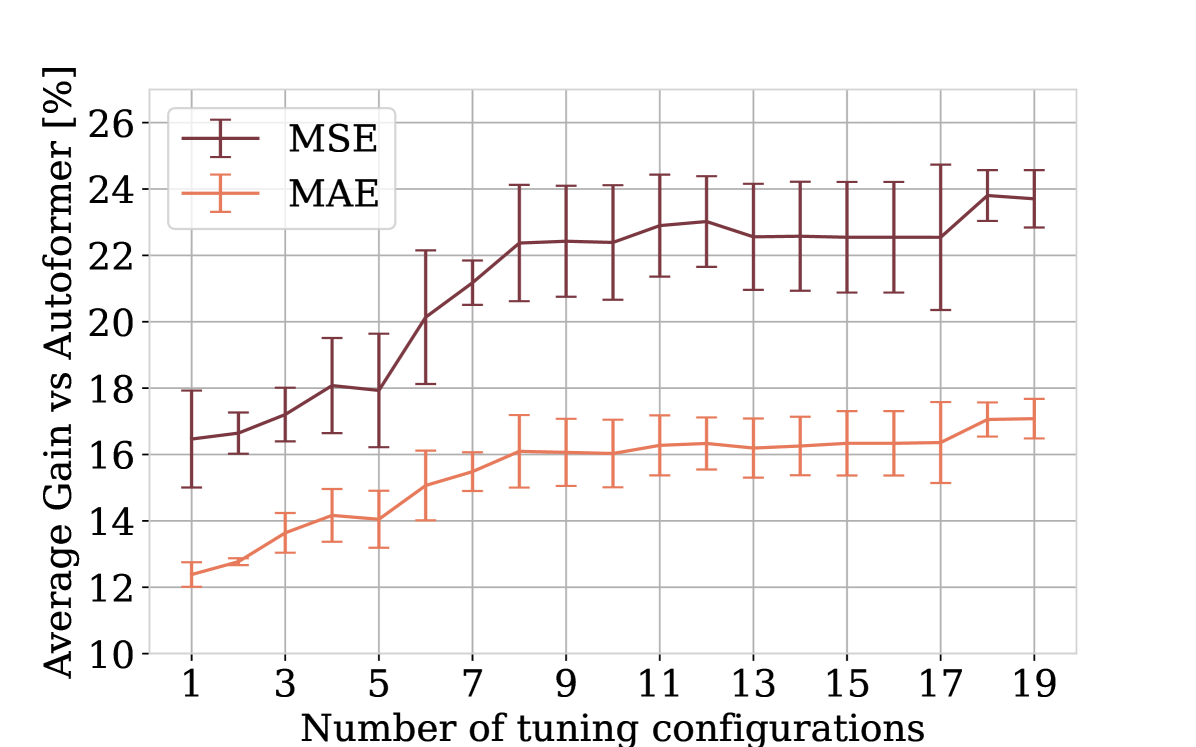
For this experiment we report the iterations of the hyperparameter optimization phase, described in Section 4, where we explore the hyperparameters from Table A3 using HYPEROPT, a Bayesian hyperparameter optimization library (Bergstra et al. 2011). As shown in Figure 6 the exploration exhibits monotonic relative performance gains of N-HiTS versus the best reported Autoformer (Wu et al. 2021) in the ablation datasets.

Training Economic Costs. We measure the train time for N-HiTS, N-BEATSg and Transformer-based models, on the six main experiment datasets and 8 runs. We rely on a AWS g4dn.2xlarge, with an NVIDIA T4 16GB GPU.

We differentiate between N-HiTS₁, our method with a single HYPEROPT iteration randomly sampled from Table A3, and N-HiTS₂₀ to our method after 20 HYPEROPT iterations. For the Transformer-based models we used optimal hyperparameters as reported in their repositories. Table A10 shows the measured train time for the models, N-HiTS₁ takes 1.5 hours while more expensive architectures like Autoformer or Informer take 92.6 and 62.1 hours each. Based on hourly prices from January 2022 for the g4dn.2xlarge instance, USD 0.75, the main results of the paper would cost nearly USD 70.0 with Autoformer, USD 46.5 with Informer, while N-HiTS₁ results can be executed under USD 1.5 and N-HiTS₂₀ with USD 22.8. Figure 6, shows that N-HiTS₁ achieves a 17% MSE average performance gain over Autoformer with 1.6% of a single run cost, and N-HiTS₂₀ almost 25% gain with 33% of a single run cost. A single run does not consider hyperparameter optimization.

\text{ExptPrice}=\text{GPUPrice}\times\text{HyperOptIters}\times\text{TrainTime}\times\text{Runs}

Table A10: Train time in hours on a g4dn.2xlarge instance.

	Horizon	N-HiTS₁	N-HiTS₂₀	Autoformer	Informer	N-BEATSg
A. Time	96/24	0.183	3.66	12.156	9.11	0.291
	192/36	0.257	5.14	16.734	11.598	0.462
	336/48	0.398	7.96	22.73	15.237	0.674
	720/60	0.682	13.64	40.987	26.173	1.249
	Total	1.523	30.46	92.607	62.118	2.676