Narrowing the gaps of the missing Blaschke-Santaló diagrams
Abstract.
We solve several new sharp inequalities relating three quantities amongst the area, perimeter, inradius, circumradius, diameter, and minimal width of planar convex bodies. As a consequence, we narrow the missing gaps in each of the missing planar Blaschke-Santaló diagrams. Furthermore, we extend some of those sharp inequalities into higher dimensions, by replacing either the perimeter by the mean width or the area by the volume.
September 6, 2025
1. Introduction
In 1916 Blaschke [3] raised the question of determining the set of triples given by the volume , surface area , and integral mean curvature of every set from the set of -dimensional convex bodies . To do so, he defined the function
and studied the set of images of , which is known as the Blaschke diagram. Despite recent efforts (see [29] or [33]) this diagram still today remains unsolved.
Years later, Santaló [34] proposed the study of possible triples for the geometric quantities area , perimeter , inradius , circumradius , diameter , and minimum width of a -dimensional convex body. As a result, he already solved the cases , , , , , and . Later on Hernández Cifre and Segura Gomis in [19] and [23] concluded the quest to describe the diagrams , , , Hernández Cifre completely described in [20] the diagrams and , Böröczky Jr., Hernández Cifre, and Salinas described the diagrams and in [5], and very recently Delyon, Henrot, and Privat completely described in [12] the diagram .
Those functionals have been also considered in other diagrams. For instance, it has been described the case in [6] as well as an almost complete description by Ting and Keller of in [38]. Furthermore, Hernández Cifre et al. described in [21] diagrams for the inradius, circumradius, and volume and surface area for -dimensional centrally symmetric convex bodies. In [7] the authors described detailed diagrams when the functionals are measured with respect to other balls different from the Euclidean ball, such as the triangle, square, pentagon, or hexagon, or a general convex body. Very recently in [10] the authors studied diagrams for other notions of diameters.
More diagrams have been recently studied when introducing other functionals. Ftouhi and Lamboley [16] have described the diagram for the area, perimeter, and the first Dirichlet eigenvalue, Lucardesi and Zucco [28] described the diagram for the area, the torsional ridigity, and the first Dirichlet eigenvalue (see also Buttazzo and Pratelli [11] for more information on this diagram), Ftouhi and Henrot [15] studied the diagram for the area, the first Dirichtel eigenvalue, and the first non-trivial Laplacian-Neumann eigenvalue, and also Ftouhi [14] computed the diagram of the area, perimeter, and the Cheeger constant. Very recently Gastaldello, Henrot, and Lucardesi in [17] have studied the diagram of area, perimeter, and moment of inertia.
The aim of this paper is to solve several new inequalities relating three of the six functionals proposed by Santaló, and to clarify what is known up to date in the matter. This is why we state and prove each new result in the corresponding section. Indeed, we devote a section to each of the six unsolved diagrams, with the exception of and which use a common one.
2. Previous inequalities
Let be the set of -dimensional convex bodies, i.e., convex and compact sets in different from points.
For every , , , let be the scalar product of and . Moreover, let be the Euclidean norm of . Furthermore, let be the vectors of the canonical base of .
Let . The circumradius (resp. inradius) (resp. ) of is the smallest (resp. largest) radius of an Euclidean ball containing (resp. contained in ). The diameter of is the largest Euclidean length between two points contained in . The (minimum) width is the minimum distance between two parallel hyperplanes containing between them. For every , let be the perimeter of . For every , let be its volume or Lebesgue measure, and if , realize that coincides with the usual area .
These functionals are monotonically increasing with respect to inclusion, i.e., if , then for and if then for too. Moreover, if then is -homogeneous, i.e. and . In the case of the volume, it is -homogenous, i.e. , for every and , and thus is -homogeneous.
Some remarkable examples of planar convex bodies are the Euclidean unit ball , the equilateral triangle of unit circumradius , the line segment of edge length , and the Reuleaux triangle of unit circumradius . A body is of constant width if (see [30] for further details). In -dimensional space , let be the -dimensional Euclidean unit ball, thus having that .
Since this is eminently a paper devoted to planar sets, when we refer to some result, we will directly specify its -dimensional version. Moreover, for the references to most of the known inequalities we will refer to [1] as well as the references therein. However, we state here the inequalities that we need further on.
Pál’s inequality (see [32]) provides a lower bound of in terms of , namely
| (2) |
with equality if and only if . If is moreover assumed to be of constant width, then the inequality strengthens onto
| (3) |
known as the Blaschke-Lebesgue inequality (see [4] or [27]), with equality if and only if .
Further trivial inequalities between the area and the circumradius and inradius are
with equality if and only if .
The perimeter and the diameter relate as
| (4) |
where the left inequality is trivial and gets equal when , and the right one is a consequence of Barbier [2] and it becomes equality when is a constant width set.
The perimeter and the inradius fulfill the trivial inequality with equality for . The perimeter and the circumradius fulfill
| (5) |
where the left inequality attains equality when , and the right inequality gets equal when .
The relation between the perimeter and the width is described by
| (6) |
as a consequence of Cauchy’s formula (see [35]), with equality if and only if is of constant width.
In [5] it was proven the optimal lower bound for the perimeter in terms of the inradius and the circumradius, namely:
| (7) |
Moreover, equality holds if and only if is the convex hull of a point, its mirrored with the origin, and an euclidean ball centered at the origin.
In [25] the author derived the optimal upper bound of the perimeter in terms of the diameter and the width
| (8) |
Moreover, equality holds for the intersection of the Euclidean ball centered at the origin with a halfspace and its mirrored with respect to the origin.
The quotient between the circumradius and the diameter is described by Jung’s inequality [24]
| (9) |
with equality if and only if contains an equilateral triangle of circumradius and diameter .
The relation between the inradius and the width is described by
| (10) |
where the left side attains equality if and only if and the right side, known as Steinhagen’s inequality [37], becomes equality if and only if .
The relation between the circumradius and the width is described by
with equality if and only if .
Finally, if is of constant width, it is known that with equality if and only if . This last statement is a consequence of (9) and the fact that constant width sets attain equality in the concentricity inequalities
| (11) |
(see [8] for more information on these inequalities). Moreover, precisely in the case of constant width sets, one can obtain the sharpened Steinhagen’s inequality
| (12) |
with equality if and only if .
Let . Given a hyperplane , we say that is the Steiner symmetrization of with respect to if for every , is a segment centered around , and it has the same length than . It is well known that , , , , and if then and (see [35]).
For every , let , , and be the affine, linear, and convex hull of , respectively. Given , we let be the line segment with endpoints and . Let to be the boundary of .
The circumball is characterized by some touching conditions of boundary points (see for instance [9]).
Proposition 2.1.
Let with . The following are equivalent:
-
(1)
.
-
(2)
There exist , , , fulfilling the property that .
An analogous result applies to the inradius, namely, if , then if and only if there exist , , , such that . In particular, the points coincide with outer normals of and , and thus, whenever and , the intersection of the halfspaces determined by the orthogonal lines to each containing , , determines a triangle with the property that
| (13) |
3. (A,p,D)
We expose the best known inequalities relating the three quantities , , and for .
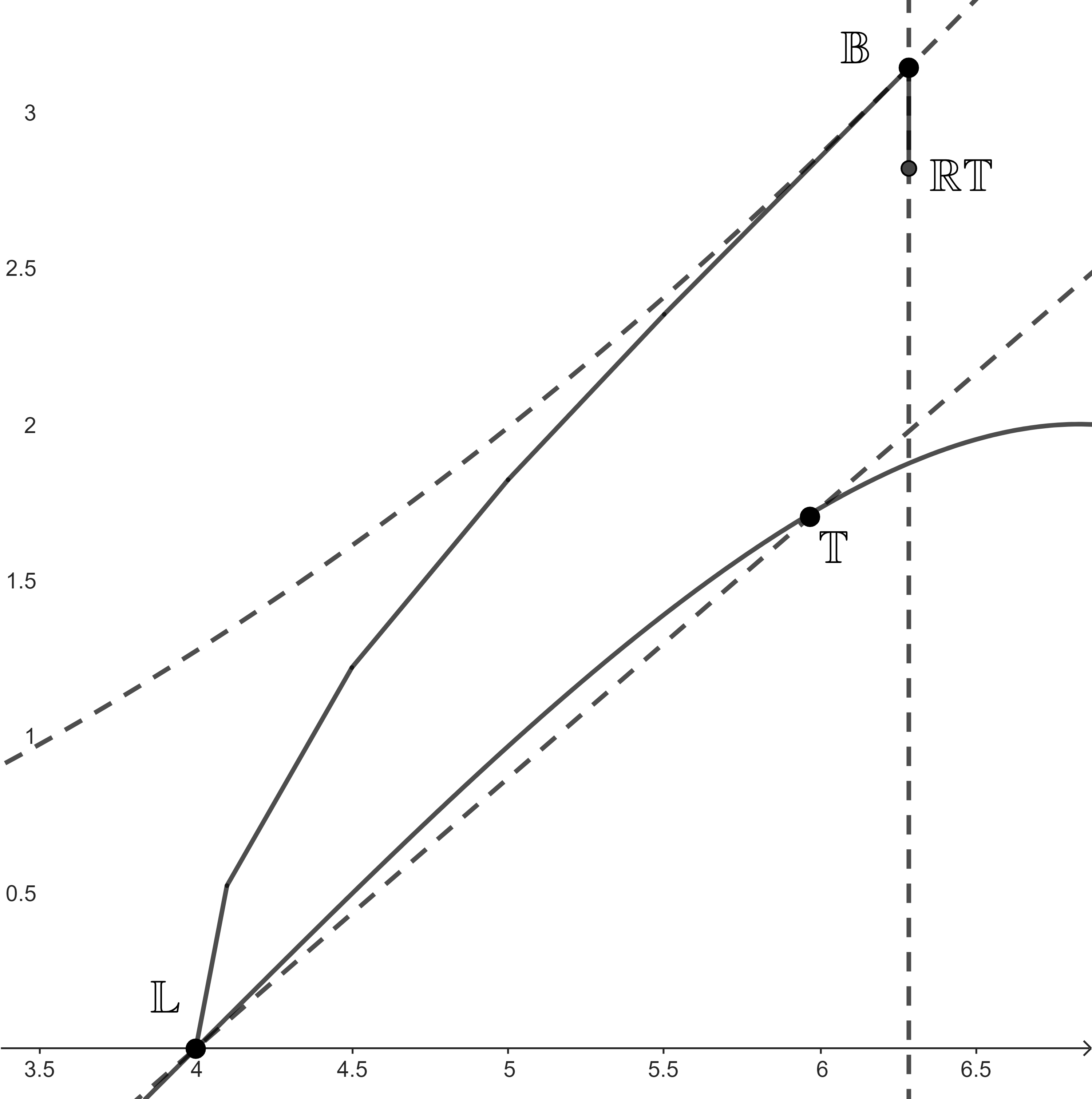
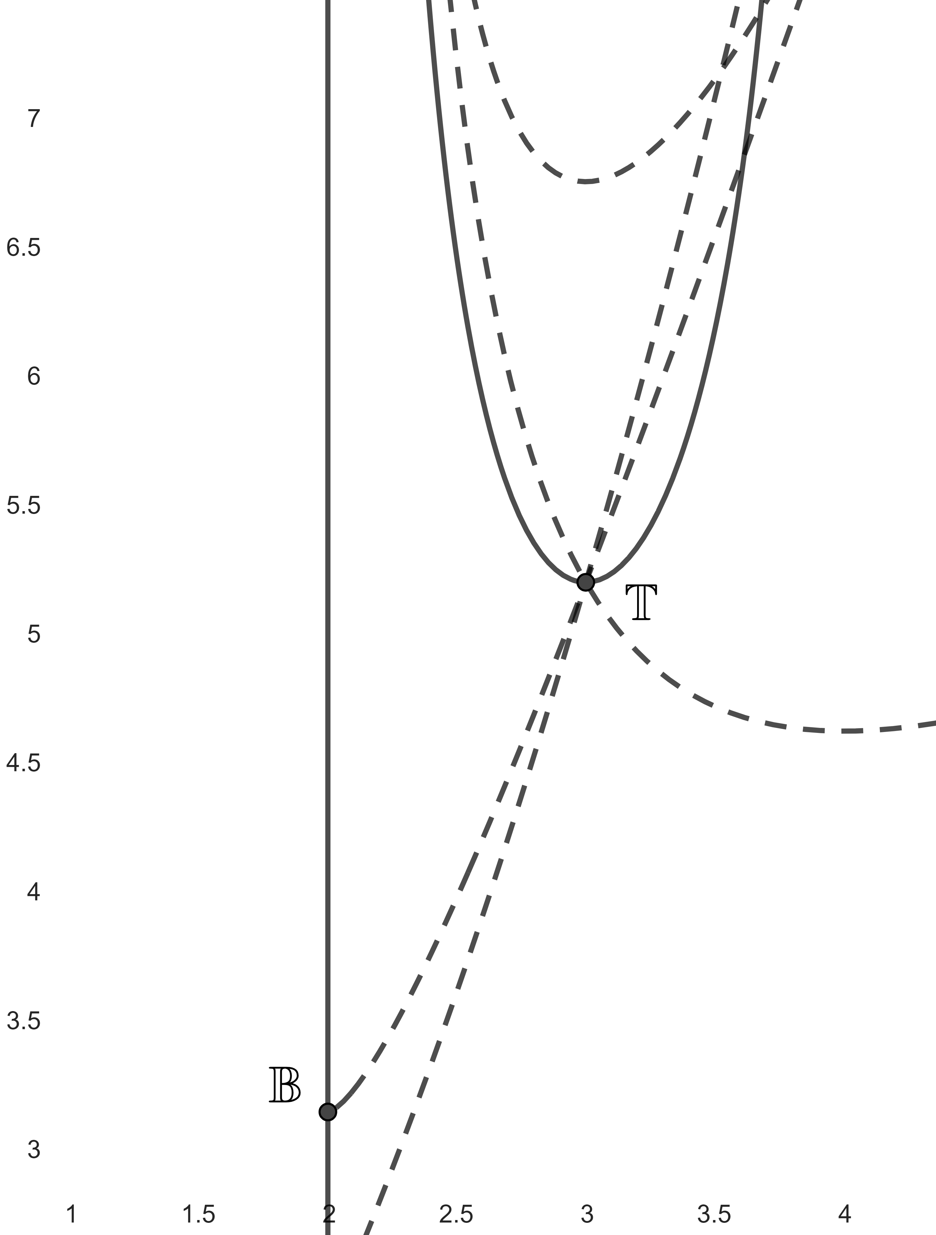
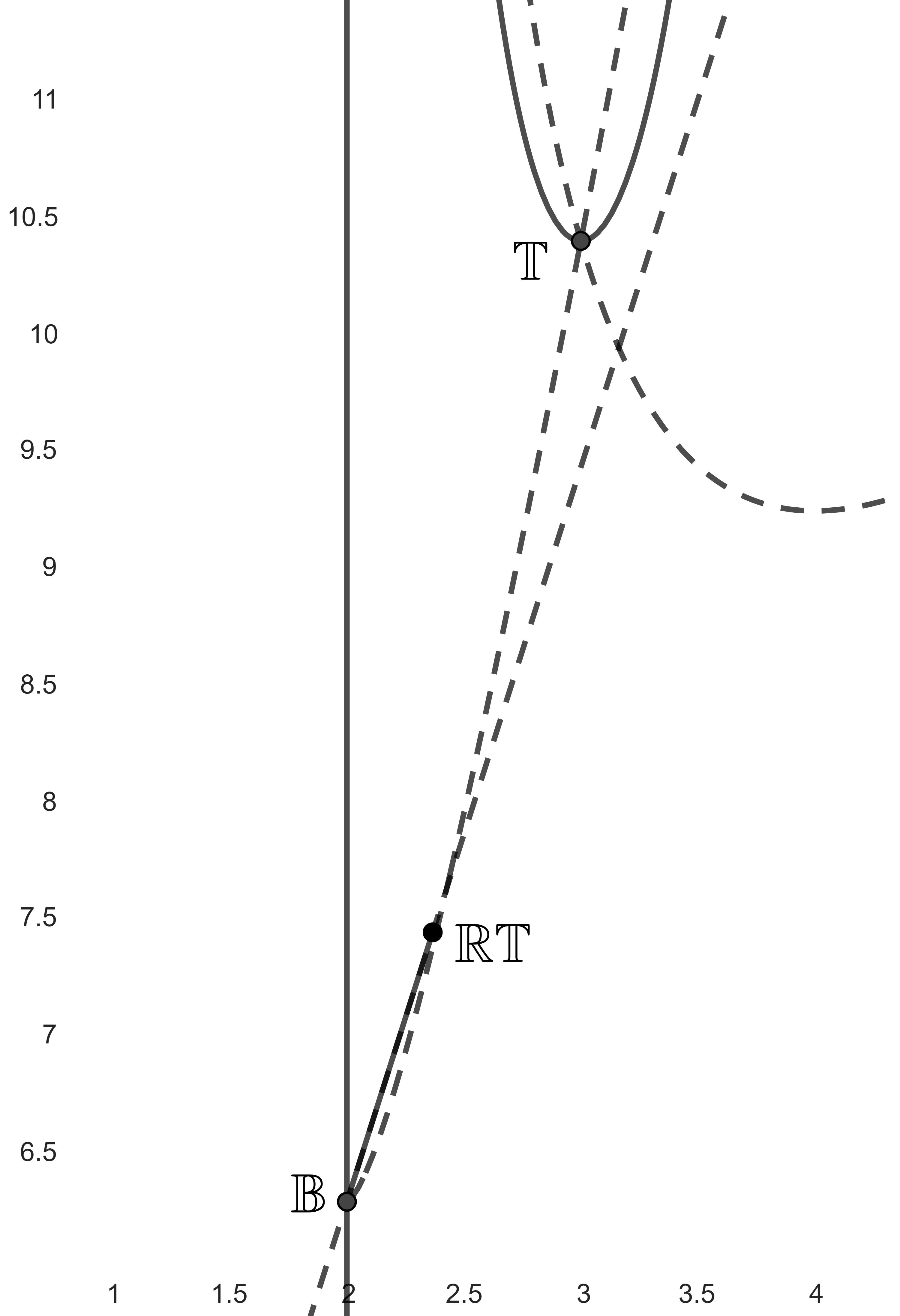
First of all, notice that (4) induces a linear boundary of the diagram . Indeed, fulfills (4) with equality if and only if is of constant width. In particular, from (1) and (3) we know that if is of constant width with , then , with and attaining the lowest and highest values (see Figure 1).
Second, Kubota [25] proved that
| (14) |
where is defined to be solution of , with equality for being a symmetric lenses, i.e., the intersection of two Euclidean balls of the same diameter. It is worth mentioning that (14) implies a strengthening of the isoperimetric inequality (1) (see Figure 1111Here and on each other diagram, we represent valid inequalities by lines. In case of continuous lines, we refer to real boundaries of the diagram; in case of dashed lines, not. If we draw on a diagram, it coincides with the value of its image through the corresponding diagram.).
Third, Kubota [25, 26] also proved that if then
| (15) |
with equality for isosceles triangles with two equal longer edges, having as extreme cases and . Moreover, in the case of , he also proved the inequality
| (16) |
with equality only when .
4. (p,D,r)
It is also known that the right-hand side of (4) induces part of the upper boundary of the diagram, where constant width sets attain equality, and with extreme points at (due to (12)) and .
We now establish a new inequality, providing the lower boundary of this diagram.
Theorem 4.1.
Proof.
After a translation and rescaling of , let us assume that with . Moreover, let , for some .
Notice that . Indeed, assume that (as otherwise and the result is true). since , if we would have that , then by the convexity of we can easily find an Euclidean ball of strictly larger radius than within , thus contradicting the definition of .
By convexity, we have that , and thus by monotonicity of then . Notice that and .
Moreover, since , then , and thus the lines support . Let be the Steiner symmetrization of with respect to the line . It is clear that
where . Since , then . Moreover, it is also clear that every vertical line intersecting is a line segment of length at most , and so . This, together with implies that . By properties of the Steiner symmetrization we know that .
Now again, we do another Steiner symmetrization of , this time with respect to the line . We still have all previous properties inherited from on . It is easy and almost analogous to check that , , and that . Finally, letting , we can clearly see that
Let us now compute , for given values and . To do so, let us compute the only line with negative slope supporting and passing through . Let , , be this line, such that it is tangent to , i.e. such that
has a unique solution. Substituting onto the second equations gives , i.e. . This equation has a unique solution - root - if and only if , i.e. if and only if . In this case, the intersecting point between the line and the circumpherence has coordinates
Since is symmetric with respect to , , its perimeter equals four times its perimeter on the first orthant. Since the angle of with the horizontal line equals , we can conclude that
In order to derive (18), we simply apply the above inequality to (which has diameter ) and use the -homogeneity of and .
Moreover, it is clear from the construction that every set , for every , attains equality in (18). ∎
We now derive an easy non tight upper bound of the diagram as a consequence of (8).
Corollary 4.2.
Let . Then
| (19) |
5. (p,R,w)
The inequality (6) induces part of the right boundary of the diagram. Remember that belongs to this boundary if and only if is of constant width. One of the extreme points is . On the other hand, if is of constant width, i.e. , together with (9), implies that , with equality when . Thus, this last set is the other extreme point of this boundary.
We now show a new inequality which induces the upper boundary of the diagram.
Theorem 5.1.
Proof.
After a suitable dilatation and rigid motion, we can assume that with , and such that the lines and support , where with , i.e.
Above, we take the lines containing between them. This is due to Proposition 2.1, since a consequence of with is that . In particular , and thus . If we denote by the arc of in the region , the arc of in the region , , the line-segment of within , and the line-segment of within , then it is clear that
Notice that
We aim to show that the above expression is nonnegative whenever (which would imply that is nondecreasing on ). To do so, notice that it would then be enough to show that the function is decreasing for every . Since
for every , the assertion holds. Therefore
In order to conclude the proof of the inequality, we simply replace by and use the homogeneity of the functionals and .
Evidently, equality holds for every , for every . ∎
Corollary 5.2.
Let . Then
| (21) |
Moreover, equality holds if .
Proof.
Let us suppose that , , and . Notice that is an increasing function in since . Hence, using (10) in combination with (7) we get that
We then obtain the desired result when applying the above inequality to the set and using the -homogeneity of and .
Evidently, when we attain equality in (21). ∎
6. (A,R,w)
Apparently, the only two known inequalities relating this triple are
| (22) |
(see [18]) with both inequalities having equality if , and the left-hand side also attaining equality at .
The first inequality we prove induces the upper boundary of the diagram.
Theorem 6.1.
Proof.
After a translation and dilatation, let us assume that with . Moreover, after a suitable rotation, let us assume that the lines supporting with width are given by the equations and , for some such that , i.e.
Above, we take the lines containing between them. This is due to Proposition 2.1, since a consequence of with is that . In particular, we have that
Thus . Notice that and . Now let us compute . Notice that is the union of four triangles and two circular sectors as in Figure 5.
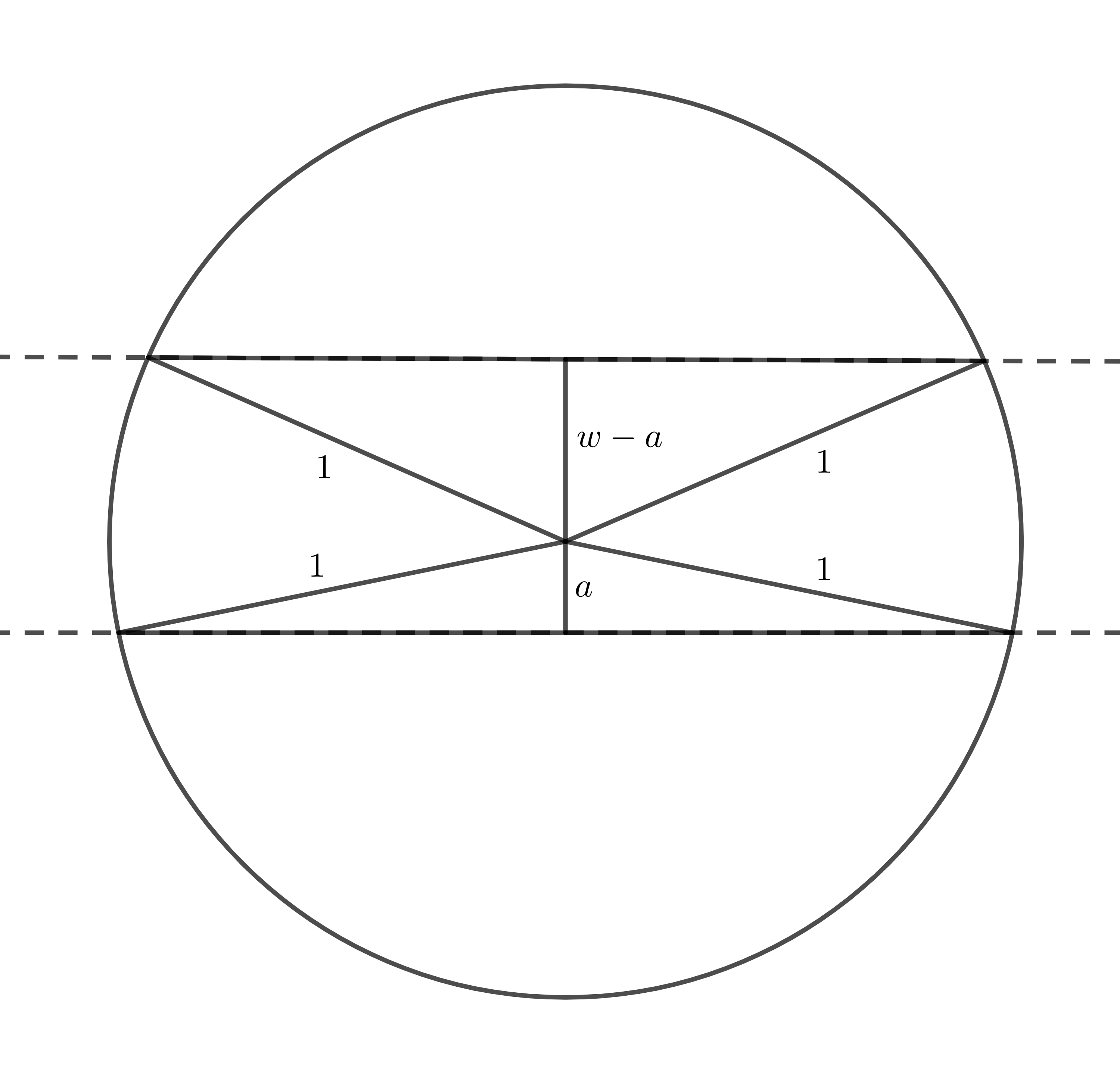
The areas of the triangles are and (twice each). The area of each of the circular sectors is . Thus
Notice that
We aim to show that whenever . This is equivalent to show
for , i.e., that is a decreasing function. Since this last statement is true, we conclude that , from which
In order to retrieve (23), we only need to replace above by and use the -homogeneity of as well as the -homogeneity of .
Evidently, every body of the form attain equality in (23), for every . ∎
The second inequality we show relating the area, circumradius, and width is one that gives part of the right bound, partly improving (22) for a certain range of values near .
Theorem 6.2.
Let . Then
| (24) |
Moreover, equality holds if .
Proof.
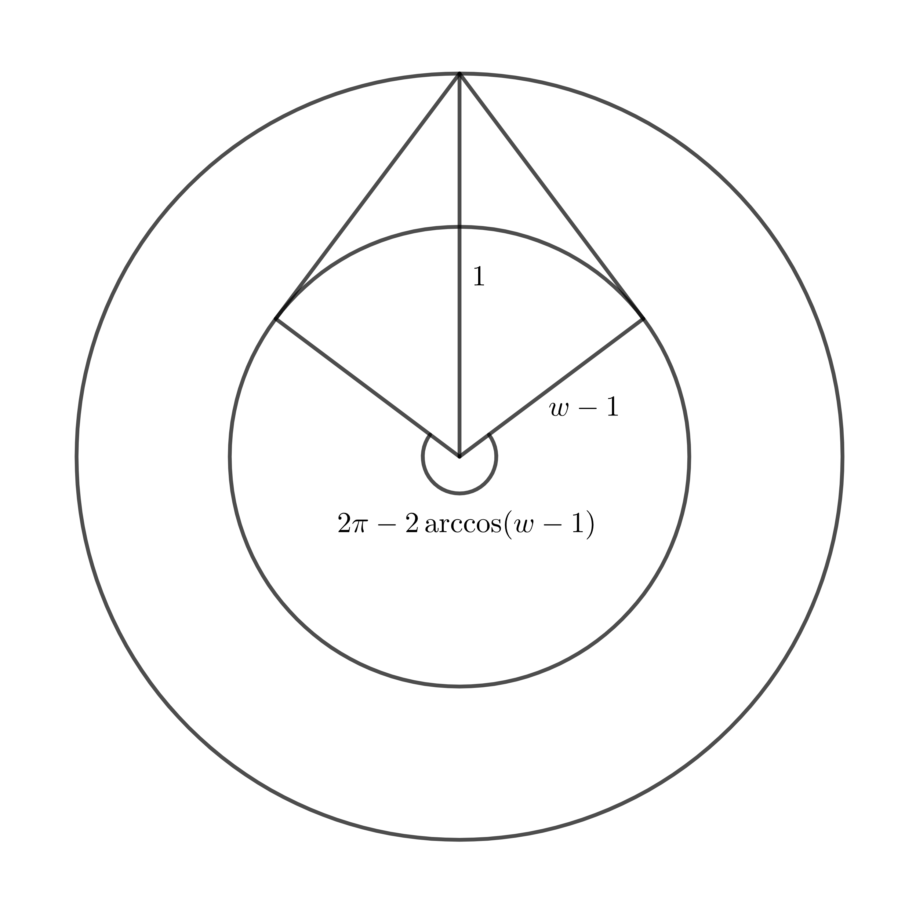
Let us suppose that , , and . Using the fact that (see the left-hand side of (11)), then . Let for some . Moreover, by Proposition 2.1 let , , be such that . Hence , for some , and thus from which at least one of them, say , fulfills . Using the convexity of we get that and thus . Notice that the distance from to is at least , which occurs when . Thus . It is clear that decomposes in a circular sector of angle and radius and two triangles each of area (see Figure 6), and thus
In order to obtain the result, we simply apply the above inequality to the set and take into account the -homogeneity of as well as the -homogeneity of .
Moreover, if we replace by , it is very simple to notice that the inequality above becomes equality.
∎
7. (A,r,w) and (p,r,w)
In this last section we consider both remaining diagrams since the techniques to induce both inequalities are completely analogous.
7.1.
The left-hand side inequality of (10) induces the left unbounded boundary of the diagram, with extreme point at . The best known classic upper bounds so far were the inequalities
| (25) |
(see [36]), where the second one attains equality when . The best lower bound was so far the inequality (2), with equality if and only if (see Figure 7).
7.2.
The left-hand side inequality of (10) induces the left unbounded boundary of the diagram, with extreme point at . Moreover, the inequality (6) provides part of the lower bound of the diagram, with extreme points at and (due to (12)). The best known classic upper bound so far was the inequality
| (26) |
(see [36]), with equality if and only if .
The first result we show is a pair of inequalities which induce the upper boundaries of their respective diagrams.
Theorem 7.1.
Proof.
Let be a triangle such that with (see (13)). Of course we also have that , , and and hence
Let us assume now that , with , and thus the width of is attained in the direction .
In the next step, we will show that replacing the vertex of , , not belonging to by such that the new triangle is an isosceles triangle with , has the properties , , and . To do so, let us consider the points , , and let
Since
we will show that for every , thus showing in particular that . Evidently, whenever ; thus it only remains to show it when . In that case, it is equivalent to show that
which holds if and only if , which is equivalent to the valid inequality .
Thus, replacing by the isosceles would give us (see above), and by Fubini’s theorem that . Hence, using the inradius, perimeter, and area formula of triangles implies that . Evidently, we also have that . Thus
Wrapping up all the above, we have proven that for every there exists an isosceles triangle with two longer edges with
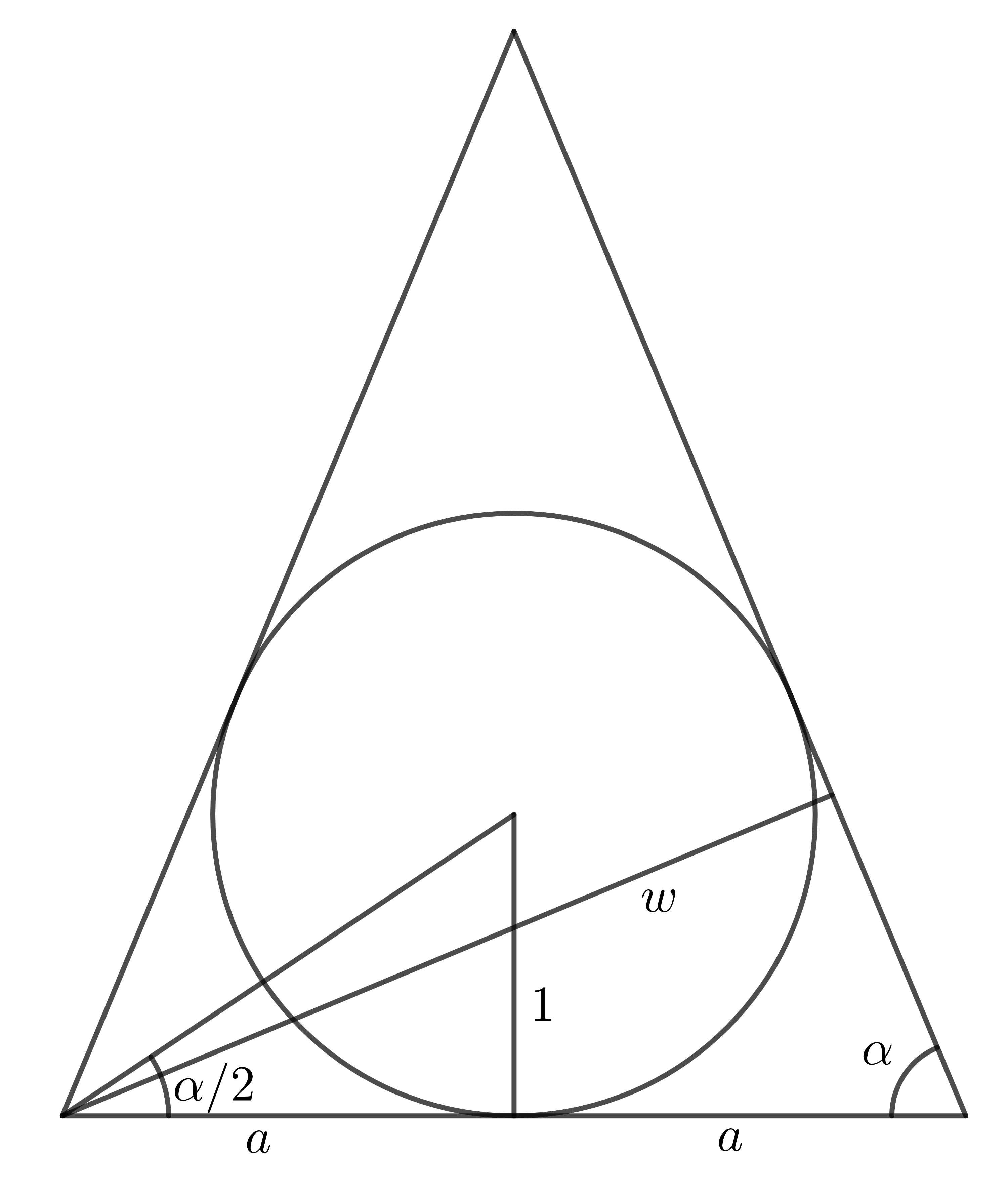
Finally, let be one of the two equal angles of , and let be half of the length of the shorter edge of (see Figure 9). Moreover, let us call , , , and . Using standard trigonometric arguments we obtain that
From there we easily obtain that
(notice that by Steinhagen’s theorem (10)). The base of has length and the corresponding height equals to .
On the one hand, we have that
Since for every , thus is non-increasing. Hence, assuming that too, we conclude that
The inequality is then retrieved by applying the inequality above to and using the -homogeneity of as well as the -homogeneity of .
On the other hand
Since
thus for every , hence getting that is decreasing on . Therefore
In order to obtain the second result, we simply apply the inequality above to and use the -homogeneity of the functionals and .
Moreover, equality holds on each of the inequalities above for every isosceles triangle with two longer equal edges. ∎
We end this section by providing new inequalities that bound from below each of their diagrams. Note that (29) already provides a strenghening of Pál’s inequality (2), whereas (30) improves (6) within a range of values near .
Theorem 7.2.
Let . Then
| (29) |
and
| (30) |
Moreover, equality holds in both inequalities when or .
Proof.
Let be a triangle with such that (see (13)). Let us suppose after a translation and dilatation that with . Let be the edges of , . Since , there exists at distance from , . Notice also that each belongs to one of the three disconnected regions of . Using the convexity of , in particular we would have that
with , for every . Thus and .
We first compute . We have that
Evidently, since the distance from to is at least , we can replace by such that the distance from to is exactly equal to . We now compute . To do so, notice that the region can be seen as a rectangular triangle of hipotenuse and leg equal to of common angle minus the corresponding ball sector from of angle . On the one hand, the area of the triangle equals , and on the other hand the area of the ball sector equals , where . Adding it all, we would conclude that
8. Higher dimensions
Some of the inequalities above can be naturally extended to higher dimensions with not much additional effort. To this aim, let . Moreover, let be the mean width of , i.e. , where is the directional width of in the direction and is the unitary measure over . Let be the surface area measure of . Remember that , where stands for the Gamma function, and that for every . We will stress the subindex in the volume when applied to some in case it helps in avoiding confusion.
If is an -dimensional lineal subspace of , let be the orthogonal projection onto . Moreover, if is -dimensional, then let be the perimeter of measured within . Notice that for every we have that
| (31) |
The first result is an extension of (18) when replacing by .
Theorem 8.1.
Let . Then
| (32) |
Moreover, for every , there exists with , , and such that fulfills (32) with equality.
Proof.
After a translation and rescaling of , let us assume that with . Moreover, let , for some .
It is straighforward to check that (as in the proof of (18)). By convexity, we have that , and thus by monotonicity of then . Notice that and . If we now proceed as in the proof of (18) by applying successive Steiner symmetrizations with respect to the hyperplanes , we would easily conclude that , where , with and .
The inequality (32) is then retrieved by applying the above inequality to the set and using the -homogeneity of the functionals and .
Evidently, equality holds whenever , for every . ∎
The next result is an extension of (20) to higher dimensions, replacing by .
Theorem 8.2.
Let . Then
Moreover, for every , there exists such that , , and fulfills with equality the inequality above.
Proof.
After a suitable dilatation and rigid motion, we can assume that with , and such that the hyperplanes and support , where with , i.e.
In particular , and thus . Evidently, and .
Using (31) and (20) within for every we obtain that
where and , for every . In order to obtain the inequality, one simply needs to replace above by and use the -homogeneity of the functionals and .
Evidently, equality holds whenever , for every . ∎
Let us remember a particular instance of the Eulerian hypergeometric function
for every and (see [13]).
The following result is an extension of (23) to higher dimensions when replacing by .
Theorem 8.3.
Proof.
After a suitable dilatation and rigid motion, we can assume that with , and such that the hyperplanes and support , where with , i.e.
Above, we take the lines containing between them. This is due to Proposition 2.1, since a consequence of with is that . In particular , and thus .
Notice that by Fubini’s principle
Since
it is very easy to show that under the conditions the function is nonnegative. Thus
In order to obtain (33), we simply apply the inequality above to the set and use the -homogeneity of and the -homogeneity of .
Evidently, equality holds for every , for every . ∎
The right-hand side expression on Theorem 8.3 can be explicitly computed avoiding the use of the hypergeometric function.
Remark 8.4.
If for every we denote by
it is well-known that can be computed recursively in terms of when integrating by parts. One can derive that
for absolute constants , , and so on. In particular, Theorem 8.3 is equivalent to (23) when ; if we would then have that
or if , we would obtain that
As mentioned in Theorem (33), sets of the form would attain equality above for every and .
References
- [1] P. W. Awyong, P. R. Scott, Inequalities for convex sets, J. Ineq. Pure Appl. Math. 1 (2000), no. 1, 6.
- [2] E. Barbier, Note sur le problème de l’aiguille et le jeu du joint couvert, J. Math. Pures Appl. 5 (1860), 273–286.
- [3] W. Blaschke, Eine Frage über konvexe Körper, Jahresber, Dtsch. Math.-Ver. 25 (1916), 121–125.
- [4] W. Blaschke, Konvexe Bereiche gegebener konstanter Breite und kleinsten Inhalts, Math. Ann. 76 (1915), no. 4, 504–513.
- [5] K. Böröczky Jr., M. A. Hernández Cifre and G. Salinas, Optimizing area and perimeter of convex sets for fixed circumradius and inradius, Monatsh. Math. 138 (2003), 95–110.
- [6] R. Brandenberg, B. González Merino, A complete 3-dimensional Blaschke-Santaló-diagram, Math. Inequal. Appl. 20 (2017), no. 2, 301–348.
- [7] R. Brandenberg, B. González Merino, Behaviour of inradius, circumradius, and diameter in generalized Minkowski spaces, RACSG 116 (2022), no. 3, 105.
- [8] R. Brandenberg, B. González Merino, Minkowski concentricity and complete simplices, J. Math. Anal. Appl. 454 (2017), no. 2, 981–994.
- [9] R. Brandenberg, S. König, No dimension-independent core-sets for containment under homothetics, Discrete Comput. Geom. 49 (2013), no. 1, 3–21.
- [10] R. Brandenberg, M. Runge, Jung-type inequalities and Blaschke-Santaló diagrams for different diameter variants, in preparation.
- [11] G. Buttazzo, A. Pratelli, An application of the continuous Steiner symmetrization to Blaschke-Santaló diagrams, ESAIM: Control, Optimisation and Calculus of Variations, 27, 36.
- [12] A. Delyon, A. Henrot, and Y. Privat, The missing (A,D,r) diagram, Ann. de l’Institut Fourier. 72 (2022), no. 5.
- [13] A. Erdélyi, W. Magnus, F. Oberhettinger, F. G. Tricomi, Higher transcendental functions, Vol. I. New York – Toronto – London: McGraw–Hill Book Company, Inc, 1953.
- [14] I. Ftouhi, Complete systems of inequalities relating the perimeter, the area and the Cheeger constant of planar domains, Commun. Contemp. Math. page 2250054.
- [15] I. Ftouhi, A. Henrot, The diagram , preprint, hal-03311538v1, 2021.
- [16] I. Ftouhi, J. Lamboley, Blaschke-Santaló diagram for volume, perimeter, and first Dirichlet eigenvalue, SIAM J. Math. Anal. 53 (2021), no. 2, 1670–1710.
- [17] R. Gastaldello, A. Henrot, I. Lucardesi, About the Blaschke-Santaló diagram of area, perimeter and moment of inertia, arXiv:2307.11658.
- [18] M. Henk, G. A. Tsintsifas, Some inequalities for planar convex figures, Elem. Math. 49 (1994), no. 3, 120–125.
- [19] M. A. Hernández Cifre, Is there a planar convex set with given width, diameter and inradius?, Amer. Math. Monthly 107 (2000), 893–900.HC2
- [20] M. A. Hernández Cifre, Optimizing the perimeter and the area of convex sets with fixed diameter and circumradius, Arch. Math. 79 (2002), 147–157.
- [21] M. A. Hernández Cifre, J. A. Pastor, G. Salinas Martínez, S. Segura Gomis, Complete systems of inequalities for centrally symmetric convex sets in the n-dimensional space, Arch. Inequal. Appl. 1 (2003), no. 2, 155–167.
- [22] M. A. Hernández Cifre, G. Salinas, S. Segura Gomis, Complete systems of inequalities, J. Ineq. Pure Appl. Math. 2 (2001), no. 1-10, 1–12.
- [23] M. A. Hernández Cifre, S. Segura Gomis, The missing boundaries of the Santaló diagrams for the cases and , Discr. Comp. Geom. 23 (2000), 381–388.
- [24] H. Jung, Über die kleinste Kugel, die eine räumliche Figur einschliet, J. Reine Angew. Math. 123 (1901), 241–257.
- [25] T. Kubota, Einige Ungleischheitsbezichungen über Eilinien und Eiflächen, Sci. Rep. of the Thoku Univ. Ser. (1), 12 (1923), 45–65.
- [26] T. Kubota, Eine Ungleischheit für Eilinien, Math. Z. 20 (1924), 264–-266.
- [27] H. Lebesgue, Sur le problème des isopérimètres et sur les domaines de largeur constante, Bulletin de la Société Mathématique de France, 7: 72–76.
- [28] I. Lucardesi, D. Zucco, On Blaschke–Santaló diagrams for the torsional rigidity and the first Dirichlet eigenvalue, Ann. di Mat. Pura ed Appl. (1923-) 201 (2022), no. 1, 175–201.
- [29] Y. Martínez-Maure, De nouvelles inégalités géométriques pour les hérissons, Arch. Math. 72 (1999), 444–453.
- [30] H. Martini, L. Montejano, D. Oliveros, Bodies of constant width, Springer International Publishing, 2019.
- [31] R. Osserman, The isoperimetric inequality, Bull. Amer. Math. Soc. 84 (1978), no. 6, 1182–1238.
- [32] J. Pál, Ein Minimal problem für Ovale, Math. Ann. 83 (1921), 311–319.
- [33] J. R. Sangwine-Yager, The missing boundary of the Blaschke diagram, Amer. Math. Monthly 96 (1989), 233–237.
- [34] L. Santaló, Sobre los sistemas completos de desigualdades entre tres elementos de una figura convexa plana, Math. Notae 17 (1961), 82–104.
- [35] R. Schneider, Convex bodies: the Brunn-Minkowski theory. Second edition. Cambridge University Press, Cambridge 2014.
- [36] P. R. Scott, A family of inequalities for convex sets, Bull. Austral. Math. Soc. 20 (1979), 237–245.
- [37] P. Steinhagen, Über die gröte Kugel in einer konvexen Punktmenge, Abh. Hamb. Sem. Hamburg 1 (1921), 15–26.
- [38] L. Ting, J. B. Keller, Extremal convex planar sets, Discrete Comput. Geom. 33 (2005), no. 3, 369–393.