Near-Field Rainbow: Wideband Beam Training for XL-MIMO
Abstract
Wideband extremely large-scale multiple-input-multiple-output (XL-MIMO) is a promising technique to achieve Tbps data rates in future 6G systems through beamforming and spatial multiplexing. Due to the extensive bandwidth and the huge number of antennas for wideband XL-MIMO, a significant near-field beam split effect will be induced, where beams at different frequencies are focused on different locations. The near-field beam split effect results in a severe array gain loss, so existing works mainly focus on compensating for this loss by utilizing the time delay (TD) beamformer. By contrast, this paper demonstrates that although the near-field beam split effect degrades the array gain, it also provides a new possibility to realize fast near-field beam training. Specifically, we first reveal the mechanism of the near-field controllable beam split effect. This effect indicates that, by dedicatedly designing the delay parameters, a TD beamformer is able to control the degree of the near-field beam split effect, i.e., beams at different frequencies can flexibly occupy the desired location range. Due to the similarity with the dispersion of natural light caused by a prism, this effect is also termed as the near-field rainbow in this paper. Then, taking advantage of the near-field rainbow effect, a fast wideband beam training scheme is proposed. In our scheme, the close form of the beamforming vector is elaborately derived to enable beams at different frequencies to be focused on different desired locations. By this means, the optimal beamforming vector with the largest array gain can be rapidly searched out by generating multiple beams focused on multiple locations simultaneously through only one radio-frequency (RF) chain. Finally, simulation results demonstrate the proposed scheme is able to realize near-optimal near-field beam training with a very low training overhead.
Index Terms:
XL-MIMO, near-field, wideband, beam training.I Introduction
Wideband extremely large-scale multiple-input-multiple-output (XL-MIMO) has been regarded as a promising technology to meet the capacity requirement for future 6G communications [1, 2]. Benefiting from the huge spatial multiplexing gain provided by a very large number of antennas, XL-MIMO is able to significantly increase the spectrum efficiency [3]. Moreover, XL-MIMO can also provide very high beamforming gain to compensate for the severe path loss at millimeter-wave (mmWave) or terahertz (THz) band, which may provide tens of GHz-wide bandwidth to enable Tbps data rates for future 6G networks [4].
Nevertheless, due to the very large array aperture and the extensive bandwidth at high frequencies, a significant near-field beam split effect will be introduced [5]. Firstly, compared to the far-field propagation in conventional 5G systems where electromagnetic (EM) wavefronts can be approximated as planar, the deployment of XL-MIMO, especially at high-frequency, indicates that the near-field propagation will become essential in 6G networks, where the EM wavefronts have to be accurately modeled as spherical [6, 7]. The boundary between the far-field and near-field regions is determined by the Rayleigh distance, which is proportional to the square of the array aperture and the signal frequency [8]. With the increased array aperture and frequency of XL-MIMO, its near-field range can be several dozens and even hundreds of meters [9]. For example, for a 1-meter diameter array operating at 30 GHz, the near-field region extends to distances of 200 meters, dominating the typical outdoor communication environments. As a result, spherical wavefronts should be exploited to realize near-field beamfocusing (near-field beamforming) in XL-MIMO systems to allow focusing signals at a specific location, rather than the conventional far-field beamsteering (far-field beamforming) that steers signals towards a specific angle [9].
Secondly, the very large bandwidth results in the near-field beam split effect. In XL-MIMO systems, phase-shifter (PS) based beamformer is widely considered to generate focused beams aligned with certain locations to provide beamfocusing gain [10]. Such a beamformer works well for narrowband systems. However, for wideband systems, the beams at different frequencies with spherical wavefronts will be focused on different physical locations due to the use of nearly frequency-independent PSs, which is referred to as the near-field beam split effect [5]. This effect results in a severe array gain loss since the beams over different frequencies cannot be aligned with the target user in a certain location, which should be carefully addressed.
I-A Prior Works
As the antenna number is not very large for current 5G massive MIMO communications [11], existing works mainly focus on a simplified far-field beam split effect. To be specific, the channels are modeled under the planar wavefronts, and the beams over different frequencies are split into different spatial angles, where the distance information is ignored. These works can be generally classified into two categories, i.e., techniques overcoming the far-field beam split effect [12, 13, 14, 15, 16] and those taking advantage of it [17, 18, 19]. The first category desires to mitigate the array gain loss caused by the far-field beam split. To realize this target, introducing time-delay circuits into beamforming structures, such as true-time-delay array [12, 13] or delay-phase precoding structure [15, 16], is considered to be promising. Thanks to the frequency-dependent phase shift provided by the time-delay circuit, the generated beams over the entire bandwidth can be aligned with a certain spatial angle, and thus the far-field beam split effect can be alleviated. For the second category of taking advantage of the far-field beam split, it has been proved that time-delay circuits can not only mitigate the far-field beam split, but also flexibly control its degree [17, 19, 18]. By carefully designing the delay parameters, the covered angular range of the beams over different frequencies can be controlled. Benefiting from this fact, very fast channel station information (CSI) acquisition in the far-field, such as fast beam training or beam tracking, can be realized. In [17, 18], based on the true-time-delay array architecture, fast beam training schemes with only one pilot overhead were studied by generating frequency-dependent beams to simultaneously search multiple angles. In [19], a fast beam tracking scheme based on the delay-phase precoding architecture was proposed by adaptively adjusting the degree of the far-field beam split according to the user mobility. From the discussion above, we can find that although far-field beam split results in a severe beamsteering gain loss that should be addressed, it can also benefit the fast far-field CSI acquisition in massive MIMO systems.
When it comes to the XL-MIMO systems, the more realistic near-field beam split effect should be considered, since the antenna number is huge. Recently, researchers in [5] have tried to compensate for the corresponding array gain loss in the near-field range. Specifically, the near-field beam split effect was defined and analyzed in our previous work [5], and the time-delay (TD) based beamformer was also utilized to overcome this effect. We have proposed to partition the entire array into multiple sub-arrays, and then the user can be assumed to be located within the near-field range of the entire array but in the far-field range of each sub-array. Based on this partition, time-delay circuits can also be utilized to compensate for the group delays across different sub-arrays induced by near-field spherical wavefronts. As a result, the beams over the entire bandwidth can be focused on the desired spatial angle and distance, and the near-field beam split effect is alleviated accordingly.
Efficient design of wideband XL-MIMO beamfocusing to alleviate the near-field beam split effect requires accurate near-field CSI. To meet this requirement, an intuitive way is to directly utilize the existing wideband far-field CSI acquisition schemes [17, 19, 18] to estimate the near-field wideband channel. However, since the far-field planar wavefront mismatches the near-field spherical wavefront, these methods [17, 19, 18] may be not valid in the near-field range. To cope with this problem, inspired by the classical far-field hierarchical beam training scheme [20], a near-field hierarchical beam training method is proposed in [21], which uniformly searches multiple angles and distances to obtain the near-field CSI. Moreover, from the perspective of near-field array gain, [6] proved that the distances should be non-uniformly searched for improving channel estimation accuracy. Nevertheless, existing near-field CSI acquisition methods assume that, the bandwidth is not very large, so the near-field beam split effect is not considered. Moreover, unlike the angle-dependent far-field CSI, to obtain the near-field CSI, the angle and distance information should be estimated simultaneously, which may result in unacceptable pilot overhead for near-field beam training [21]. Unfortunately, to the best of our knowledge, determining how to obtain accurate wideband XL-MIMO near-field CSI with acceptable pilot overhead has not been studied in the literature.
I-B Our Contributions
To fill in this gap, inspired by the two categories of research on the far-field beam split, i.e., overcoming and taking advantage of it, we unveil that although the near-field beam split effect degrades the array gain, it can also provide a new possibility to benefit the near-field CSI acquisition. Based on this new finding, we propose a fast wideband near-field beam training scheme by taking advantage of the near-field beam split effect. Specifically, our contributions are summarized as follows.
-
•
Firstly, we prove the effect of near-field controllable beam split, i.e., time-delay circuits can flexibly control the degree of near-field beam split. Specifically, it has been proved in far-field scenarios that, time-delay circuits can control the covered angular range of the beams over different frequencies when the distance is very large [17, 19, 18]. By contrast, we will reveal that not only the covered angular range, but also the covered distance range of the beams over different frequencies can be controlled by the elaborate design of time delays, and thus the control of the near-field beam split is achievable. A simple analogy of the near-field controllable beam split effect is the dispersion of white light with a large bandwidth caused by a prism, thus in this paper, this effect is also termed as “near-field rainbow”. This near-field rainbow effect allows us to generate multiple beams focusing on multiple locations simultaneously by only one radio-frequency (RF) chain, which is not achievable for existing schemes.
-
•
Then, based on the mechanism of the near-field rainbow, a wideband near-field beam training scheme is proposed to realize fast near-field CSI acquisition. In the proposed scheme, multiple beams focusing on multiple angles in a given distance range are generated by time-delay circuits in each time slot. Next, for different time slots, different distance ranges are measured by fine-tuning the time-delay parameters. By this means, the optimal spatial angle can be searched in a frequency-division manner, while the optimal distance is obtained in a time-division manner. Unlike the exhaustive near-field beam training scheme that searches only one location in each time slot, the proposed scheme is able to search multiple locations in each time slot, thus the beam training overhead can be significantly reduced.
-
•
Finally, we provide simulation results to demonstrate the mechanism of the near-field rainbow and verify the advantages of the proposed beam training scheme. We demonstrate that our scheme is able to achieve a satisfactory average rate performance at a significantly reduced training overhead. We also show that our beam training scheme outperforms the existing far-field schemes in the near-field range. Additionally, our scheme also works well in the far-field range, since the proposed near-field beam training scheme is able to automatically decay to the far-field beam training in the far-field scenarios.
I-C Organization and Notation
Organization: The rest of this paper is organized as below. In Section II, the system model is introduced. We first introduce the near-field beam split effect in wideband XL-MIMO systems and then discuss how to mitigate it with a time-delay beamformer. Then in Section III, we prove the mechanism of the near-field controllable beam split. In Section IV, the exhaustive near-field beam training is defined and the near-field rainbow based beam training is proposed. Section V provides the simulation results. Finally, conclusions are drawn in Section VI.
Notation: Lower-case and upper-case boldface letters represent vectors and matrices, respectively; denotes the -th element of the vector ; , , and denote the conjugate, transpose, and conjugate transpose, respectively; and denote the absolute and trace operator; denotes the nearest integer greater than or equal to ; and denote the Gaussian distribution with mean and covariance , and the uniform distribution between and , respectively.
II System Model
In this section, we first introduce the near-field channel model and the near-field beam split effect in wideband XL-MIMO, then we discuss how to mitigate it by time-delay circuits.
II-A Near-Field Wideband Channel Model
In this paper, a wideband XL-MIMO system is considered. We assume the base station (BS) is equipped with a uniform linear array (ULA) to serve a single omnidirectional antenna user using orthogonal frequency division multiplexing (OFDM) with subcarriers. For expression simplicity, we assume the number of BS antennas is . We denote , , , as the bandwidth, the light speed, the central carrier frequency, and the central wavelength, respectively. The antenna spacing is presented as .
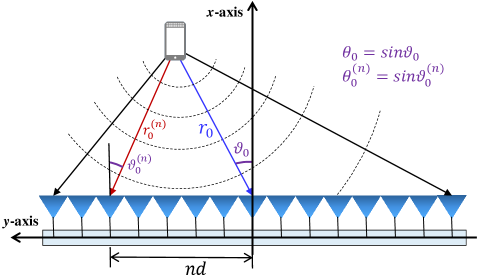
Due to the severe path loss incurred by the scatters, mmWave and THz communications heavily rely on the line-of-sight (LoS) path [4]. Therefore, we mainly focus on the near-field LoS channel, while the discussions in this paper can be straightforwardly extended to the non-LoS (NLoS) scenarios. As shown in Fig. 1, the user is located at with . Taking into account the near-field spherical wave characteristic [22], the channel between the -th BS antenna and the user at the -th subcarrier with and can be represented as
| (1) |
where denotes the wavenumber at subcarrier frequency and represents the distance between the user and the -th BS antenna. As the coordinate of the -th BS antenna is , can be derived from the geometry as . The path gain can be modeled as [23]
| (2) |
where wavelength and denotes the angle between the user and the -th BS antenna. Moreover, is the antenna gain and denotes normalized power radiation pattern, satisfying . An example of normalized power radiation pattern is [23]. Generally, the distance between the user and BS is larger than the array aperture . For example, for a 256-element ULA working at 30 GHz, is very likely to be larger than meters. With , we can assume based on the Fresnel approximation [24]. As a result, the near-field LoS channel can be represented as
| (3) |
where is the near-field array response vector.
Notice that since the near-field spherical wave characteristic is considered, the array response vector is significantly different from the classical far-field array response vector [25], where the latter is based on the planar wave assumption and ignores the influence of distance . The radius of the near-field region is determined by the Rayleigh distance [8]. For a 1-meter diameter array operating at 30 GHz, its Rayleigh distance reaches up to 200 meters. Therefore, in such a mmWave XL-MIMO system, the near-field spherical wave characteristic becomes essential and the distance information cannot be ignored.
However, since the distance is a complicated radical function with respect to the antenna index , it is difficult to analyze the property of the near-field spherical wavefront directly from (3). To deal with this problem, the Fresnel approximation [24] can be adopted to approximate as
| (4) |
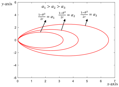
where is based on the second-order Taylor expansion . For expression simplicity, we denote and . As shown in Fig. 2, the curve corresponds to a ring in the physical space, and thus the curve is termed as distance ring . Then, according to (4), the -th element of can be approximated as
| (5) |
where denotes the -th element of vector . Since the residue phase in (5) has no relationship with the antenna index , we only need to focus on the vector .
II-B Near-Field Beam Split
At mmWave or THz band, frequency-independent PS-based beamformer is widely considered to serve the user by generating a focused beam aligned with location in the polar coordinate. Generally, the beamfocusing vector generated by frequency-independent PSs is usually set as to focus the beam energy on the location [26], where represents the array response vector (5) at frequency .
However, the array response vector (5) of the wideband channel is frequency-dependent, which mismatches the frequency-independent beamfocusing vector . This mismatch leads to the fact that, the beams generated by at different frequencies will be focused on different locations, which is detailed in the following Lemma 1.
Lemma 1.
For near-field wideband communications, the beam at frequency generated by will be focused on the location , satisfying
| (6) | ||||
| (7) |
where we define , , and .
Proof: At frequency , the array gain achieved by on an arbitrary user location with is
| (8) |
where we define . Apparently, the beam at frequency is focused on the location corresponding to the maximum array gain , i.e.,
| (9) |
where . Since and , it is obvious that is an optimal solution to maximize the function . Therefore, we have and , which leads to the results of (6) and (7).
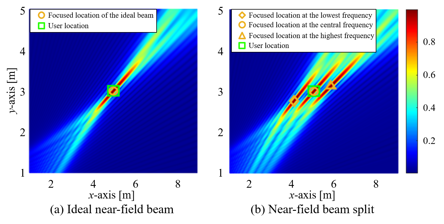
According to Lemma 1, the beam at is focused on the location . As shown in Fig. 3, since the desired user is located at , the beam at frequency cannot be aligned with the desired user location. This misalignment is termed as the “near-field beam split” effect [5], which will result in a severe array gain loss when is far away from in wideband XL-MIMO systems. For example, if the carrier frequency and bandwidth are GHz and GHz, and the BS is equipped with a 256-element ULA, then around 50% subcarriers will suffer from more than 50% array gain loss [5]. Therefore, the near-field beam split effect should be elaborately addressed, especially when the bandwidth is very large.
II-C Time-Delay Based Beamformer
To mitigate the near-field beam split effect, a method is to utilize TD based beamformer rather than PS based beamformer to generate frequency-dependent beams to match the frequency-dependent channels. Notice that the TD based beamsteering has been studied in the far-field wideband systems [12, 13, 14, 15, 16, 17, 18, 19], while in this study, we consider utilizing it to overcome and control the near-field beam split effect.
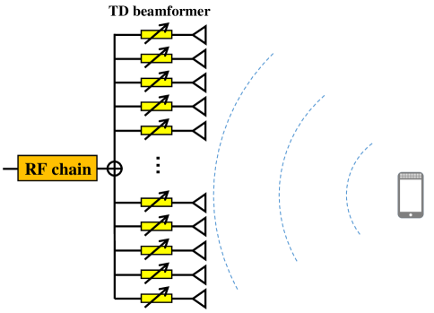
As shown in Fig. 4, we assume the BS is equipped with an -element TD beamformer111The main purpose of this paper is to derive that time-delay circuits are able to control the near-field beam split effect. Therefore, we directly utilize the time-delay beamformer as an example, while the discussion on some other low-power consumption architectures, such as delay-phase precoding, is left for future works.. Then the frequency response at frequency of the -th antenna is , where denotes the frequency-dependent beamforming vector, and denotes the adjustable time-delay parameter of the -th time-delay circuit. For expression simplicity, we denote as the adjustable distance, and then becomes . Notice that has a similar form with the array response vector . Thus, the -th adjustable distance can be set as , while and are adjustable delay parameters of a TD beamformer. Then, the corresponding beamfocusing vector at can be presented as
| (10) |
In this case, at frequency , the array gain on an arbitrary location with is given by
| (11) |
Obviously, the beam at is focused on . Similar to the derivation of the optimal solution of (9), approaches its maximum value when and . Therefore, the beam at frequency is focused on and , which is not relevant to . Then, once the LoS path information is available at the BS, and the delay parameters are set as and , then the beams across the entire bandwidth are able to be focused on the location and . As a consequence, the near-field beam split effect can be mitigated by the TD beamformer.
On the other hand, efficient wideband beamfocusing requires that the LoS path information is available at the BS side. To realize this requirement, in the following discussions, we prove that a TD beamformer can not only mitigate the near-field beam split effect, but also flexibly control its degree. Then, we will further utilize this property to achieve efficient near-field beam training to obtain .
III Mechanism of Near-Field Controllable Beam Split
In [17, 19, 18], the researchers proved the mechanism of far-field controllable beam split, i.e., by elaborately designing the time-delay parameters, the beams over the entire bandwidth are able to cover a desired angular range in the far-field. Taking advantage of this mechanism, multiple beams aligned with multiple angles can be generated by only one RF chain to acquire the far-field CSI rapidly. Similarly, to obtain the near-field CSI, we surprisingly find that time-delay circuits can not only control the angular coverage range but also control the distance coverage range of the beams, i.e., the near-field controllable beam split is achievable. In this section, we will prove the mechanism of this effect, and then in the next section utilize this mechanism to achieve fast near-field beam training. For readers better understand our ideas, we first prove the far-field controllable beam split and then extend it to the near-field scenarios.
III-A Far-Field Controllable Beam Split
For the far-field scenarios, the distances and are assumed to be larger than the Rayleigh distance RD, so that the spherical wavefront can be approximated as a planar wavefront. In this case, all of the distance-related parameters and reliably approach 0. Then, the array response vector becomes , and the beamfocusing vector realized by a TD beamformer becomes . Therefore, the array gain in (II-C) can be simplified as
| (12) |
where . It has been previously proved that the beams over the entire bandwidth generated by are focused on the spatial angle , with . However, notice that the spatial angle is corresponding to an actual physical angle as shown in Fig. 1, which implies the value range of is restrained by . By contrast, is an adjustable parameter of a TD beamformer. A question naturally arises that, if the adjustable parameter is set as , then what it has to do with the actual spatial angle ? Actually, the answer to this question is exactly the mechanism of the far-field controllable beam split.
For expression simplicity, parameter is termed as the abnormal value, while parameter is termed as the actual value. Restrained by the value range of , if is an abnormal value, it is obvious that . To acquire the relationship between and , we observe that the far-field array gain is a periodic function against with a period . For any integer , we have
| (13) |
In Section II, we have indicated that the optimal solution to maximize is . However, according to (13), we find that is just one of the optimal solutions for maximizing . The periodicity of implies that the optimal solutions should satisfy , . As a consequence, by solving , the focused spatial angle at frequency is derived as
| (14) |
where the function of is to ensure becomes an actual spatial angle. From (14), the mechanism of the far-field controllable beam split is acquired, which has the following features.
Feature 1: Since is an integer, if , the spatial angle is related to the frequency , which means beams at different frequencies will split towards different spatial angles. Therefore, despite the TD based beamsteering architecture being utilized, the far-field beam split effect can also be induced.
Feature 2: The specific value of is determined by . If belongs to the actual value range of , then can be zero and exactly equals to . That is to say, with , the far-field beam split effect is eliminated. While if becomes an abnormal value, then to guarantee that is an actual spatial angle, it is obvious that cannot be zero. For instance, if is set as , at the central frequency with , the corresponding spatial angle is , . Only if can be an actual spatial angle. Therefore, with , is not zero and thus is a function of the frequency , where the beam split effect is induced again.
Feature 3: Notice that the beam split pattern (14) of a TD beamformer is different from (6) of a PS beamformer. For a PS beamformer, the degree of beam split is fixed and uncontrollable. However, for a TD beamformer, the degree of beam split is controllable by adjusting . For instance, considering the central frequency , if is set as , then should be and . On the other hand, if is set as , then should be and . For the above two examples, although the spatial angles are the same, the integers are different, which indicates the degree of the beam split is different. Therefore, by adjusting the delay parameter , the integer is indirectly controlled, then the degree of beam split is adjusted. This property is termed as the far-field controllable beam split. Benefiting from this property, the adjustment on the angular coverage range of the beams is achieved, which can be utilized to realize fast far-field CSI acquisition [17, 19, 18].
In the next sub-section, we will extend this conclusion to a more general near-field scenario.
III-B Near-Field Controllable Beam Split
For the near-field scenario, the distances and are lower than the Rayleigh distance. Then and can not be zero, and the near-field spherical wave characteristics should be considered. To prove the mechanism of the near-field controllable beam split, analog to the derivation in the far-field scenarios, we consider the abnormal values for the adjustable parameters and in (10) simultaneously.
Specifically, it has been discussed before is an abnormal value for the angle. As for the distance-related parameter , since and , a realistic should be larger than zero. On this condition, is obvious the abnormal value for the distance ring. If and are actual values, it was proved in Section II-C that the near-field beam split effect is eliminated, i.e., beams are focused on and for all frequencies . On the other hand, for the abnormal value or , the following Lemma 2 explains the behaviors of the beams generated by .
Lemma 2.
If or , the beam at frequency generated by according to (10) will be focused on the location , satisfying
| (15) | ||||
| (16) |
where and are integers to guarantee and .
Proof: Similar to the derivation of (14), the periodicity of the near-field array gain function should be considered. It is proved in Appendix A that is a periodic function against the vector variable with a period . Therefore, for any integers and , can be rewritten as
| (17) |
It has been indicated in Section II that the optimal solution to maximize the array gain is . The periodicity in (17) implies is just one of the optimal solutions for maximizing . Besides, the optimal solutions should satisfy with and . Accordingly, to obtain the focused location of the beam at frequency by solving , we have and . As a consequence, and become and , respectively, where the function of integers and is to ensure that and are an actual spatial angle and an actual distance ring.
According to Lemma 2, the mechanism of the near-field controllable beam split is acquired, which has the following features.
Feature 1: If or , then or is related to the frequency , which means beams at different frequencies will be focused on different locations. Therefore, despite the TD beamformer being utilized, the near-field beam split effect can also be induced.
Feature 2: As the function of the abnormal value of has been discussed in the previous section, we mainly explain the impact of the abnormal value of on the integer here. If is an actual value, then could be zero, and for all beams, we have . However, if is an abnormal value, to guarantee , the value of must be larger than 0, and thus the beams at different subcarriers will be focused on different distances . For instance, let the delay parameter be , then we have . To guarantee is an actual distance ring, the integer should be larger than . Accordingly, when and , then the integer is enough to make and the beam at is focused on the distance ring . On the other hand, when and , then the integer is enough to make and the beam at is focused on the distance ring . As a consequence, the abnormal value of is able to introduce and control the beam split effect on the distance dimension.
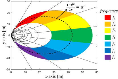
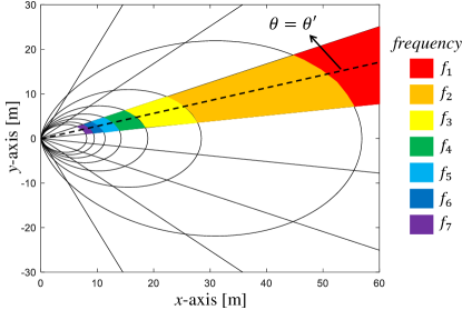
Feature 3: The far-field scenario is a special case of the near-field controllable beam split by setting . The far-field scenario assumes the distance is very large, and it can only control the beam split effect on the angle . By contrast, the near-field controllable beam split effect can adjust the degree of the beam split effect on the angle and distance jointly. For instance, one can set as an abnormal value and as an actual value, then we have , and . Therefore, the beam at frequency is focused on a location satisfying , which indicates that the beams are focused on multiple angles in the distance ring in the near-field, as shown in Fig. 5 (a). Moreover, we can set as an actual value and as an abnormal value, then the beams are focused on multiple distances at the same angle as shown in Fig. 5 (b), satisfying . As a result, by carefully designing the parameters and , the beams across the entire band could occupy multiple angles and distances simultaneously, and this property is more flexible than that in the far-field scenario.
In conclusion, the mechanism of near-field controllable beam split indicates that a TD beamformer can not only mitigate the near-field beam split effect, but also control its degree, i.e., one can flexibly adjust the covered angular range and distance range of the beams generated by TD beamformer over the entire bandwidth. A simple analogy of this effect is the dispersion of white light caused by a prism. Since a prism has different refractive indices for the wideband white light, the different frequency components of the pure light will disperse and eventually produce the rainbow. In our discussion, the function of time-delay circuits is similar to that of the prism. Therefore, the near-field controllable beam split effect is also termed as “near-field rainbow” in this paper.
By elaborately designing the pattern of the near-field rainbow as shown in Fig. 5, efficient near-field beam management can be realized, which will be discussed in the next section.
IV Proposed Beam Training Scheme
In this section, we first introduce the concept of near-field beam training and indicate the overhead for exhaustive near-field beam training is much larger than the far-field beam training, which is unacceptable in XL-MIMO systems. To solve this problem, we propose a wideband beam training algorithm by taking advantage of the near-field rainbow.
IV-A Exhaustive Near-Field Beam Training
Beam training is a well-adopted scheme to obtain CSI for current 5G systems [27]. The concept of near-field beam training can be derived from the classical far-field beam training. For the classical far-field beam training, the spatial angle information is desired. The optimal beamsteering vector for a user is selected from a predefined far-field beam codebook through a training procedure between the BS and the user. Generally, each codeword in the far-field codebook determines a unique spatial angle, where the distance is assumed to be very large so that the near-field property is ignored. Therefore, the entire far-field codebook occupies all of the potential angles in the far-field.
Similarly, the near-field beam training desires to obtain the location information of the dominant path between the BS and the user. The optimal beamfocusing vector is selected from a predefined near-field beam codebook through a training procedure between the BS and the user. Each near-field codeword determines a unique location, and the entire near-field codebook occupies all of the desired angles and distances.
To be more specific, we introduce the procedure of exhaustive near-field beam training realized by a TD beamformer. Notice that the procedure below is also valid for the PS beamformer when the bandwidth is not very large. We define as the potential range of spatial angle, satisfying . Moreover, we assume the minimum distance between the BS and the user is , so that the potential range of distance is or with . Then, multiple angles from and distances from are sampled simultaneously to construct the near-field codebook. As proved in [6], the sampled locations could satisfy
| (18) | ||||
| (19) |
where and . denotes the number of sampled angles and denotes the number of sampled distance rings. Notice that when , we have , and then the near-field codebook is naturally decayed to the far-field codebook. The exhaustive near-field beam training scheme searches the entire codebook and to obtain the optimal beamfocusing vector. Apparently, the overhead for exhaustive near-field beam training, i.e., the number of time slots used for beam training, is .
In the -th time slot, where with , , and , we set the parameters of the TD beamformer as and , and then generate the beamfocusing vector according to (10). Since and are actual values, the BS is able to transmit the pilot sequence to the user by the beam focused on the location . So the received signal in the -th time slot at is
| (20) |
where denotes the Gaussian noise, denotes the transmit power, and denotes the transmit pilot satisfying . After time slots, the estimated physical location corresponding to the largest user received power can be selected from the measured locations, where,
| (21) |
Finally, a near-field beam aligned with the location can be generated to serve the user, and a near-optimal beamfocusing gain can be achieved.
Nevertheless, since the exhaustive near-field beam training scheme has to search the entire near-field codebook exhaustively, and the scale of the near-field codebook is much larger than that of the far-field, i.e. , the training overhead is unacceptable in practice. Therefore, a near-field beam training scheme with low pilot overhead is essential for XL-MIMO systems.
IV-B Proposed Near-Field Beam Training Scheme
The main reason for the high training overhead of exhaustive near-field beam training is that only one physical location can be measured in each time slot. By contrast, as we discussed in Section III-B, a TD beamformer is able to generate multiple beams focusing on multiple locations by only one RF chain. Taking advantage of the near-field rainbow, multiple physical locations can be measured simultaneously in each time slot. Inspired by this observation, we propose a near-field rainbow-based beam training method to significantly reduce the training overhead.
Generally, since the spatial resolution of an antenna array on the angle is much higher than that on the distance, the number of sampled angles is usually much larger than the number of sampled distances [6]. Thus, the training overhead is mainly determined by the search of angle . Therefore, the near-field rainbow on the angle dimension, as shown in Fig. 5 (a), is utilized to avoid the exhaustive search of angle, i.e., the angle-related parameters are set as abnormal values, while the distance-related parameters can be set as actual values. In other words, the proposed scheme searches the optimal angle in a frequency division manner, and searches the optimal distance ring in a time division manner. The specific procedure of the proposed beam training scheme is illustrated in Algorithm 1.
Firstly, in steps 1-2, we desire to design the abnormal parameter , so that the frequency-dependent angles across the entire band is able to cover the entire potential angle range , as shown in Fig. 5 (a). To realize this target, we first assume that, at the central frequency , the beam is aligned with the angle , where is a predefined spatial angle satisfying . Then we have
| (22) |
Without loss of generality, we assume the delay parameter , then is a positive integer. In this case, the frequency-dependent angle is monotonically decreasing with respect to the frequency .
Moreover, since the available bandwidth is , the lowest frequency and the highest frequency are and , respectively. Therefore, the minimum and maximum values of are and , respectively. To cover the entire potential angles , it should satisfy
| (23) | ||||
| (24) |
By solving (22), (23), and (24), one of the solutions to is
| (25) |
where denotes the nearest integer greater than or equal to , and is given by .
Then, in step 4, different distance rings are searched in different time slots by adjusting the normal delay parameter . Similar to the exhaustive near-field beam training scheme, the potential range of distance ring is , and the number of distance rings to be measured is . Therefore, in the -th time slot, is set as with to measure the beamfocusing gains on the distance ring .
As a result, with the parameters and , as shown in Fig. 5 (a), the beams generated in step 5 by the TD beamformer is able to occupy the entire angular range in the distance ring . Utilizing these beams, in step 6, the received signal in the -th time slot at frequency is denoted as
| (26) |
where . The optimal beamfocusing vector is corresponding to the maximum beamfocusing gain . Since and , the maximum likelihood estimation of is
| (27) |
Thus, the beamfocusing gain can be estimated as . Based on the definition of in Section II, we have , where is a constant that is not relevant to . Notice that the proposed beam training scheme does not require the specific value of . As long as the relationship between and is available, whether quadratic function, exponential function, and so on, the proposed scheme is always valid.
Besides, in step 8, based on the formulation of beamfocusing gain , the label of the optimal beam and is acquired by maximizing over the total measured distance rings and subcarriers, where
| (28) |
Eventually, in steps 9-10, based on the mechanism of the near-field rainbow (15), the estimated spatial location is
| (29) | ||||
| (30) |
After that, the beam training is completed, and the BS can generate the beamfocusing vector to serve the user for data transmission.
The advantage of the proposed near-field rainbow based beam training method is that the optimal angle is searched out in a frequency division manner. Therefore, the training overhead is only determined by the overhead for searching the optimal distance ring, which is significantly reduced. In the next sub-section, we quantitatively analyze the training overheads of the two near-field beam training schemes above.
IV-C Comparison on the Beam Training Overhead
Beam training overhead refers to the number of time slots used for beam training. It is obvious that, the training overhead of the exhaustive near-field beam training scheme is , while the training overhead of the proposed near-field rainbow based scheme is . As discussed in [6], the number of distance rings is generally much less than the number of angles. For instance, if the BS antenna number is , the carrier is GHz, and the minimum distance is m, then is usually set as while is generally set as 10 [6]. In this case, the training overhead is much less than . Therefore, benefiting from the near-field rainbow, the proposed scheme is able to significantly reduce the pilot overhead for near-field beam training, which will be further verified by simulation results in Section V.
V Simulation Results
In this section, simulations are provided to verify the effect of the near-field rainbow and demonstrate the performance of the proposed near-field rainbow based beam training scheme. We consider a wideband XL-MIMO system, where the BS equips an -element ULA with a TD beamformer. The carrier frequency is GHz, the number of sub-carriers is , and the bandwidth is GHz.
V-A The Demonstration of Near-Field Controllable Beam Split
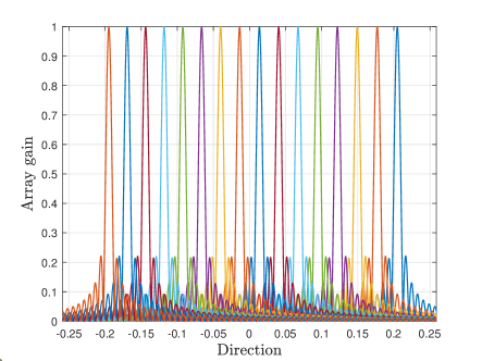
Firstly, in Fig. 6, we verify that time-delay circuits are able to produce near-field controllable beam split. Specifically, in Fig. 6 (a), the near-field rainbow on the dimension of angle is evaluated. We set the delay parameter as and the parameter as with m. On the distance ring , the array gains at different frequencies with respect to (w.r.t) the angle are shown in Fig. 6 (a). For clarity, only a few frequencies are plotted. The beams over different frequencies are focused on multiple angles in the distance ring , and cover a given angular range . Therefore, the near-field rainbow on the angle dimension is verified.
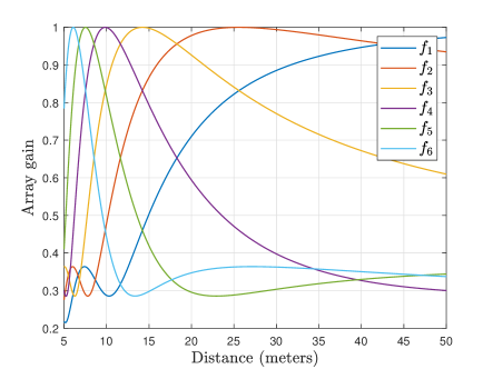
Then, in Fig. 6 (b), the near-field rainbow on the dimension of distance is evaluated. We set the angle as and the distance ring as . In the physical angle , the array gains at different frequencies w.s.t the distance are shown in Fig. 6(b). For clarity, only a few frequencies are plotted. The beams over different frequencies are focused on multiple distances in the angle , which covers the entire distance range. Therefore, the near-field rainbow on the distance dimension is also achievable.
V-B Beam Training Performance
In this subsection, the performance of the proposed near-field rainbow based beam training scheme is evaluated. The potential spatial angle range of the user is set as , while the potential distance of the user is set as and thus the range of is . The spatial angle at the center frequency is fixed to . Then, for the proposed near-field rainbow based scheme, according to (25), the delay parameter is acquired as with . Moreover, we set the number of distance rings to be searched as . For the exhaustive near-field beam training, the number of angles to be searched is . Finally, we use the average rate performance to quantify the beam training performance, which is mathematically defined as
| (31) |
where denotes the beamfocusing vector for data transmission searched by beam training and SNR denotes the signal-to-power ratio. The compared benchmarks are shown below.
-
•
Perfect CSI: The perfect channel is available at the BS, which is served as the benchmark for the upper bound of average rate performance.
-
•
Far-field rainbow based beam training: The classical wideband far-field beam training scheme achieved by TD beamformer in [18]. This method can be regarded as the far-field rainbow-based beam training scheme, where only the optimal angle is searched in a frequency-division manner and the distance ring is assumed to be zero.
-
•
Near-field hierarchical beam training: This method is the hierarchical beam scheme training designed for reconfigurable intelligence surface (RIS) aided near-field communications [21]. We transform this method to XL-MIMO scenarios for comparison.
-
•
Far-field hierarchical beam training: This method is the classical hierarchical beam training designed for the far-field scenarios [20].
-
•
Exhaustive search: This method is the exhaustive near-field beam training scheme provided in Section IV-A. In the training procedure, we first fix the distance ring and exhaustively search all of the angles . Then, we change the distance ring and repeat the above steps until all of the distance rings and angles are measured.
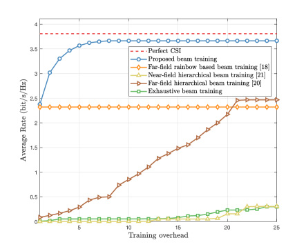
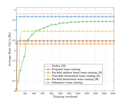
Fig. 7 illustrates the average rate performance against the training overhead. The training overhead is increasing from 0 to . The SNR is set as 10 dB. realizations of the user location are generated for Monte Carlo simulations, where and . In the -th time slot, we utilize the optimal beamforming vector searched during the time slots to serve the user. Specifically, the training overhead of the two far-field schemes are both very low, e.g., 22 overhead for the hierarchical far-field scheme and only one overhead for the far-field rainbow based scheme. However, since the far-field schemes only consider the angle information while ignoring the distance information, their average rate performance is not satisfactory. Besides, to achieve a satisfactory average rate, the training overhead of the near-field hierarchical scheme and the exhaustive scheme will be very high, e.g., 200 overhead for the near-field hierarchical scheme and more than 1000 for the exhaustive scheme. By contrast, the proposed near-field rainbow based beam training scheme enjoys a much higher average rate performance with very low overhead. This is thanks to two factors: 1) both the angle and distance information are considered, 2) the near-field rainbow effect is exploited to avoid the exhaustive search for the angle information. Actually, the proposed scheme has already achieved 96% of the average rate benchmark with only 8 training overhead.
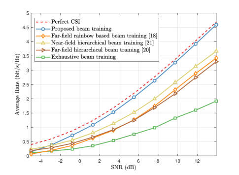
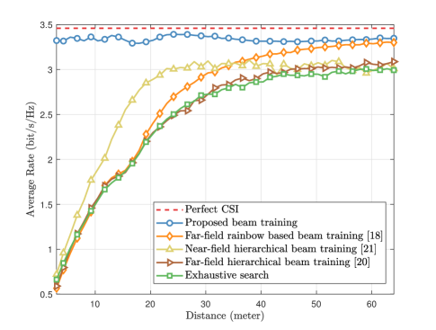
Fig. 8 shows the impact of SNR on different beam training schemes. Here, the SNR is increasing from -5 dB to 15 dB. The maximum training overhead for all considered methods is set as . Notice that in our simulations, only the overhead for exhaustive beam training is , while the overhead for other schemes is set according to their overhead requirements as illustrated in Fig. 7, which are always less than . The other simulation settings are the same as those in Fig. 7. It is clear from Fig. 8 that, the proposed scheme outperforms all existing far-field and near-field beam training schemes, and is able to achieve the near-optimal achievable average rate performance compared with the benchmark. In addition, we can observe that the exhaustive beam training scheme suffers from severe degradation of the average rate performance. This is mainly because the maximum training overhead (256) is much less than the required training overhead (more than 1000) for the exhaustive scheme to achieve satisfactory average rate performance.
In Fig. 9, we illustrate the average rate performance against the distance. Here, the distance between the user and BS is gradually increasing from 3 meters to 60 meters. The parameters are set as follows: dB, , . The other simulation settings are the same as those in Fig. 8. The impact of near-field propagation on the beam training performance is clear in Fig. 9. For the far-field schemes, with the decrease of distance, near-field propagation becomes dominant and thus the average rate of these far-field schemes rapidly deteriorates. As for the degradation of the exhaustive scheme, since the maximum training overhead is limited to 256, this scheme is hard to search the locations in the near-field. Moreover, although the near-field hierarchical beam training scheme is able to slightly alleviate the average rate loss, its performance is unacceptable when the distance is less than 20 meters. By contrast, since the proposed scheme is able to search the optimal angle and distance with very low pilot overhead by exploiting the near-field rainbow, its performance is robust to all considered distances, whether in the near-field or in the far-field.
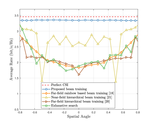
Fig. 10 shows the average rate performance against the angle . Here, the angle is gradually increasing from to and the distance is randomly generated from . The other simulation settings are the same as those in Fig. 9. Notice that although the distance is fixed, the distance ring still varies with the angle . For the far-field schemes, their performance is severely degraded when the angle is around zero. This is because the near-field property is more significant when the angle is around zero, which has been proved in [5]. Moreover, there exists severe fluctuation for the near-field hierarchical beam training scheme. This is because the near-field hierarchical scheme proposed in [21] creates the near-field codebook by uniformly sampling the codeword in the cartesian coordinates. It has been indicated in [6] that this kind of codebook cannot realize satisfactory beam training performance in the entire near-field environment. By contrast, the proposed scheme achieves a near-optimal average rate for all considered angles.
VI Conclusions
This paper investigated the wideband near-field beam training for XL-MIMO systems. The mechanism of the near-field rainbow is revealed, i.e., time-delay circuits can flexibly control the degree of the near-field beam split effect. Then, a near-field rainbow based beam training scheme was proposed to search the optimal angle in a frequency-division manner, and the optimal distance is searched in a time-division manner. The simulation results verified that: i) the beams generated by a TD beamformer over the entire bandwidth can cover multiple angles and distances, ii) our near-field rainbow based scheme can achieve a near-optimal average rate with much-reduced training overhead, iii) the performance of our scheme is robust to the distance and angle. This paper unveiled that although the near-field beam split effect induces a severe beamfocusing gain loss, it also provides a new possibility to realize fast near-field CSI acquisition. In our future work, we will extend the mechanism of the near-field rainbow to other beamforming architectures, such as the delay-phase precoding architecture [15].
Appendix A. The Periodicity of
is a periodic function against the vector variable with period . Specifically, for any integers and , we have
| (32) |
Since is an integer multiple of , we have . Therefore,
| (33) |
As a result, the periodicity of function is proved.
References
- [1] E. D. Carvalho, A. Ali, A. Amiri, M. Angjelichinoski, and R. W. Heath, “Non-stationarities in extra-large-scale massive MIMO,” IEEE Wireless Commun., vol. 27, no. 4, pp. 74–80, Aug. 2020.
- [2] P. Frenger, J. Hederen, M. Hessler, and G. Interdonato, “Improved antenna arrangement for distributed massive MIMO,” 2017. [Online]. Available: patentscope.wipo.int/search/en/WO2018103897
- [3] T. S. Rappaport, Y. Xing, O. Kanhere, S. Ju, A. Madanayake, S. Mandal, A. Alkhateeb, and G. C. Trichopoulos, “Wireless communications and applications above 100 GHz: Opportunities and challenges for 6G and beyond,” IEEE Access, vol. 7, pp. 78 729–78 757, Jun. 2019.
- [4] H. Elayan, O. Amin, B. Shihada, R. M. Shubair, and M. Alouini, “Terahertz band: The last piece of RF spectrum puzzle for communication systems,” IEEE Open J. Commun. Society, vol. 1, pp. 1–32, Nov. 2020.
- [5] M. Cui, L. Dai, R. Schober, and L. Hanzo, “Near-field wideband beamforming for extremely large antenna array,” arXiv preprint arXiv:2109.10054, Sep. 2021.
- [6] M. Cui and L. Dai, “Channel estimation for extremely large-scale MIMO: Far-field or near-field?” IEEE Trans. Commun., vol. 70, no. 4, pp. 2663–2677, Apr. 2022.
- [7] H. Zhang, N. Shlezinger, F. Guidi, D. Dardari, M. F. Imani, and Y. C. Eldar, “Beam focusing for near-field multi-user mimo communications,” IEEE Trans. Wireless Commun., pp. 1–1, Mar. 2022.
- [8] K. T. Selvan and R. Janaswamy, “Fraunhofer and fresnel distances: Unified derivation for aperture antennas,” IEEE Antennas Propag. Mag., vol. 59, no. 4, pp. 12–15, Aug. 2017.
- [9] M. Cui, Z. Wu, Y. Lu, X. Wei, and L. Dai, “Near-field communications for 6G: Fundamentals, challenges, potentials, and future directions,” arXiv preprint arXiv:2203.16318, Mar. 2022.
- [10] O. E. Ayach, S. Rajagopal, S. Abu-Surra, Z. Pi, and R. W. Heath, “Spatially sparse precoding in millimeter wave MIMO systems,” IEEE Trans. Wireless Commun., vol. 13, no. 3, pp. 1499–1513, Mar. 2014.
- [11] S. Mumtaz, J. Rodriquez, and L. Dai, MmWave Massive MIMO: A Paradigm for 5G. Academic Press, Elsevier, 2016.
- [12] H. Hashemi, T. Chu, and J. Roderick, “Integrated true-time-delay-based ultra-wideband array processing,” IEEE Commun. Mag., vol. 46, no. 9, pp. 162–172, Sep. 2008.
- [13] E. Ghaderi, A. Sivadhasan Ramani, A. A. Rahimi, D. Heo, S. Shekhar, and S. Gupta, “An integrated discrete-time delay-compensating technique for large-array beamformers,” IEEE Trans. Circuits Syst. I, Reg. Papers, vol. 66, no. 9, pp. 3296–3306, Sep. 2019.
- [14] C. Lin, G. Y. Li, and L. Wang, “Subarray-based coordinated beamforming training for mmWave and sub-THz communications,” IEEE J. Sel. Areas Commun., vol. 35, no. 9, pp. 2115–2126, Sep. 2017.
- [15] L. Dai, J. Tan, Z. Chen, and H. Vincent Poor, “Delay-phase precoding for wideband THz massive MIMO,” IEEE Trans. Wireless Commun., Mar. 2022.
- [16] D. Q. Nguyen and T. Kim, “Joint delay and phase precoding under true-time delay constraint for THz massive MIMO,” arXiv preprint arXiv:2111.10365, Nov. 2021.
- [17] H. Yan, V. Boljanovic, and D. Cabric, “Wideband millimeter-wave beam training with true-time-delay array architecture,” in Proc. 2019 53rd Asilomar Conference on Signals, Systems, and Computers, 2019, pp. 1447–1452.
- [18] V. Boljanovic, H. Yan, C.-C. Lin, S. Mohapatra, D. Heo, S. Gupta, and D. Cabric, “Fast beam training with true-time-delay arrays in wideband millimeter-wave systems,” IEEE Trans. Circuits Syst. I, Reg. Papers, vol. 68, no. 4, pp. 1727–1739, Apr. 2021.
- [19] J. Tan and L. Dai, “Wideband beam tracking in THz massive MIMO systems,” IEEE J. Sel. Areas Commun., vol. 39, no. 6, pp. 1693–1710, Jun. 2021.
- [20] S. Noh, M. D. Zoltowski, and D. J. Love, “Multi-resolution codebook and adaptive beamforming sequence design for millimeter wave beam alignment,” IEEE Trans. Wireless Commun., vol. 16, no. 9, pp. 5689–5701, Sep. 2017.
- [21] X. Wei, L. Dai, Y. Zhao, G. Yu, and X. Duan, “Codebook design and beam training for extremely large-scale RIS: Far-field or near-field?” China Commun., Jun. 2021.
- [22] Z. Zhou, X. Gao, J. Fang, and Z. Chen, “Spherical wave channel and analysis for large linear array in LoS conditions,” in Proc. IEEE Globecom Workshops, Dec. 2015, pp. 1–6.
- [23] W. Tang, M. Z. Chen, X. Chen, J. Y. Dai, Y. Han, M. Di Renzo, Y. Zeng, S. Jin, Q. Cheng, and T. J. Cui, “Wireless communications with reconfigurable intelligent surface: Path loss modeling and experimental measurement,” IEEE Trans. Wireless Commun., vol. 20, no. 1, pp. 421–439, Jan. 2021.
- [24] J. Sherman, “Properties of focused apertures in the Fresnel region,” IRE Trans. Antennas Propag., vol. 10, no. 4, pp. 399–408, Jul. 1962.
- [25] D. Tse and P. Viswanath, Fundamentals of Wireless Communication. Cambridge, U.K.: Cambridge Univ. Press, 2005.
- [26] D. Headland, Y. Monnai, D. Abbott, C. Fumeaux, and W. Withayachumnankul, “Tutorial: Terahertz beamforming, from concepts to realizations,” APL Photonics, vol. 3, p. 051101, May 2018.
- [27] W. Wu, D. Liu, X. Hou, and M. Liu, “Low-complexity beam training for 5G millimeter-wave massive MIMO systems,” IEEE Trans. Veh. Technol., vol. 69, no. 1, pp. 361–376, Jan. 2020.