Near Heisenberg limited parameter estimation precision by a dipolar Bose gas reservoir engineering
Abstract
We propose a scheme to obtain the Heisenberg limited parameter estimation precision by immersing atoms in a thermally equilibrated quasi-one-dimensional dipolar Bose-Einstein condensate reservoir. We show that the collisions between the dipolar atoms and the immersed atoms can result in a controllable nonlinear interaction through tuning the relative strength and the sign of the dipolar and contact interaction. We find that the repulsive dipolar interaction reservoir is preferential for the spin squeezing and the appearance of an entangled non-Gaussian state. As an useful resource for quantum metrology, we also show that the non-Gaussian state results in the phase estimation precision in the Heisenberg scaling, outperforming that of the spin-squeezed state.
pacs:
I introduction
One of main goals of quantum metrology is to achieve parameter (or phase) estimation precision beyond the shot-noise limit Caves1981 ; Yurke1985 ; Holland1993 ; Giovannetti2011 ; Dorner2009 ; Sanders1995 ; Ma2011 ; Ma2011B ; Humphreys2013 ; Dowling2008 ; Lvovsky2009 . Atomic spin squeezed states (SSSs) play an important role in quantum phase estimation and have been widely studied Kitagawa1993 ; Wineland1994 ; Momer ; Sorensen2001 ; Poulsen2001 ; Jin2009 ; Jin2010 ; Guehne2009 ; Wang2003 ; Liu2011 in the past few decades ever since the pioneer work of Kitagawa and Ueda Kitagawa1993 , who showed that the SSSs can be dynamically generated from the so-called one-axis twisting interaction (OAT) among spin- particles bou ; kas . As useful quantum resource, the SSSs have been proposed to achieve such a sub-shot-noise limited phase sensitivity Wineland1994 ; Momer ; Sorensen2001 ; Poulsen2001 ; Jin2009 ; Jin2010 ; Guehne2009 ; Wang2003 ; Liu2011 . Recently, Stroble et al. strobel experimentally demonstrated that the OAT can also generate entangled non-Gaussian states (ENGSs), which can outperform the spin-squeezed state. The OAT interaction have been proposed and demonstrated using ion traps Momer , Rydeberg atoms macri , nitrogen-vacancy centers Bennett and atomic Bose-Einstein condensates (BECs).
BECs due to their unique coherence properties and the controllable nonlinearity bou ; kas , have attracted much attention for quantum metrology. Experimental realizations of the OAT model has been proposed and demonstrated through Feshbach resonances gros or spatially separating the components of BECs rie . Besides, the atomic BECs also often as the reservoirs suitable for engineering is considered widely Palzer ; Will ; Cirone ; Spethmann ; Scelle ; Zipkes ; Schmid ; Balewski ; Recati ; Ng ; bargill ; Bru . For instance, one can drastically enhance the OAT interaction by placing a two-state condensate in a completely different special BEC reservoir bargill .
So far, the studies of bosonic atoms for metrology are mainly focused on -wave contact interaction. However, for ultracold atoms there also exists long-rang magnetic dipole-dipole interaction (MDDI) yi2000 ; Goral2002 ; yi ; yi2007 ; lu2 . In experiments, dipolar BECs have been realized for atoms with large magnetic dipole moments Lu ; Aikawa . Furthermore, both the sign and the strength of the effective dipolar interaction can be tuned via a fast rotating orienting field Giovanazzi ; Griesmaier2006 ; Lahaye . Very recently, Yuan et al. have used the quasi-2D dipolar BEC as reservoir engineering to study the non-Markovian dynamics of an impurity atom yuan . Therefore, the effects of the MDDI should be considered in the realizations of the OAT model based on dipolar BEC.
In this paper, we realize the OAT model induced by the reservoir dephasing noise, which has been widely viewed as one of the main obstacles for quantum metrology. We consider the dynamics of two-mode BEC consisting of atoms coupled to a one-dimensional (1D) dipolar Bose gas reservoir. It show that, the collisions interaction between the dipolar BEC reservoir and the immersed atoms can be described by a spin-boson model. Through calculating the SS , and the quantum Fisher information (QFI) , we find that the dephasing noise can produce SSSs and ENGSs. And the degree of the SS and entanglement both depends on the relative strength and sign of the dipolar and contact interaction. In other words, the repulsive dipolar interaction reservoir can induce better SS and ENGSs. Compared with spin squeezed states, ENGSs can last for a very long time under the dephasing noise. It can monotonically increase in the regimes without SS (), next successively undergoes metastable entangled states and entanglement suddenly increase, corresponding to and , respectively. According to Cramér-Rao theorem, , we know that means that the states are entangled and useful for sub-shot-noise-limited phase-estimation precision; and is the maximal entangled states, corresponding to the Heisenberg limit. This confirms that the phase estimation sensitivity can approach to Heisenberg limit, when using ENGSs for metrology.
The paper is organized as follows. In Sec. II, we give the model of immersed atoms interacting with the thermally equilibrated quasi-1D dipolar BEC reservoir. In Sec. III, we study the dynamics evolution of the atoms due to the dephasing noise. The SS and entanglement dynamical behaviors are discussed in Sec. IV and Sec. V. Finally, we draw our conclusion in Sec. VI.
II formulation
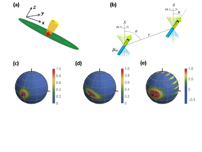
We consider a system of two states atoms with up and down states immersed in a quasi-1D dipolar gas reservoir. And the system atoms are confined in a harmonic trap that is independent of the internal states [see Fig.1(a)]. In general, the interaction between the system atoms and the reservoir is described by the Hamiltonian
| (1) |
where is the two-state atomic Hamiltonian, is the dipolar gas reservoir Hamiltonian, and describes their interaction.
II.1 Two level atom system
The spin Hamiltonian provides the most intuitive description in the internal case of two-mode trapped atomic BEC
| (2) |
Here, we define the pseudo-spin operator based on space orbitals as , where is the Pauli matrices, and denotes the annihilation operators of the atom states. The energy difference of the two states and nonlinearity depend on the mean filed wave-function of the two modes. We assume that the two modes have the same spatial orbital
| (3) |
where with being the trap frequency, and being the mass of atom. Therefore, with coupling constants and being -wave scattering length. For and the chosen hyperfine states, are almost equal: and , with being the Bohr radius. Then, the nonlinearity is close to zero. We point out that is tunable via Feshbach resonance, but the price of these methods is significantly increased atom losses bargill . Below, we choose and apply a dipolar gas reservoir to induce a stronger nonlinearity interaction.
II.2 Bogoliubov modes of quasi-1D dipolar gas reservoir
In second-quantized form, the many-body Hamiltonian of the 1D dipolar BEC is
| (4) | |||||
where is the field operator and is the single-particle Hamiltonian with being the mass of the atom. Here, we have assumed that the dipolar BEC to be confined in a cylindrically symmetric trap with a transverse trapping frequency and negligible longitudinal confinement along the direction, i.e., . In three dimensions, the two-body interaction is
| (5) |
where the contact interaction strength is with being the -wave scattering length; the dipolar interaction strength is , where is a length scale characterizing the MDDI with the vacuum permeability, the magnetic dipole moment; here is a unit vector.
To obtain the effective 1D interaction potential, , in Hamiltonian (4). We assume that the transverse wave function of all the reservoir atoms is
| (6) |
with being the width of the Gaussian function. By integrating out the and variables, we can obtain the Fourier transform of the 1D interaction potential (as shown in Appendix A)
| (7) |
with , where
| (8) |
with being the incomplete Gamma function.
To proceed, in the degenerate regime, the bosonic field can be decomposed as
| (9) |
with being the condensate linear density, the length of the reservoir, () the annihilation (creation) operators of the Bogoliubov modes with momentum . And its Bogoliubov modes are
| (10) |
with being the free-particle energy. Where the excitation energy is Cirone
| (11) | |||||
with dimensionless parameters . Hence, the Hamiltonian for the collective excitations is
| (12) |
The sum over Bogoliubov modes exclude the zero mode and will act as the reservoir under our model.
II.3 Interaction Hamiltonian
We assume that the reservoir atoms are coupled with the up state of the system atoms via a Raman transition Cirone ; yuan
| (13) |
where with the atoms and reservoir scattering length and reduced mass By substituting Eqs. (3) and (9) into the above interaction Hamiltonian and omitting the square terms about and , we have
| (14) |
where
| (15) | |||||
and
| (16) |
III System dynamical evolution
In the interaction picture with respect to , the total Hamiltonian is
| (17) |
which is a non-Hermitian dephasing spin-boson model with being the up state number operator. Here the non-Hermitian term is phenomenally introduced to describe the one-boby particle loss rate, owing to inelastic collisions between the system atoms and the noncondensed thermal atoms. It results in the particles be kicked out from the system. Such a kind of loss is a typical dissipation effect and has been widely studied strobel ; pawlowski ; hao ; spehner ; huang .
By using of Magnus expansion bargill , the time evolution operator can be read as where the effective Hamiltonian is (see Appendix B for details)
| (18) |
with and . From the above equation, we can find that the collisional interaction between the atoms and reservoir induce a nonlinear term , corresponding to the OAT Hamiltonian, and the noise induced nonlinear strength is Breuer
| (19) |
Here, the reservoir spectral density defined as . In the continuum limit, , we have
| (20) | |||||
where with being the roots of the equation and the dimensionless parameter is
| (21) |
Assuming that the initial state of the total system is given by
| (22) |
where is CSS, with the probability amplitudes and total spin for a system consisting of condensated atoms. And the density matrix of reservoir read as
| (23) |
with the inverse temperature. With the help of Eq. (18), the time-evolution reduced matrix elements of the atom system at any later time is found by tracing over the reservoir degrees of freedom
| (24) | |||||
with decoherence function
| (25) |
which is a function of temperature .
In Eq. (24), and , respectively, correspond to the unitary and non-unitary evolution due to the effects of the reservoir. Equations (19) and (25) show that both and depend on the reservoir spectral density , which can be controlled by tuning the MDDI of the dipolar Bose gas reservoir Giovanazzi ; Griesmaier2006 ; Lahaye . This is the main difference from Feshbach resonances method whose control is on the system atoms directly and will strongly enhance three-body loss near resonances regime beside the one-body loss. Therefore, in our model the one-body particle loss due to the inelastic collisions of the noncondensed atoms maybe the main loss mechanism that need considering. When temperature is low enough the values of one-body loss rate will be very small, since there is only a small number of thermal atoms with sufficient energy to knock atoms out of condensate Dalfovo . For simplicity, hereafter we only consider the case of , and choose as a free parameter.
IV Spin squeezing and entangled non-Gaussian spin states
IV.1 Spin squeezing parameter
Now, a state is regarded as squeezed if the variance of one spin component normal to the mean spin vector is lower than the Heisenberg limited value. The SS parameter defined by Wineland is Wineland1994
where represents the minimal variance of the spin component perpendicular to the mean spin direction . Where the mean spin is . A state is spin squeezed if . In addition, the smaller is, the stronger the squeezing is. If , the squeezing parameter can be evaluated explicitly
| (26) |
which does not depend on . And the optimally squeezed direction is , with
| (27) |
When considering the one-body losses, the form of SS has given in Appendix A.
Equation (26) indicates that the dephasing noise plays two different roles: On one hand, it can generate the SS by creating the nonlinear interaction ; on the other hand, it degrades the degree of SS via the decoherence function .
IV.2 QFI and entanglement of non-Gaussian spin states
To investigate the entanglement created by the dipolar BEC reservoir, we can also introduce the QFI. In general, the states that are entangled and useful for sub-shot-noise-limited parameter-estimation precision is identified by the QFI criterion . The QFI with respect to , acquired by an SU(2) rotation, can be described as Ma2011B
| (28) |
where with being the optimal rotation direction, and the matrix element for the symmetric matrix is
| (29) |
with being the eigenvalues (eigenvectors) of .
For simplicity, we first consider the case of small , e.g., . When setting and neglecting the particle loss, e.g., , the QFI can be calculated analytically
| (30) |
with
| (31) |
in -axis direction, and
| (32) |
in plane, which can also be obtained by using of Eq. (29) (see Appendix B).
The maximal QFI can be found in axis direction
| (33) |
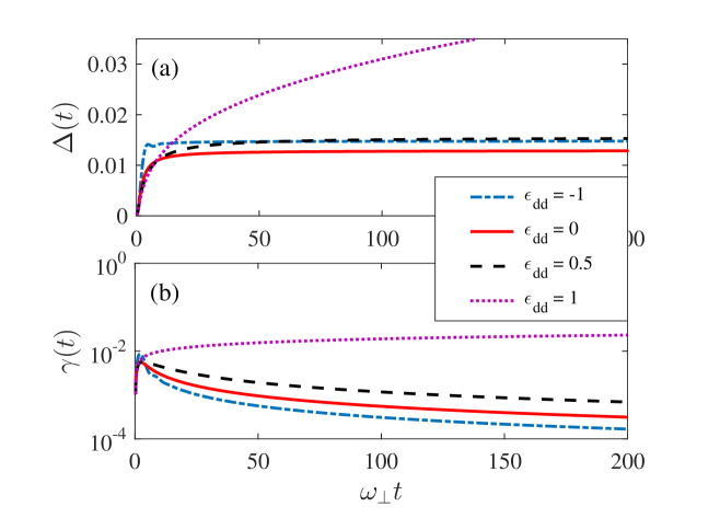
when choosing optimal interrogation time . Equation (33) reveals that the values of is directly related to the QFI. One finds (the Heisenberg limit) if . Fortunately, Fig. 2(b) indicates that the nearly neglectable can be obtained when the dipolar Bose gas reservoir with repulsive MDDI. Therefore, the main limitation of Heisenberg scaling is one-body loss mechanism in our scheme. Next, we consider large and the case of numerically.
V Results and discussion
As a concrete example, we consider a BEC reservoir of atoms, for which we have and with the Bohr magneton. This means that and dipolar interaction is mainly attractive since then the attraction is stronger than the short-range repulsion. However, not only the contact interaction strength can be tunable via Feshbach resonance, but also both the sign and the strength of the effective dipolar interaction can be tuned by the use of a fast rotating orienting field. Later, we will consider the values of , which is repulsive (attractive) MDDI for ().
Numerically, it is convenient to introduce the dimensionless units: for energy, for time, and for length. To obtain the values of dimensionless parameter and , we assume a quasi-1D trap with and ; and the corresponding harmonic oscillator width is . We assume that the linear density of the quasi-1D condensate is , and the -wave scattering length between Rb and Dy atoms is yuan . Then, we shall take and in the results presented below.
Since both the SS and QFI depend on and let us first investigate the time dependence of dephasing factor. From Fig. 2, we can clearly see that the squeezing rate is nearly constant, . Whereas is decreasing with time, what is more we can get very small (e.g.) when . Comparing and , we can also find that the values of (squeezing rate) is larger than (dispersive rate) for , which means that we can obtain strong squeezing and large QFI by the reservoir’s engineering with repulsive MDDI.
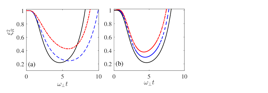
In Fig. 3, we plot the SS dynamics of two-mode BEC consisting atoms coupled to a 1D dipolar Bose gas reservoir for various values. As is shown in Fig. 3(a), the optimal squeezing can be achieved within short time scale, and after a transient time, it is lost () and then ENGSs are produced. However, for repulsive-dipolar-interaction reservoir, we can obtain stronger SS, due to their smaller dispersive rate . In Fig. 3(b), we further plot the time evolution of for various atom loss rates. It indicates that the squeezing degree degraded with the increasing of the atom loss rate.
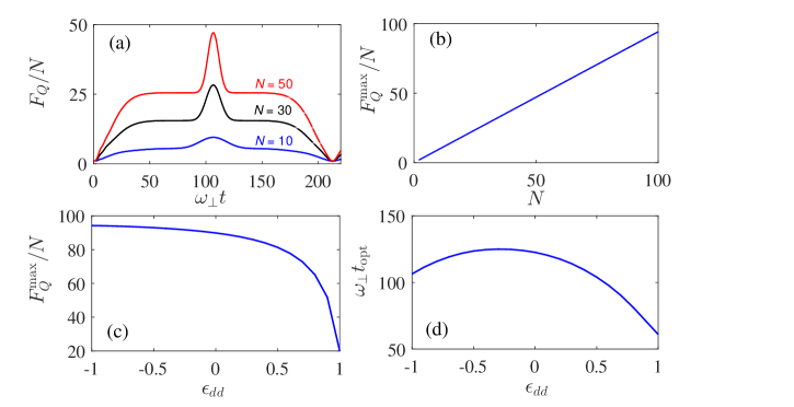
Figure 4 illustrates the QFI amplification rates with respect to the initial state (CSS) . In Fig. 4(a), we present the time dependence of QFI amplification rates with repulsive interaction. We see that differ from the case of SS, the amplified QFI can last for a very long time, which means that the ENGSs can be produced and achieve the maximal even in the regimes without squeezing. The optimal QFI first monotonically increasing and then reach a metastable in the plane. Subsequently, the QFI suddenly increasing in the -axis direction at the optimal interrogation time . As shown in Fig. 4(b), the maximal amplification rate is proportional to the atom number , and the scale factor is , which is the Heisenberg scale. What is more, compared with the attractive MDDI reservoir the repulsive interaction can induce larger QFI, this result is presented in Fig. 4(c).
Comparison of Figs. 4(a) and 5(a), we can see that for not too large atom loss rates the optimal evolution time is , which is the same as the case of .
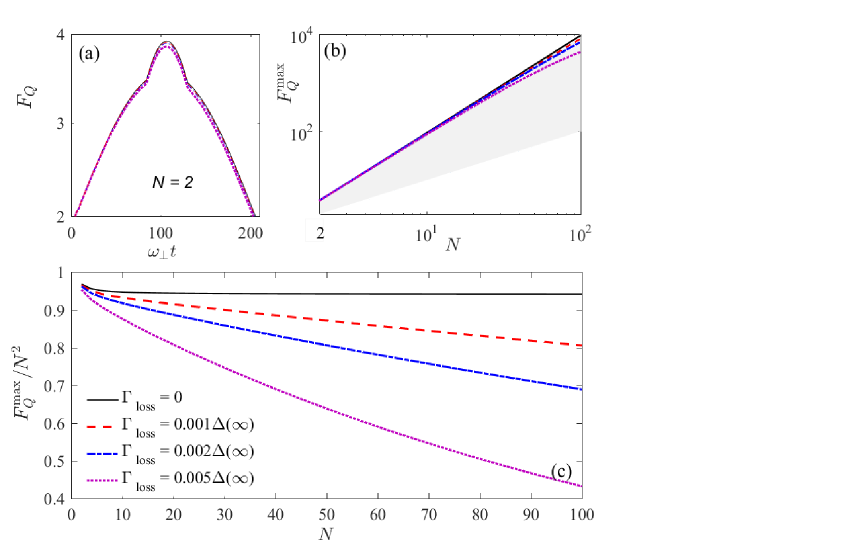
Figures 5(b) and (c) illustrate the QFI with respect to atom number for different values of loss parameters. As shown in Fig. 5(b), under the values of we considered, we can obtain near-Heisenberg scaling. Figures 5(c) plots the rates of the Heisenberg limit with respect to atom number for different values of loss parameters . It indicates that for not too large , we can obtain the Heisenberg scaling only with a prefactor. We can also see, when increasing the loss rate the values of degrades with the increasing of number of atoms , since the collective dissipate rare depends on . Fortunately, for the low temperature limit we considered the values of is not too large, hence we can still obtain the robust sub-shot-noise-limited phase sensitivity.
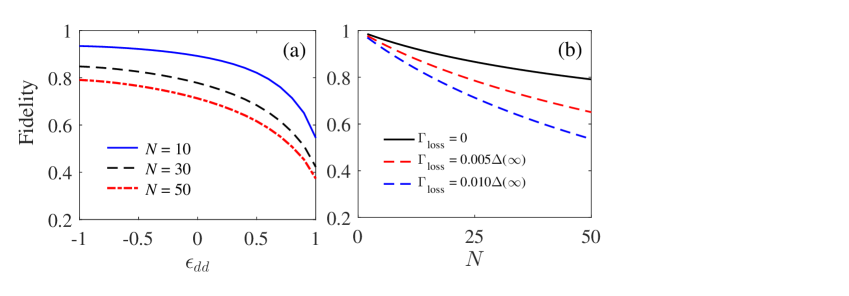
To demonstrate the near Heisenberg-limited sensitivity with the ENGSs realized by our model, we calculate the fidelity between the optimal ENGSs and spin cat states Momer , which are the maximal entangled states and have the Heisenberg-limited sensitivity for metrology. It is given by
| (34) |
where is the CSS. With the definition of fidelity, we have
| (35) |
where .
Form Fig. 6, we can find that the fidelity depends on both the and particle number . The maximal values occurs at . Because of the dissipative rate , the fidelity decrease with the increase of . As shown in Fig. 6(a), when we get , and for , and . And the effect of on fidelity also is shown in Fig. 6(b).
VI conclusion
In summary, we have realized the SSSs and ENGSs by immersing atoms in a thermally equilibrated quasi-1D dipolar BEC reservoir. It has demonstrated that the repulsive-dipolar-interaction reservoir can induce better SS and entanglement. We have shown that owing to the dephasing noise, even in the regimes without SS the ENGSs can successively undergo highly metastable entangled states and entanglement suddenly increase. To explain the highly sensitivity for metrology, we calculated the fidelity between the optimal ENGSs and spin cat states, and found that the optimal ENGS is similar to the spin cat state. It has confirmed that by the use of ENGSs for metrology, the phase estimation sensitivity can surpass that by SS and even approach to Heisenberg limit for neglectable atom loss rates. The effect of the atom loss rate as a free parameter has also been considered.
Finally, we give two remarks on the above obtained results: First, these results we have obtained in this paper are based on the negligible spatial evolution of the immersed condensate wave functions. Usually this assumption is enough to capture the basic processes and physics, and detailed consideration of the impact of spatial dynamics can be investigated by adopting the multi-configurational time-dependent Hartree for bosons method stre2006 . Second, the scheme we proposed in this work can also suit the case that the system atoms are weak or no interaction two-level impurity atoms which are not condensate.
Acknowledgements.
This work was supported by the NSFC under Grant No. 11547159. G.R.J. acknowledges support from the Major Research Plan of the NSFC (Grant No. 91636108).Appendix A Derivation of Eq. (7)
Here, we present a detailed derivation of the Fourier transform of the effective 1D interaction potential. It can be obtained by integrating out the and variables as
| (36) | |||||
When assuming the dipole moments lie on the plane forming an angle to axis, i.e.,
| (37) |
Then, we have
| (38) | |||||
where with and . Clearly, the effective 1D dipolar interaction vanishes at the magical angle , and it is attractive (repulsive) for . In the main text, we have dropped the tilde on and , and will only consider the values of .
Appendix B Time evolution operator
The time evolution operator can be obtained by using Magnus expansion
| (39) |
Note that only the below first two terms of the expansion are non-zero
| (40) | |||||
| (41) | |||||
with the amplitudes , since which commutes with the high order terms. It is worth to point out that the commutator of the interaction Hamiltonian at two different times is an operator but not a number as considering in the single bit case, which can induce the nonlinear interaction; the noise-induced nonlinear interaction strengthen can recast as
| (42) | |||||
where we have used the relation . Then,
| (43) | |||||
where and is the global phase and will be dropped.
Appendix C Spin squeezing with
In this Appendix, we present a detailed of SS with . To this end, we assume, without loss of generality, that , where and are polar and azimuthal angles, respectively. We then define two mutually perpendicular unit vectors and . Clearly, both and are perpendicular to such that form a right-hand frame. Now, the minimal fluctuation of a spin component perpendicular to the mean spin is
| (44) |
and the mean spin is
| (45) |
where
with
Appendix D Matrix elements of for
The matrix elements for the symmetric matrix in plane are
| (47) |
with
| (48) |
| (49) |
References
- (1) C. M. Caves, Phys. Rev. D 23, 1693 (1981).
- (2) B. Yurke, S. L. McCall, and J. R. Klauder, Phys. Rev. A 33, 4033 (1986).
- (3) M. J. Holland and K. Burnett, Phys. Rev. Lett. 71, 1355 (1993).
- (4) U. Dorner, R. Demkowicz-Dobrzanski, B. J. Smith, J. S. Lundeen, W. Wasilewski, K. Banaszek, and I. A. Walmsley, Phys. Rev. Lett. 102, 040403 (2009).
- (5) V. Giovannetti, S. Lloyd, and L. Maccone, Nat. Photon. 5, 222 (2011).
- (6) B. C. Sanders and G. J. Milburn, Phys. Rev. Lett. 75, 2944 (1995).
- (7) J. Ma, X. Wang, C. P. Sun, and F. Nori, Phys. Rep. 509, 89 (2011).
- (8) J. Ma, Y. X. Huang, X. Wang, and C. P. Sun, Phys. Rev. A 84, 022302 (2011).
- (9) P. C. Humphreys, M. Barbieri, A. Datta, and I. A. Walmsley, Phys. Rev. Lett. 111, 070403 (2013).
- (10) J. P. Dowling, Contemp. Phys. 49, 125 (2008).
- (11) A. I. Lvovsky, B. C. Sanders, and W. Tittel, Nat. Photon. 3, 706 (2009)
- (12) M. Kitagawa and M. Ueda, Phys. Rev. A 47, 5138 (1993).
- (13) D. J. Wineland, J. J. Bollinger, W. M. Itano, D. J. Heinzen, Phys. Rev. A 50, 67 (1994).
- (14) K. Mømer and A. Søensen, Phys. Rev. Lett. 82, 1835 (1999).
- (15) A. Sørensen, L-M. Duan, J. I. Cirac and P. Zoller, Nature 409, 4 (2001).
- (16) U. V. Poulsen and K. Mølmer, Phys. Rev. A 64, 013616 (2001).
- (17) G. R. Jin, Y. C. Liu and W. M. Liu, New J. Phys. 11, 073049 (2009).
- (18) G. R. Jin, Y. An, T. Yan, and Z. S. Lu, Phys. Rev. A 82, 063622 (2010).
- (19) O. Guehne and G. Tóth, Phys. Rep. 474, 1 (2009).
- (20) X. Wang and B. C. Sanders, Phys. Rev. A 68, 012101 (2003).
- (21) Y. C. Liu, Z. F. Xu, G. R. Jin, and L. You, Phys. Rev. Lett. 107, 013601 (2011).
- (22) H. Strobel, W. Muessel, D. Linnemann, T. Zibold, D. B. Hume, L. Pezzé, A. Smerzi and M. K. Oberthaler, science 345, 424 (2014).
- (23) T. Macrì, A. Smerzi, and L. Pezzé, Phys. Rev. A 94, 010102 ( 2016).
- (24) S. D. Bennett, N.Y. Yao, J. Otterbach, P. Zoller, P. Rabl, and M. D. Lukin, Phys. Rev. Lett. 110, 156402 (2013).
- (25) P. Bouyer and M. A. Kasevich, Phys. Rev. A 56, R1083 (1997).
- (26) M. A. Kasevich, Science, 298, 1363 (2002).
- (27) C. Gross, T. Zibold, E. Nicklas, J. Estève and M. K. Oberthaler, Nature (London) 464, 1165 (2010).
- (28) M. F. Riedel, P. Böhi, Y. Li, T. W. Hansch, A. Sinatra and P. Treutlein, Nature (London) 464, 1170 (2010).
- (29) S. Palzer, C. Zipkes, C. Sias, and M. Köhl, Phys. Rev. Lett. 103, 150601 (2009).
- (30) M. A. Cirone, G. De. Chiara, G. M. Palma, and A. Recati, New J. Phys. 11, 103055 (2009).
- (31) S. Will, T. Best, S. Braun, U. Schneider, and I. Bloch, Phys. Rev. Lett. 106, 115305 (2011).
- (32) N. Spethmann, F. Kindermann, S. John, C. Weber, D. Meschede, and A. Widera, Phys. Rev. Lett. 109, 235301 (2012).
- (33) R. Scelle, T. Rentrop, A. Trautmann, T. Schuster, and M. K. Oberthaler, Phys. Rev. Lett. 111, 070401 (2013).
- (34) C. Zipkes, S. Palzer, C. Sias, and M. Köhl, Nature (London) 464, 388 (2010).
- (35) S. Schmid, A. Harter, and J. H. Denschlag, Phys. Rev. Lett. 105, 133202 (2010).
- (36) J. B. Balewski, A. T. Krupp, A. Gaj, D. Peter, H. P. Büchler, R. Löw, S. Hofferberth, and T. Pfau, Nature (London) 502, 664 (2013).
- (37) A. Recati, P. O. Fedichev, W. Zwerger, J. von Delft, and P. Zoller, Phys. Rev. Lett. 94, 040404 (2005).
- (38) H. T. Ng and S. Bose, Phys. Rev. A 78, 023610 (2008).
- (39) N. Bar-Gill, D. D. Bhaktavatsala Rao, and G. Kurizki, Phys. Rev. Lett. 107, 010404 (2011).
- (40) M. Bruderer and D. Jaksch, New J. Phys. 8, 87 (2006).
- (41) S. Yi and L. You, Phys. Rev. A 61, 041604(R) (2000); 63, 053607 (2001).
- (42) K. Goral, L. Santos, and M. Lewenstein, Phys. Rev. Lett. 88, 170406 (2002)
- (43) S. Yi, L. You, and H. Pu, Phys. Rev. Lett. 93, 040403 (2004).
- (44) S. Yi, T. Li, and C. P. Sun, Phys. Rev. Lett. 98, 260405 (2007).
- (45) H.-Y. Lu and S. Yi, Sci China-Phys Mech Astron 55, 1535 (2012).
- (46) M. Lu, N. Q. Burdick, S. H. Youn, and B. L. Lev, Phys. Rev. Lett. 107, 190401 (2011).
- (47) K. Aikawa, A. Frisch, M. Mark, S. Baier, A. Rietzler, R. Grimm, and F. Ferlaino, Phys. Rev. Lett. 108, 210401 (2012).
- (48) S. Giovanazzi, A. Görlitz, and T. Pfau, Phys. Rev. Lett. 89, 130401 (2002).
- (49) T. Lahaye, C. Menotti, L. Santos, M. Lewenstein, and T. Pfau, Rep. Prog. Phys. 72, 126401 (2009).
- (50) A. Griesmaier, J. Stuhler, T. Koch, M. Fattori, T. Pfau, and S. Giovanazzi, Phys. Rev. Lett. 97, 250402 (2006).
- (51) J. B. Yuan, H.-J Xing, L.-M. Kuang, and S. Yi, Phys Rev A 95, 033610 (2017).
- (52) K. Pawlowski, K. Rzazewski, Phys Rev A 81, 013620 (2010).
- (53) Y. Hao and Q. Gu, Phys Rev A 83, 043620 (2011).
- (54) D. Spehner, K. Pawlowski, G. Ferrini, and A. Minguzzi, Eur. Phys. J. B 87, 156 (2014).
- (55) J. Huang, X. Qin, H. Zhong, Y. Ke and C. Lee, Sci Rep. 5, 17894 (2015).
- (56) F. Dalfovo, S. Giorgini, L. P. Pitaevskii, and S. Stringari, Rev. Mod. Phys. 71, 463 (1999).
- (57) H. P. Breuer and F. Petruccione, The Theory of Open Quantum Systems (Oxford University Press, Oxford, 2007).
- (58) A. I. Streltsov, O. E. Alon, L. S. Cederbaum, Phys Rev A 73, 063626 (2006); O. E. Alon, A. I. Streltsov, L. S. Cederbaum, Phys Rev A 77, 033613 (2008).