smAdditional References
Nearest-Neighbor Mixture Models for Non-Gaussian Spatial Processes
Abstract
We develop a class of nearest-neighbor mixture models that provide direct, computationally efficient, probabilistic modeling for non-Gaussian geospatial data. The class is defined over a directed acyclic graph, which implies conditional independence in representing a multivariate distribution through factorization into a product of univariate conditionals, and is extended to a full spatial process. We model each conditional as a mixture of spatially varying transition kernels, with locally adaptive weights, for each one of a given number of nearest neighbors. The modeling framework emphasizes the description of non-Gaussian dependence at the data level, in contrast with approaches that introduce a spatial process for transformed data, or for functionals of the data probability distribution. Thus, it facilitates efficient, full simulation-based inference. We study model construction and properties analytically through specification of bivariate distributions that define the local transition kernels, providing a general strategy for modeling general types of non-Gaussian data. Regarding computation, the framework lays out a new approach to handling spatial data sets, leveraging a mixture model structure to avoid computational issues that arise from large matrix operations. We illustrate the methodology using synthetic data examples and an analysis of Mediterranean Sea surface temperature observations.
Keywords: Bayesian hierarchical models; Copulas; Spatial generalized linear mixed model; Spatial statistics; Vecchia approximations
1 Introduction
Gaussian processes have been widely used as an underlying structure in model-based analysis of irregularly located spatial data in order to capture short range variability. The fruitfulness of these spatial models owes to the simple characterization of the Gaussian process by a mean and a covariance function, and the optimal prediction it provides that justifies kriging. However, the assumption of Gaussianity is restrictive in many fields where the data exhibits non-Gaussian features, for example, vegetation abundance (Eskelson et al., 2011), precipitation data (Sun et al., 2015), temperature data (North et al., 2011), and wind speed data (Bevilacqua et al., 2020). This article aims at developing a flexible class of geostatistical models that is customizable to general non-Gaussian distributions, with particular focus on continuous data.
Several approaches have been developed for non-Gaussian geostatistical modeling. A straightforward approach consists of fitting a Gaussian process after transformation of the original data. Possible transformations include Box-Cox (De Oliveira et al., 1997), power (Allcroft and Glasbey, 2003), square-root (Johns et al., 2003), and Tukey g-and-h (Xu and Genton, 2017) transforms, to name a few. An alternative approach is to represent a non-Gaussian distribution as a location-scale mixture of Gaussian distributions. This yields Gaussian process extensions that are able to capture skewness and long tails (Kim and Mallick, 2004; Palacios and Steel, 2006; Zhang and El-Shaarawi, 2010; Mahmoudian, 2017; Morris et al., 2017; Zareifard et al., 2018; Bevilacqua et al., 2021). Beyond methods based on continuous mixtures of Gaussian distributions, Bayesian nonparametric methods have been explored for geostatistical data modeling, starting with the approach in Gelfand et al. (2005) which extends the Dirichlet process (Ferguson, 1973) to a prior model for random spatial surfaces. We refer to Müller et al. (2018) for a review. From a different perspective, Bolin (2014) formulates stochastic partial differential equations driven by non-Gaussian noise, resulting in a class of non-Gaussian Matérn fields.
An alternative popular approach involves a hierarchical model structure that assumes conditionally independent non-Gaussian marginals, combined with a latent spatial process that is associated with some functional or link function of the first-stage marginals. Hereafter, we refer to these models as hierarchical first-stage non-Gaussian models. If the latent process is linked through a function of some parameter(s) of the first-stage marginal which belongs to the exponential dispersion family, the approach is known as the spatial generalized linear mixed model and its extensions (Diggle et al., 1998). Non-Gaussian spatial models that build from copulas (Joe, 2014) can also be classified into this category. Copula models assume pre-specified families of marginals for observations, with a multivariate distribution underlying the copula for a vector of latent variables that are probability integral transformations of the observations (Danaher and Smith, 2011). Spatial copula models replace the multivariate distribution with one that corresponds to a spatial process, thus introducing spatial dependence (Bárdossy, 2006; Ghosh and Mallick, 2011; Krupskii et al., 2018; Beck et al., 2020).
The non-Gaussian modeling framework proposed in this article is distinctly different from the previously mentioned approaches. Our methodology builds on the class of nearest-neighbor processes obtained by extending a joint density for a reference set of locations to the entire spatial domain. The original joint density is factorized into a product of conditionals with respect to a sparse directed acyclic graph (DAG). Deriving each conditional from a Gaussian process results in the nearest-neighbor Gaussian process (Datta et al., 2016a). Models defined over DAGs have received substantial attention; see, e.g., Datta et al. (2016b); Finley et al. (2019); Peruzzi et al. (2020); Peruzzi and Dunson (2022). The class of DAG-based models originates from the Vecchia approximation framework (Vecchia, 1988). Katzfuss and Guinness (2021) provide further generalization. Considerably less attention, however, has been devoted to defining models over a sparse DAG with non-Gaussian distributions for the conditionals of the joint density. This is in general a difficult problem, as each conditional involves, say, a -dimensional conditioning set, which requires a coherent model for a -dimensional non-Gaussian distribution, with potentially large. In this article, we take on the challenging task of developing a computationally efficient, interpretable framework that provides generality for modeling different types of non-Gaussian data and flexibility for complex spatial dependence.
We overcome the aforementioned challenge by modeling each conditional of the joint density as a weighted combination of spatially varying transition kernels, each of which depends on a specific neighbor. This approach produces multivariate non-Gaussian distributions by specification of the bivariate distributions that define the local transition kernels. Thus, it provides generality for modeling different non-Gaussian behaviors, since, relative to the multivariate analogue, constructing bivariate distributions is substantially easier, for instance, using bivariate copulas. Moreover, such a model structure offers the convenience of quantifying multivariate dependence through the collection of bivariate distributions. As an illustration, we study tail dependence properties under appropriate families of bivariate distributions, and provide results that guide modeling choices. The modeling framework achieves flexibility by letting both the weights and transition kernels be spatially dependent, inducing sufficient local dependence to describe a wide range of spatial variability. We refer to the resulting geospatial process as the nearest-neighbor mixture process (NNMP).
An important feature of the model structure is that it facilitates the study of conditions for constructing NNMPs with pre-specified families of marginal distributions. Such conditions are easily implemented without parameter constraints, thus resulting in a general modeling tool to describe spatial data distributions that are skewed, heavy-tailed, positive-valued, or have bounded support, as illustrated through several examples in Section 4 and in the supplementary material. The NNMP framework emphasizes direct modeling by introducing spatial dependence at the data level. It avoids the use of transformations that may distort the Gaussian process properties (Wallin and Bolin, 2015). It is fundamentally different from the class of hierarchical first-stage non-Gaussian models that introduce spatial dependence through functionals of the data probability distribution, such as the transformed mean. Regarding computation, NNMP models do not require estimation of potentially large vectors of spatially correlated latent variables, something unavoidable with hierarchical first-stage non-Gaussian models. In fact, approaches for such models typically resort to approximate inference, either directly or combined with a scalable model (Zilber and Katzfuss, 2021). Estimation of NNMPs is analogous to that of a finite mixture model, thus avoiding the need to perform costly matrix operations for large data sets, and allowing for computationally efficient, full simulation-based inference. Overall, the NNMP framework offers a flexible class of models that is able to describe complex spatial dependence, coupled with an efficient computational approach, leveraged from the mixture structure of the model.
The rest of the article is organized as follows. In Section 2, we formulate the NNMP framework and study model properties. Specific examples of NNMP models illustrate different components of the methodology. Section 3 develops the general approach to Bayesian estimation and prediction under NNMP models. In Section 4, we demonstrate different NNMP models with a synthetic data example and with the analysis of Mediterranean Sea surface temperature data, respectively. Finally, Section 5 concludes with a summary and discussion of future work.
2 Nearest-Neighbor Mixture Processes for Spatial Data
2.1 Modeling Framework
Consider a univariate spatial process , where , for . Let be a finite collection of locations in , referred to as the reference set. We write the joint density of the random vector as . If we regard the conditioning set of as the parents of , the joint density is a factorization according to a DAG whose vertices are . We obtain a sparse DAG by reducing the conditioning set of to a smaller subset, denoted as , with . We refer to as the neighbor set for , having at most elements with . The resulting density for the sparse DAG is
| (1) |
which is a proper density (Lauritzen, 1996). Choosing the neighbor sets creates different sparse DAGs. There are different ways to select members from for ; see, e.g., Vecchia (1988), Stein et al. (2004), and Gramacy and Apley (2015). Our selection is based on the geostatistical distance between and . The selected locations are placed in ascending order according to the distance, denoted as , where . We note that the development of the proposed framework holds true for any choice of the neighbor sets.
Constructing a nearest-neighbor process involves specification of the conditional densities in (1), and extension to an arbitrary finite set in that is not overlapping with . We approach the problem of constructing a nearest-neighbor non-Gaussian process following this idea. A notable difference, however, from the nearest-neighbor Gaussian process approach in Datta et al. (2016a) is that we do not posit a parent process for when deriving . Datta et al. (2016a) assume a Gaussian process for , and use it to model the conditional densities . Similar ideas underlie the Vecchia approximation framework which considers (1) as an approximation for the density of a Gaussian process realization. We instead utilize the structure in (1) to develop nearest-neighbor models for non-Gaussian spatial processes. To this end, we define the conditional density in the product in (1) as
| (2) |
where is the th component of the mixture density , and the weights satisfy , for all , and , for every . In a sparse DAG, nearest neighbors in set are nodes that have directed edges pointing to . Thus, it is appealing to consider a high-order Markov model in which temporal lags have a similar notion of direction. Our approach to formulate (2) is motivated from a class of mixture transition distribution models (Le et al., 1996), which consists of a mixture of first-order transition densities with a vector of common weights. A key feature of the formulation in (2) is the decomposition of a non-Gaussian conditional density, with a potentially large conditioning set, into a weighted sum of local conditional densities. This provides flexible, parsimonious modeling of through specifying bivariate distributions that define the local conditionals . We provide further discussion on this feature for model construction and relevant properties in the following sections.
Spatial dependence characterized by (2) is twofold. First, each component is associated with spatially varying parameters indexed at , defined by a probability model or a link function. Secondly, the weights are spatially varying. As each component density depends on a specific neighbor, the weights indicate the contribution of each neighbor of . Besides, the weights adapt to the change of locations. For two different in , the relative locations of the nearest neighbors to are different from that of to . If all elements of are very close to , then values of should be quite even. On the other hand, if, for , only a subset of its neighbors in are close to , then the weights corresponding to this subset should receive larger values. We remark that in general, probability models or link functions for the spatially varying parameters should be considered case by case, given different specifications on the components . Details of the construction for the component densities and the weights are deferred to later sections.
We obtain the NNMP, a legitimate spatial process, by extending (2) to an arbitrary set of non-reference locations where . In particular, we define the conditional density of given as
| (3) |
where the specification on and for all and all is analogous to that for (2), except that are the first locations in that are closest to in terms of geostatistical distance. Building the construction of the neighbor sets on the reference set ensures that is a proper density.
Given (2) and (3), we can obtain the joint density of a realization over any finite set of locations . When , the joint density is directly available as the appropriate marginal of . Otherwise, we have , where . If is empty, is simply . In general, the joint density of an NNMP is intractable. However, since both and are products of mixtures, we can recognize that is a finite mixture, which suggests flexibility of the model to capture complex non-Gaussian dependence over the domain . Moreover, we show in Section 2.3 that for some NNMPs, the joint density has a closed-form expression. In the subsequent development of model properties, we will use the conditional density
| (4) |
to characterize an NNMP, where contains the first locations that are closest to , selected from locations in . These locations in are placed in ascending order according to distance, denoted as .
Before closing this section, we note that spatial locations are not naturally ordered. Given a distance function, a different ordering on the locations results in different neighbor sets. Therefore, a different sparse DAG with density is created accordingly for model inference. For the NNMP models illustrated in the data examples, we found through simulation experiments that there were no discernible differences between the inferences based on , given two different orderings. This observation is coherent with that from the literature that considers nearest-neighbor likelihood approximations. Since the approximation of to depends on the information borrowed from the neighbors, as outlined in Datta et al. (2016a), the effectiveness is determined by the size of rather than the ordering. A further remark is that, the ordering of the reference set is typically reserved for observed data. Thus, the ordering effect lies only in the model estimation based on (2) with realization . Spatial prediction typically rests on locations outside using (3), where the ordering effect disappears.
2.2 NNMPs with Stationary Marginal Distributions
We develop a sufficient condition to construct NNMPs with general stationary marginal distributions. The key feature of this result is that the condition relies on the bivariate distributions that define the first order transition kernels in (4) without the need to impose restrictions on the parameter space. The supplementary material includes the proof of Proposition 1, as well as of Propositions 2, 3 and 4, and of Corollary 1, formulated later in Sections 2.3 and 2.4.
Proposition 1.
Consider an NNMP for which the component density is specified by the conditional density of given , where the random vector follows a bivariate distribution with marginal densities and , for . The NNMP has stationary marginal density if it satisfies the invariant condition: , , and for every , , for all and for all .
This result builds from the one in Zheng et al. (2022) where mixture transition distribution models with stationary marginal distributions were constructed. It applies regardless of being a continuous, discrete or mixed random variable, thus allowing for a wide range of non-Gaussian marginal distributions and a general functional form, either linear or non-linear, for the expectation with respect to the conditional density in (4).
As previously discussed, the mixture model formulation for the conditional density in (4) induces a finite mixture for the NNMP finite-dimensional distributions. On the other hand, due to the mixture form, an explicit expression for the covariance function is difficult to derive. A recursive equation can be obtained for a class of NNMP models for which the conditional expectation with respect to is linear, that is, for some , and for all . Suppose the NNMP has a stationary marginal distribution with finite first and second moments. Without loss of generality, we assume the first moment is zero. Then the covariance over any two locations is
| (5) |
where , , , and without loss of generality, we assume . The covariance in (5) implies that, even though the NNMP has a stationary marginal distribution, it is second-order non-stationary.
2.3 Construction of NNMP Models
The spatially varying conditional densities in (4) correspond to a sequence of bivariate distributions indexed at , namely, the distributions of , for . To balance model flexibility and scalability, we build spatially varying distributions by considering the distribution of random vector , for , and extending some of its parameters to be spatially varying, that is, indexed in . To this end, we use a probability model or a link function. We refer to the random vectors as the set of base random vectors. With a careful choice of the model/function for the spatially varying parameter(s), this construction method reduces significantly the dimension of the parameter space, while preserving the capability of the NNMP model structure to capture spatial dependence.
We illustrate the method with several examples below, starting with a bivariate Gaussian distribution and its continuous mixtures for real-valued data, followed by a general strategy using bivariate copulas that can model data with general support. Before proceeding to the examples, we emphasize that our method allows for general bivariate distributions. One can also consider using a pair of compatible conditionals to specify bivariate distributions (Arnold et al., 1999), for instance, a pair of Lomax conditionals. This is illustrated in Example 4 in Section 2.4.
Example 1.
Gaussian and continuous mixture of Gaussian NNMP models.
For , take to be a bivariate Gaussian random vector with mean and covariance matrix , where is the two-dimensional column vector of ones, resulting in a Gaussian conditional density . If we extend the correlation parameter to be spatially varying, , for a correlation function , we obtain the spatially varying conditional density,
| (6) |
This NNMP is referred to as the Gaussian NNMP. If we take , and set and , for all , the resulting model satisfies the invariant condition of Proposition 1 with stationary marginal given by the distribution. The finite-dimensional distribution of the Gaussian NNMP is characterized by the following proposition.
Proposition 2.
Consider the Gaussian NNMP in (6) with and , for all . If , the Gaussian NNMP has the stationary marginal distribution, and its finite-dimensional distributions are mixtures of multivariate Gaussian distributions.
We refer to the model in Proposition 2 as the stationary Gaussian NNMP. Based on the Gaussian NNMP, various NNMP models with different families for can be constructed by exploiting location-scale mixtures of Gaussian distributions. We illustrate the approach with the skew-Gaussian NNMP model. Denote by the Gaussian distribution with mean and variance , truncated at the interval . Building from the Gaussian NNMP, we start with a conditional bivariate Gaussian distribution for , given , where is replaced with . Marginalizing out yields the bivariate skew-Gaussian distribution for (Azzalini, 2013). Extending again to , for all , we can express the conditional density for the skew-Gaussian NNMP model as where we have: ; ; ; and . Setting , , and , for all , we obtain the stationary skew-Gaussian NNMP model, with skew-Gaussian marginal , denoted as .
The skew-Gaussian NNMP model is an example of a location mixture of Gaussian distributions. Scale mixtures can also be considered to obtain, for example, the Student-t model. In that case, we replace the covariance matrix with , taking as a random variable with an appropriate inverse-gamma distribution. Important families that admit a location and/or scale mixture of Gaussians representation include the skew-t, Laplace, and asymmetric Laplace distributions. Using a similar approach to the one for the skew-Gaussian NNMP example, we can construct the corresponding NNMP models.
Example 2.
Copula NNMP models.
A copula function is a function such that, for any multivariate distribution , there exists a copula for which , where is the marginal distribution function of , (Sklar, 1959). If is continuous for all , is unique. A copula enables us to separate the modeling of the marginal distributions from the dependence. Thus, the invariant condition in Proposition 1 can be attained by specifying the stationary distribution as the marginal distribution of for all . The copula parameter that determines the dependence of can be modeled as spatially varying to create a sequence of spatially dependent bivariate vectors . Here, we focus on continuous distributions, although this strategy can be applied for any family of distributions for . We consider bivariate copulas with a single copula parameter, and illustrate next the construction of a copula NNMP given a stationary marginal density .
For the bivariate distribution of each with marginals and , we consider a copula with parameter , for . We obtain a spatially varying copula for by extending to . The joint density of is given by , where is the copula density of , and and are the marginal densities of and , respectively. Given a pre-specified stationary marginal , we replace both and with , for every and for all . We then obtain the conditional density
| (7) |
that characterizes the stationary copula NNMP.
Under the copula framework, one strategy to specify the spatially varying parameter is through the Kendall’s coefficient. The Kendall’s , taking values in , is a bivariate concordance measure with properties useful for non-Gaussian modeling. In particular, its existence does not require finite second moment and it is invariant under strictly increasing transformations. If is continuous with a copula , its Kendall’s is . Taking as the range of , we can construct a composition function for some link function and kernel function , where is the parameter space associated with . The kernel should be specified with caution; must satisfy axioms in the definition of a bivariate concordance measure (Joe 2014, Section 2.12). We illustrate the strategy with the following example.
Example 3.
The bivariate Gumbel copula is an asymmetric copula useful for modeling dependence when the marginals are positive and heavy-tailed. The spatial Gumbel copula can be defined as , where and perfect dependence is obtained if . The Kendall’s is , taking values in . We define , an isotropic correlation function. Let . Then, the function . Thus, the parameter is given by , and as .
After we define a spatially varying copula, we obtain a family of copula NNMPs by choosing a desired family of marginal distributions. Section 4.1 illustrates Gaussian and Gumbel copula NNMP models with gamma marginals, and the supplementary material provides an additional example of a Gaussian copula NNMP with beta marginals.
Copula NNMP models offer avenues to capture complex dependence using general bivariate copulas. Traditional spatial copula models specify the finite dimensional distributions of the underlying spatial process with a multivariate copula. However, multivariate copulas need to be used with careful consideration in a spatial setting. For example, it is common to assume that spatial processes exhibit stronger dependence at smaller distances. Thus, copulas such as the multivariate Archimedean copula that induce an exchangeable dependence structure are inappropriate. Though spatial vine copula models (Gräler, 2014) can resolve this restriction, their model structure and computation are substantially more complicated than copula NNMP models.
2.4 Mixture Component Specification and Tail Dependence
A benefit of building NNMPs from a set of base random vectors is that specification of the multivariate dependence of given its neighbors is determined mainly by that of the base random vectors. In this section, we illustrate this attractive property of the model with the establishment of lower bounds for two measures used to assess strength of tail dependence.
The main assumption is that the base random vector has stochastically increasing positive dependence. is said to be stochastically increasing in , if increases as increases. The definition can be extended to a multivariate random vector . is said to be stochastically increasing in if , for all and in the support of , where , for . The conditional density in (4) implies that
Therefore, is stochastically increasing in if is stochastically increasing in with respect to for all . If the sequence is built from the vector , then the set of base random vectors determines the stochastically increasing positive dependence of given its neighbors.
For a bivariate random vector , the upper and lower tail dependence coefficients, denoted as and , respectively, are and . When , we say and have upper tail dependence. When , and are said to be asymptotically independent in the upper tail. Lower tail dependence and asymptotically independence in the lower tail are similarly defined using . Let be the marginal distribution function of . Analogously, we can define the upper and lower tail dependence coefficients for given its nearest neighbors,
The following proposition provides lower bounds for the tail dependence coefficients.
Proposition 3.
Consider an NNMP for which the component density is specified by the conditional density of given , where the random vector follows a bivariate distribution with marginal distribution functions and , for . The spatial dependence of random vector is built from the base vector , which has a bivariate distribution such that is stochastically increasing in , for . Then, for every , the lower bound for the upper tail dependence coefficient is , and the lower bound for the lower tail dependence coefficient is .
Proposition 3 establishes that the lower and upper tail dependence coefficients are bounded below by a convex combination of, respectively, the limits of the conditional distribution functions and the conditional survival functions. These are fully determined by the dependence structure of the bivariate distribution for . The result is best illustrated with an example.
Example 4.
Consider a Lomax NNMP for which the bivariate distributions of the base random vectors correspond to a bivariate Lomax distribution (Arnold et al., 1999), resulting in conditional density, , where denotes the Lomax density, a shifted version of the Pareto Type I density. A small value of indicates a heavy tail. The component conditional survival function of the Lomax NNMP, expressed in terms of the quantile , is which converges to as . Therefore, the lower bound for is . As for all , the lower bound for tends to one, and hence tends to one, since . As for all , the lower bound tends to zero.
Proposition 3 holds for the general framework. If the distribution of with has first order partial derivatives and exchangeable dependence, namely and have the same joint distribution, the lower bounds of the tail dependence coefficients depend on the component tail dependence coefficients. The result is summarized in the following corollary.
Corollary 1.
Suppose that the base random vector in Proposition 3 is exchangeable, and its bivariate distribution with marginals has first order partial derivatives, for all . Then the upper and lower tail dependence coefficients and are bounded below by and , where and are the tail dependence coefficients with respect to .
Under Corollary 1, if the bivariate distribution of is symmetric, for instance, an elliptically symmetric distribution, the upper and lower tail dependence coefficients coincide, and can simply be denoted as . Then, we have that , where is the tail dependence coefficient with respect to .
Tail dependence can also be quantified using the boundary of the conditional distribution function, as proposed in Hua and Joe (2014) for a bivariate random vector. In particular, the upper tail dependence of is said to have some strength if is positive at . Likewise, a non-zero at indicates some strength of dependence in the lower tails. The functions and are referred to as the boundary conditional distribution functions.
We use for simpler notation for the conditional distribution function of , . Then and are the boundary conditional distribution functions for the NNMP model. The upper tail dependence is said to be i) strongest if equals for and has a mass of 1 at ; ii) intermediate if has positive but not unit mass at ; iii) weakest if has no mass at . The strength of lower tail dependence is defined likewise using . The following result gives lower bounds for the boundary conditional distribution functions.
Proposition 4.
Consider an NNMP for which the component density is specified by the conditional density of given . The spatial dependence of random vector is built from the base vector , which has a bivariate distribution such that is stochastically increasing in , for . Let and be the lower and upper tail dependence coefficients corresponding to . If for a given , there exists for some , then the conditional distribution function has strictly positive mass at with . Similarly, if for a given , there exists for some , then the conditional distribution function has strictly positive mass at with .
Proposition 4 complements Proposition 3 to assess strength of tail dependence. It readily applies for bivariate distributions, especially for copulas which yield explicit expressions for the tail dependence coefficients. In particular, the spatially varying Gumbel copula in Example 3 has upper tail dependence coefficient for , so the tail dependence of a Gumbel copula NNMP model has some strength if for some . In fact, applying the result in Hua and Joe (2014), with a Gumbel copula, degenerates at , implying strongest tail dependence.
3 Bayesian Hierarchical Model and Inference
3.1 Hierarchical Model Formulation
We introduce the general approach for NNMP Bayesian implementation, treating the observed spatial responses as an NNMP realization. The inferential framework can be easily extended to incorporate model components that may be needed in practical settings, such as covariates and additional error terms. We illustrate the extensions with the real data analysis in Section 4.2 and in the supplementary material, and provide further discussion in Section 5.
Our approach for inference is based on a likelihood conditional on the first elements of the realization over the reference set . Following a commonly used approach for mixture models fitting, we use data augmentation to facilitate inference. For each , , we introduce a configuration variable , taking values in , such that , where , and if and otherwise. Conditional on the configuration variables and the vector , the augmented model is
| (8) |
where collects the parameters of the densities .
A key component of the Bayesian model formulation is the prior model for the weights. Weights are allowed to vary in space, adjusting to the neighbor structure of different reference locations. We describe the construction for weights corresponding to a point in the reference set. For non-reference points, weights are defined analogously. Consider a collection of spatially dependent distribution functions supported on . For each , the weights are defined as the increments of with cutoff points . More specifically,
| (9) |
where denotes the indicator function for set . The cutoff points are such that, for , , where is a bounded kernel function with parameters . The kernel and its associated parameters affect the smoothness of the resulting random field. We take as a logit Gaussian distribution, denoted as , such that the corresponding Gaussian distribution has mean and variance . The spatial dependence across the weights is introduced through the mean , where . Given the cutoff points and , a small value of favors large weights for the near neighbors of . A simpler version of the model in (9) is obtained by letting be the uniform distribution on . Then the weights become . We notice that Cadonna et al. (2019) use a set of fixed, uniform cutoff points on , i.e., , for spectral density estimation, with a collection of logit Gaussian distributions indexed by frequency.
The full Bayesian model is completed with prior specification for parameters , and . The priors for and depend on the choices of the densities and the cutoff point kernel , respectively. For parameters and , we specify and priors, respectively, where denotes the inverse gamma distribution.
Finally, we note that an NNMP model requires selection of the neighborhood size . This can be done using standard model comparison metrics, scoring rules, or information criteria; for example, Datta et al. (2016a) used root mean square predictive error and Guinness (2018) used Kullback–Leibler divergence. In general, a larger increases computational cost. Datta et al. (2016a) conclude that a moderate value typically suffices for the nearest-neighbor Gaussian process models. Peruzzi et al. (2020) point out that a smaller corresponds to a larger Kullback–Leibler divergence of from , regardless of the distributional assumption of the density. Moreover, it is possible that information from the farthest neighbors is also important (Stein et al., 2004). Therefore, for large non-Gaussian data sets with complex dependence, one may seek a larger to obtain a better approximation to the full model. Our model for the weights allows taking a relatively large neighbor set with less computational demand. We assign small probabilities a priori to distant neighbors. The contribution of each neighbor will be induced by the mixing, with important neighbors being assigned large weights a posteriori.
3.2 Estimation and Prediction
We implement a Markov chain Monte Carlo sampler to simulate from the posterior distribution of the model parameters. To allow for efficient simulation of parameters and , we associate each with a latent Gaussian variable with mean and variance . There is a one-to-one correspondence between the configuration variables and latent variables : if and only if where , for . The posterior distribution of the model parameters, based on the new augmented model, is
where and are the priors for and , respectively, is an identity matrix, the vector , and the matrix is such that the th row is .
The posterior full conditional distribution of depends on the form of . Details for the models implemented in Section 4 are given in the supplementary material. To update , we first marginalize out the latent variables from the joint posterior distribution. We then update using a random walk Metropolis step with target density . The posterior full conditional distribution of the latent variable is , where and , for . Hence, each can be updated by sampling from the -th truncated Gaussian with probability proportional to . The posterior full conditional distribution of is , where and . The posterior full conditional of is .
Turning to the prediction, let . We obtain posterior predictive samples of as follows. If , for each posterior sample of the parameters, we first compute the cutoff points , such that , and obtain the weights , for . We then predict using (3). If , we generate similarly, but using samples for the weights collected from the posterior simulation, and applying (2) instead of (3) to generate .
4 Data Illustrations
4.1 Simulation Study
We have conducted several simulation experiments to study the inferential benefits of the NNMP modeling framework. Here, we present one synthetic data example. Three additional simulation examples are detailed in the supplementary material, the first demonstrates that Gaussian NNMP models can effectively approximate Gaussian random fields, the second illustrates the ability of skew-Gaussian NNMPs to handle data with different levels of skewness, and the third explores a copula NNMP model with beta marginals for bounded spatial data.
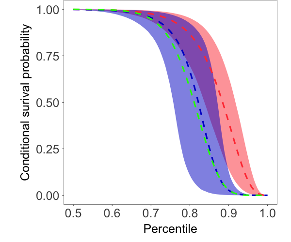
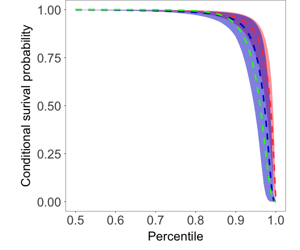
In this section, we demonstrate the use of copulas to construct NNMPs for tail dependence modeling. Our focus is on illustrating the flexibility of copula NNMPs for modeling complex dependence structures, and not specifically on extreme value modeling.
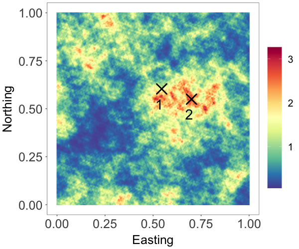
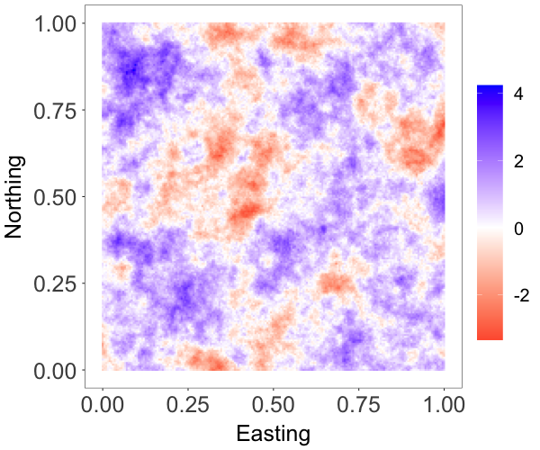
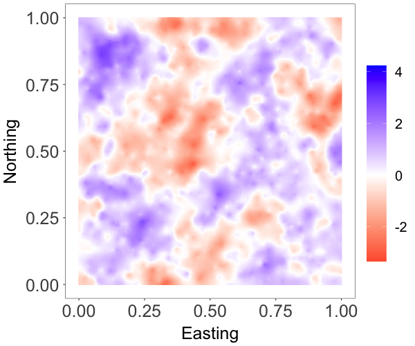
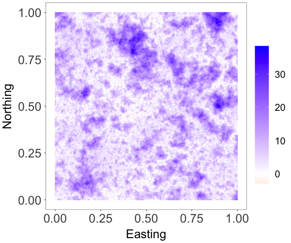
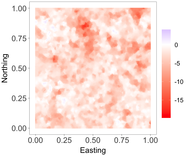
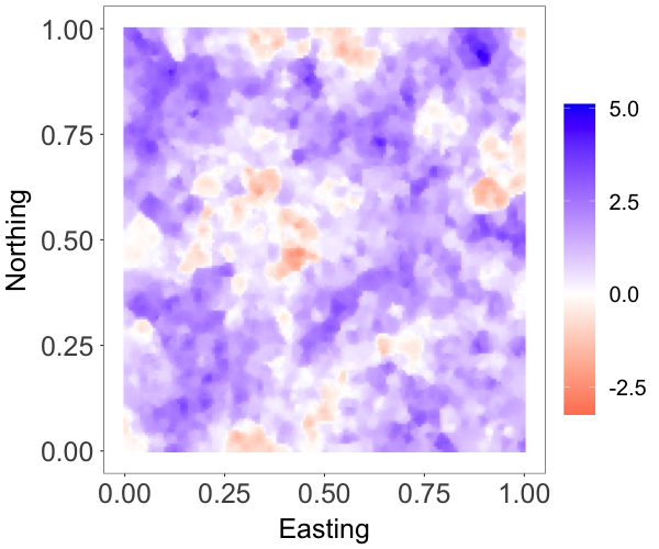
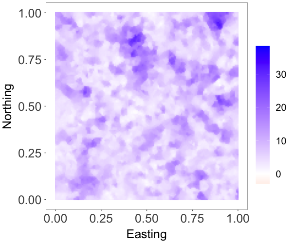
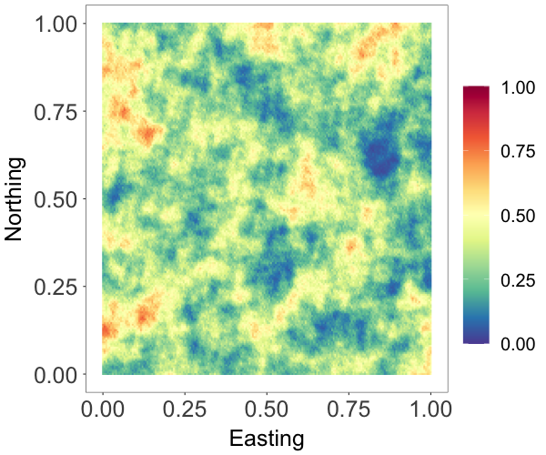
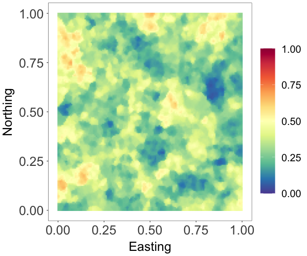
To simulate data, we created a regular grid of resolution on a unit
square domain , and generated over this grid a realization from random field
;
see Fig. 1(a). Here, is a standard Student-t process with tail parameter
and scale matrix specified by an exponential correlation function with range
parameter , and the distribution functions and correspond to
a gamma distribution, with mean , and a standard Student-t
distribution with tail parameter , respectively.
For a given pair of locations in with correlation ,
the corresponding tail dependence coefficient of the random field is
.
We took , and chose so that the synthetic data exhibits moderate tail
dependence at close distance, and the dependence decreases rapidly as the distance
becomes larger. In particular, for , we obtain
, respectively.
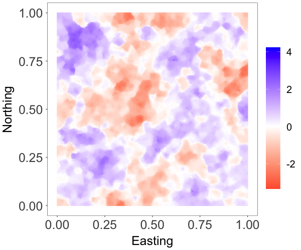
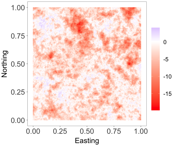
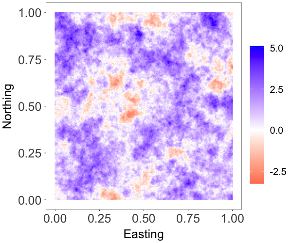
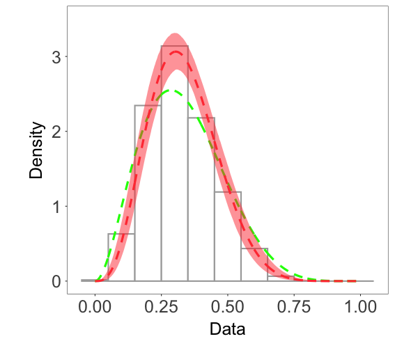
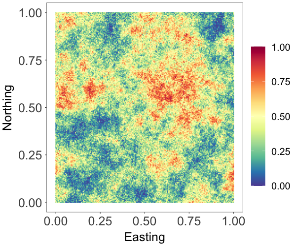
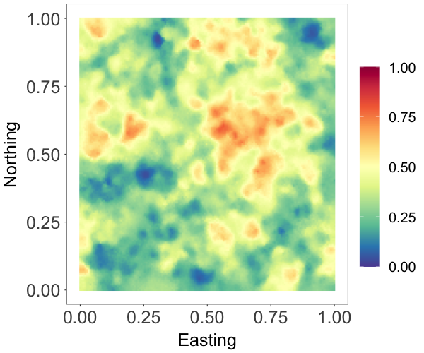
We applied two copula NNMP models. The models are of the form in (7) with stationary gamma marginal with mean . In the first model, the component copula density corresponds to a bivariate Gaussian copula, which is known to be unsuitable for tail dependence modeling. The spatially varying correlation parameter of the copula was specified by an exponential correlation function with range parameter . In the second model, we consider a spatially varying Gumbel copula as in Example 3. The spatially varying parameter of the copula density is defined with the link function , where the upper bound ensures numerical stability. When , . With this link function, we assume that given , the strength of the tail dependence with respect to the th component of the Gumbel model stays the same for any distance smaller than between two locations. For the cutoff point kernels, we specified an exponential correlation function with range parameters and , respectively, for each model. The Bayesian model is completed with a prior for and , a prior for and , a prior for and , and and priors.
We randomly selected 2000 locations as the reference set with a random ordering for model fitting. For the purposes of illustration, we chose neighbor size . Results are based on posterior samples collected every 10 iterations from a Markov chain of 30000 iterations, with the first 10000 samples being discarded. Implementation details for both models are provided in the supplementary material. The computing time was around minutes.
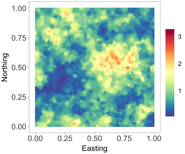
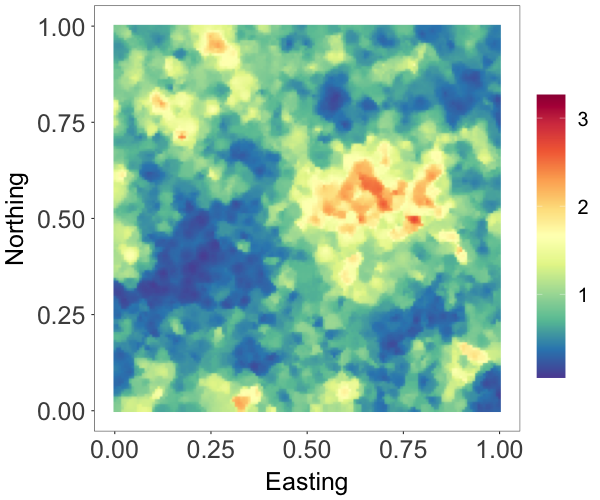
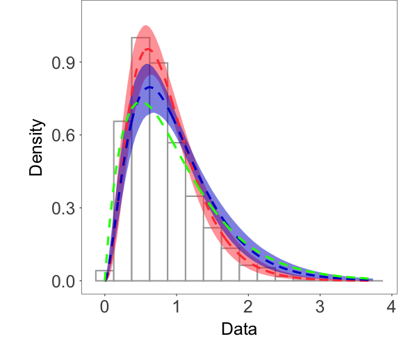
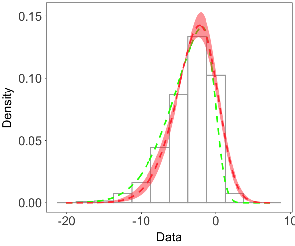
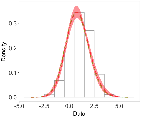
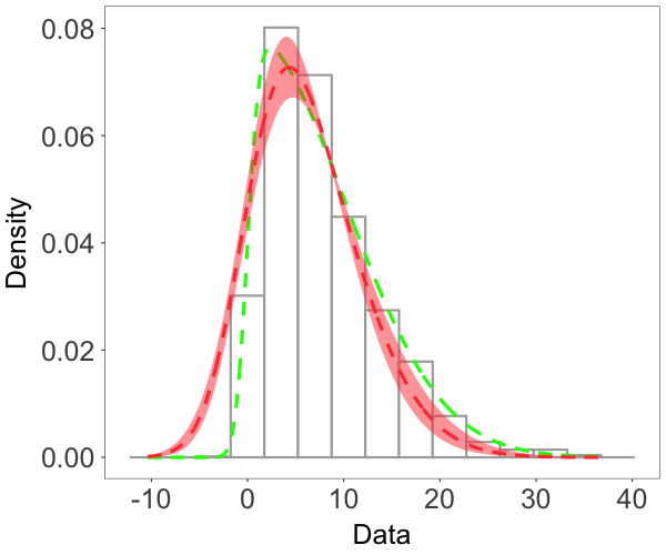
Fig. 1 shows the random fields, marginal densities, and conditional survival probabilities estimated by the two models. From Fig. 1(a)-1(c), we see that, comparing with the true field, the posterior median estimate by the Gumbel copula model seems to recover the large values better than the Gaussian copula model. Besides, as shown in Fig. 1(d), the Gumbel copula model provides a more accurate estimate of the marginal distribution, especially in the tails. We computed the conditional survival probabilities at two different unobserved sites marked in Fig. 1(a). In particular, Site 1/2 is surrounded by reference set observations with moderate/large values. The Gumbel copula model provides much more accurate estimates of the conditional survival probabilities, indicating that the model captures better the tail dependence structure in the data. Overall, this example demonstrates that the Gumbel copula NNMP model is a useful option for modeling spatial processes with tail dependence.
4.2 Mediterranean Sea Surface Temperature Data Analysis
The study of Ocean’s dynamics is crucial for understanding climate variability. One of the most valuable sources of information regarding the evolution of the state of the ocean is provided by the centuries-long record of temperature observations from the surface of the oceans. The record of sea surface temperatures consists of data collected over time at irregularly scattered locations. In this section, we examine the sea surface temperature from the Mediterranean Sea area during December 2003.
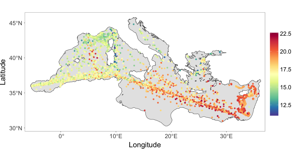
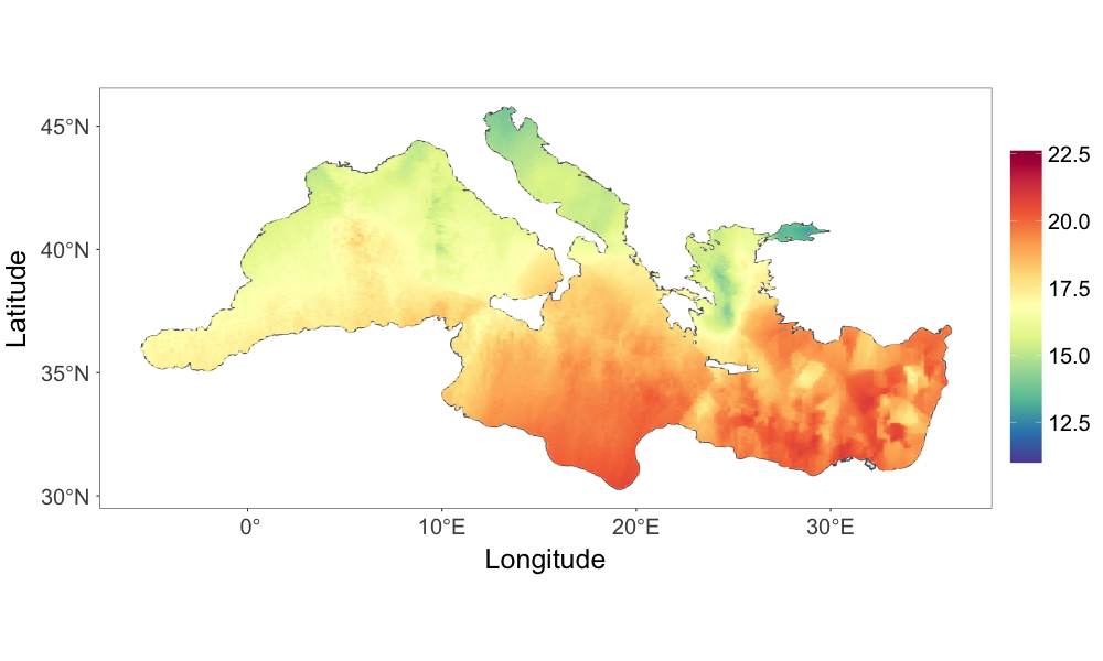
It is well known that the Mediterranean Sea area produces very heterogeneous temperature fields. A goal of the spatial analysis of sea surface temperature in the area is to generate a spatially continuous field that accounts for the complexity of the surrounding coastlines as well as the non-linear dynamics of the circulation system. An additional source of complexity comes from the data collection process. Historically, the observations are collected from different types of devices: buckets launched from navigating vessels, readings from the water intake of ships’ engine rooms, moored buoys, and drifting buoys (Kirsner and Sansó, 2020). The source of some observations is known, but not all the data are labelled. A thorough case study will be needed to include all this information in order to account for possible heterogeneities due to the different measuring devices. That is beyond the scope of this paper. We will focus on demonstrating the ability of the proposed framework to model non-Gaussian spatial processes that, hopefully, capture the complexities of the physical process and the data collection protocol. We notice that in the original record several sites had multiple observations. In those cases we took the median of the observations, resulting in a total of 1966 observations. The data are shown in Fig. 2(a).
We first examine the Gaussianity assumption for the data. We compare the Gaussian NNMP and the nearest-neighbor Gaussian process models over a subset of the region where the ocean dynamics are known to be complex and the observations are heterogeneous. The model comparison is detailed in the supplementary material and the results support the NNMP model.
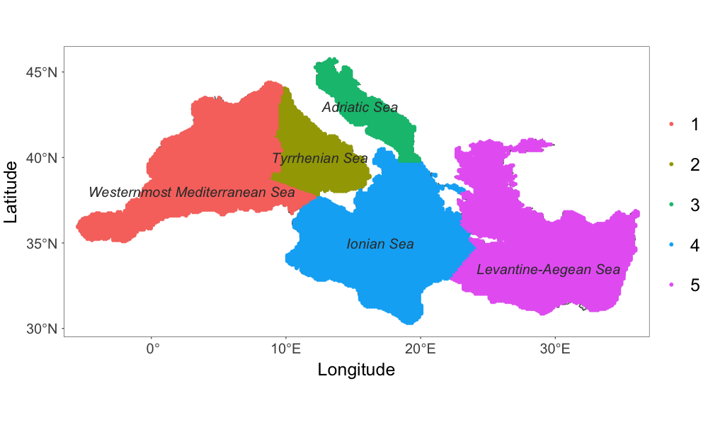
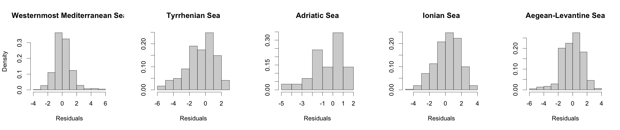
In light of the evidence (Pisano et al., 2020) that sea surface temperature spatial patterns are different over Mediterranean sub-basins, shown in Fig. 2(b), which are characterized by different dynamics and high variability of surface currents (Bouzaiene et al., 2020), we further investigate the sea surface temperature over those sub-basins. We fitted a non-spatial linear model to all data, including longitude and latitude as covariates, and obtained residuals from the linear model. Fig. 2(e) shows that the histograms of the residuals are asymmetric over the sub-basins, indicating skewness in the marginal distribution, with levels of skewness that vary across sub-basins.
The exploratory data analysis suggests the need for a spatial model that can capture skewness. We thus analyze the full data set with an extension of the skew-Gaussian NNMP model. The new model has two features that extend the skew-Gaussian NNMP: (i) it incorporates a fixed effect through the location parameter of the mixture component; (ii) it allows the skewness parameter to vary in space. More specifically, the spatially varying conditional density of the model builds from a Gaussian random vector with mean and covariance matrix , where and , for all and for all , and are longitude and latitude. The conditional density of the extended model is
| (10) |
with parameters , , , and . After marginalizing out , we obtain that the marginal distribution of is , based on the result of Proposition 1. We model the spatially varying via a partitioning approach. In particular, we partition the Mediterranean Sea according to the sub-basins, that is, , for , where . For all , we take , for . The partitions correspond to the sub-basins: Westernmost Mediterranean Sea, Tyrrhenian Sea, Adriatic Sea, Ionian Sea, and Levantine-Aegean Sea.
We applied the extended skew-Gaussian NNMP model (10) using the whole data set as the reference set, with chosen to be or . The regression parameters were assigned mean-zero, dispersed normal priors. For the skewness parameters , each element received a prior. We used the same prior specification for other parameters as in the first simulation experiment. Posterior inference was based on thinned samples retaining every 4th iteration, from a total of 30000 samples with a burn-in of 10000 samples. The computing time was around 14, 16, and 20 minutes, respectively, for each of the values.
We focus on the estimation of regression and skewness parameters and . We report the estimates for ; they were similar for or . The posterior mean and credible interval estimates of , , and were , , and , indicating that there was an increasing trend in sea surface temperature as longitude increased and latitude decreased. The corresponding posterior estimates of were , , , , and . These estimates suggest different levels of left skewness over the sub-basins except for the Westernmost Mediterranean Sea.
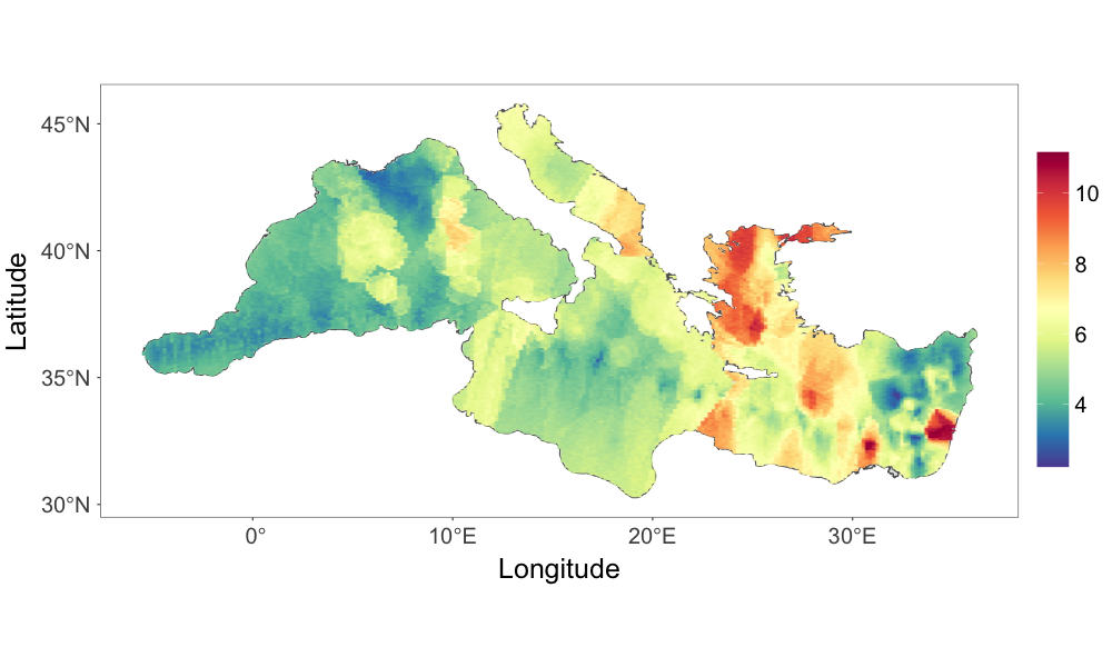
Fig. 2(c) provides the temperature posterior median estimate over a dense grid of locations on the Mediterranean Sea. Compared to Fig. 2(a), the estimate generally resembles the observed pattern. The prediction was quite smooth even for areas with few observations. The 95% credible interval width of the prediction over the gridded locations, as shown in Fig. 2(d), demonstrates that the model describes the uncertainty in accordance with the observed data structure; the uncertainty is higher in areas where there are less observations or the observations are volatile.
5 Discussion
We have introduced a class of geostatistical models for non-Gaussian processes, and demonstrated its flexibility for modeling complex dependence by specification of a collection of bivariate distributions indexed in space. The scope of the methodology has been illustrated through synthetic spatial data examples corresponding to distributions of different nature and support, and with the analysis of sea surface temperature measurements from the Mediterranean Sea.
To incorporate covariates, the NNMP can be embedded in an additive or multiplicative model. The former is illustrated in the supplementary material with a spatially varying regression model. Under an additive model, the posterior simulation algorithm requires extra care as it involves sequential updating of the elements in . This may induce slow convergence behavior. An alternative strategy for covariate inclusion is to model the weights or some parameter(s) of the spatially varying conditional density as a function of covariates. For example, in Section 4.2, we modeled the location parameter of the skew-Gaussian marginal as a linear function of the covariates. Posterior simulation under this approach is easily developed by modifying the update of the relevant parameters discussed in Section 3.2 to that of the regression coefficients.
The NNMP model structure not only bypasses all the potential issues from large matrix operations, but it also enhances modeling power. Kernel functions, such as wave covariance functions, that are impractical for Gaussian process-based models due to numerical instability from matrix inversion, can be used as link functions for the spatially varying parameter of the NNMP. One limitation of the NNMP’s computation, similar to mixture models, is that the posterior simulation algorithm may experience slow convergence issues. Further development is needed on efficient algorithms for fast computation, especially when dealing with massive, complex data sets.
We have focused in this article on a modeling framework for continuous data. The proposed approach can be naturally extended to modeling discrete spatial data. Modeling options for geostatistical count data in the existing literature involve either spatial generalized linear mixed models or spatial copula models (Madsen, 2009). However, owing to their structures, both models have limitations with respect to the distributional assumption for the spatial random effects, as well as in computational efficiency. The extension to discrete NNMP models has the potential to provide both inferential and computational benefits in modeling large discrete data sets.
It is also interesting to explore the opportunities for the analysis of spatial extremes using the NNMP framework. We developed guidelines in Section 2.4 to choose NNMP mixture components based on strength of tail dependence. The results highlight the ability of the NNMP model structure to capture local tail dependence at different levels, controlled by the mixture component bivariate distributions, for instance, with a class of bivariate extreme-value copulas. Moreover, using NNMPs for spatial extreme value modeling allows for efficient implementation of inference which is typically a challenge with existing approaches (Davison et al., 2012).
Other research directions include extensions to multivariate and spatio-temporal settings. The former extension requires families of high-dimensional multivariate distributions to construct an NNMP. Effective strategies will be needed to define the spatially varying multivariate distributions that balance flexibility and scalability. When it comes to a joint model over time and space, there is large scope for exploring the integration of the time component into the model, including extending the NNMP weights or the NNMP mixture components.
Supplementary Material
The supplementary material includes proofs of the propositions, additional data examples, and implementation details.
References
- Allcroft and Glasbey (2003) Allcroft, D. J. and Glasbey, C. A. (2003), “A latent Gaussian Markov random-field model for spatiotemporal rainfall disaggregation,” Journal of the Royal Statistical Society: Series C (Applied Statistics), 52, 487–498.
- Arnold et al. (1999) Arnold, B. C., Castillo, E., and Sarabia, J. M. (1999), Conditional specification of statistical models, New York: Springer.
- Azzalini (2013) Azzalini, A. (2013), The skew-normal and related families, Cambridge, UK: Cambridge University Press.
- Bárdossy (2006) Bárdossy, A. (2006), “Copula-based geostatistical models for groundwater quality parameters,” Water Resources Research, 42.
- Beck et al. (2020) Beck, N., Genest, C., Jalbert, J., and Mailhot, M. (2020), “Predicting extreme surges from sparse data using a copula-based hierarchical Bayesian spatial model,” Environmetrics, 31, e2616.
- Bevilacqua et al. (2021) Bevilacqua, M., Caamaño-Carrillo, C., Arellano-Valle, R. B., and Morales-Oñate, V. (2021), “Non-Gaussian geostatistical modeling using (skew) t processes,” Scandinavian Journal of Statistics, 48, 212–245.
- Bevilacqua et al. (2020) Bevilacqua, M., Caamaño-Carrillo, C., and Gaetan, C. (2020), “On modeling positive continuous data with spatiotemporal dependence,” Environmetrics, 31, e2632.
- Bolin (2014) Bolin, D. (2014), “Spatial Matérn fields driven by non-Gaussian noise,” Scandinavian Journal of Statistics, 41, 557–579.
- Bouzaiene et al. (2020) Bouzaiene, M., Menna, M., Poulain, P.-M., Bussani, A., and Elhmaidi, D. (2020), “Analysis of the Surface Dispersion in the Mediterranean Sub-Basins,” Frontiers in Marine Science, 7, 486.
- Cadonna et al. (2019) Cadonna, A., Kottas, A., and Prado, R. (2019), “Bayesian spectral modeling for multiple time series,” Journal of the American Statistical Association, 114, 1838–1853.
- Danaher and Smith (2011) Danaher, P. J. and Smith, M. S. (2011), “Modeling multivariate distributions using copulas: Applications in marketing,” Marketing Science, 30, 4–21.
- Datta et al. (2016a) Datta, A., Banerjee, S., Finley, A. O., and Gelfand, A. E. (2016a), “Hierarchical nearest-neighbor Gaussian process models for large geostatistical datasets,” Journal of the American Statistical Association, 111, 800–812.
- Datta et al. (2016b) Datta, A., Banerjee, S., Finley, A. O., Hamm, N. A., and Schaap, M. (2016b), “Nonseparable dynamic nearest neighbor Gaussian process models for large spatio-temporal data with an application to particulate matter analysis,” The Annals of Applied Statistics, 10, 1286.
- Davison et al. (2012) Davison, A. C., Padoan, S. A., and Ribatet, M. (2012), “Statistical modeling of spatial extremes,” Statistical science, 27, 161–186.
- De Oliveira et al. (1997) De Oliveira, V., Kedem, B., and Short, D. A. (1997), “Bayesian prediction of transformed Gaussian random fields,” Journal of the American Statistical Association, 92, 1422–1433.
- Diggle et al. (1998) Diggle, P. J., Tawn, J. A., and Moyeed, R. A. (1998), “Model-based geostatistics,” Journal of the Royal Statistical Society: Series C (Applied Statistics), 47, 299–350.
- Eskelson et al. (2011) Eskelson, B. N., Madsen, L., Hagar, J. C., and Temesgen, H. (2011), “Estimating riparian understory vegetation cover with beta regression and copula models,” Forest Science, 57, 212–221.
- Ferguson (1973) Ferguson, T. S. (1973), “A Bayesian analysis of some nonparametric problems,” The Annals of Statistics, 209–230.
- Finley et al. (2019) Finley, A. O., Datta, A., Cook, B. D., Morton, D. C., Andersen, H. E., and Banerjee, S. (2019), “Efficient algorithms for Bayesian nearest neighbor Gaussian processes,” Journal of Computational and Graphical Statistics, 28, 401–414.
- Gelfand et al. (2005) Gelfand, A. E., Kottas, A., and MacEachern, S. N. (2005), “Bayesian nonparametric spatial modeling with Dirichlet process mixing,” Journal of the American Statistical Association, 100, 1021–1035.
- Ghosh and Mallick (2011) Ghosh, S. and Mallick, B. K. (2011), “A hierarchical Bayesian spatio-temporal model for extreme precipitation events,” Environmetrics, 22, 192–204.
- Gräler (2014) Gräler, B. (2014), “Modelling skewed spatial random fields through the spatial vine copula,” Spatial Statistics, 10, 87–102.
- Gramacy and Apley (2015) Gramacy, R. B. and Apley, D. W. (2015), “Local Gaussian process approximation for large computer experiments,” Journal of Computational and Graphical Statistics, 24, 561–578.
- Guinness (2018) Guinness, J. (2018), “Permutation and grouping methods for sharpening Gaussian process approximations,” Technometrics, 60, 415–429.
- Hua and Joe (2014) Hua, L. and Joe, H. (2014), “Strength of tail dependence based on conditional tail expectation,” Journal of Multivariate Analysis, 123, 143–159.
- Joe (2014) Joe, H. (2014), Dependence modeling with copulas, Boca Raton, FL: CRC Press.
- Johns et al. (2003) Johns, C. J., Nychka, D., Kittel, T. G. F., and Daly, C. (2003), “Infilling sparse records of spatial fields,” Journal of the American Statistical Association, 98, 796–806.
- Katzfuss and Guinness (2021) Katzfuss, M. and Guinness, J. (2021), “A general framework for Vecchia approximations of Gaussian processes,” Statistical Science, 36, 124–141.
- Kim and Mallick (2004) Kim, H.-M. and Mallick, B. K. (2004), “A Bayesian prediction using the skew Gaussian distribution,” Journal of Statistical Planning and Inference, 120, 85–101.
- Kirsner and Sansó (2020) Kirsner, D. and Sansó, B. (2020), “Multi-scale shotgun stochastic search for large spatial datasets,” Computational Statistics & Data Analysis, 146, 106931.
- Krupskii et al. (2018) Krupskii, P., Huser, R., and Genton, M. G. (2018), “Factor copula models for replicated spatial data,” Journal of the American Statistical Association, 113, 467–479.
- Lauritzen (1996) Lauritzen, S. L. (1996), Graphical models, Oxford, UK: Clarendon Press.
- Le et al. (1996) Le, N. D., Martin, R. D., and Raftery, A. E. (1996), “Modeling flat stretches, bursts outliers in time series using mixture transition distribution models,” Journal of the American Statistical Association, 91, 1504–1515.
- Madsen (2009) Madsen, L. (2009), “Maximum likelihood estimation of regression parameters with spatially dependent discrete data,” Journal of Agricultural, Biological, and Environmental Statistics, 14, 375–391.
- Mahmoudian (2017) Mahmoudian, B. (2017), “A skewed and heavy-tailed latent random field model for spatial extremes,” Journal of Computational and Graphical Statistics, 26, 658–670.
- Morris et al. (2017) Morris, S. A., Reich, B. J., Thibaud, E., and Cooley, D. (2017), “A space-time skew-t model for threshold exceedances,” Biometrics, 73, 749–758.
- Müller et al. (2018) Müller, P., Quintana, F. A., and Page, G. (2018), “Nonparametric Bayesian inference in applications,” Statistical Methods & Applications, 27, 175–206.
- North et al. (2011) North, G. R., Wang, J., and Genton, M. G. (2011), “Correlation models for temperature fields,” Journal of Climate, 24, 5850–5862.
- Palacios and Steel (2006) Palacios, M. B. and Steel, M. F. J. (2006), “Non-Gaussian Bayesian geostatistical modeling,” Journal of the American Statistical Association, 101, 604–618.
- Peruzzi et al. (2020) Peruzzi, M., Banerjee, S., and Finley, A. O. (2020), “Highly Scalable Bayesian Geostatistical Modeling via Meshed Gaussian Processes on Partitioned Domains,” Journal of the American Statistical Association, 0, 1–14.
- Peruzzi and Dunson (2022) Peruzzi, M. and Dunson, D. B. (2022), “Spatial Multivariate Trees for Big Data Bayesian Regression.” Journal of Machine Learning Research, 23, 17–1.
- Pisano et al. (2020) Pisano, A., Marullo, S., Artale, V., Falcini, F., Yang, C., Leonelli, F. E., Santoleri, R., and Buongiorno Nardelli, B. (2020), “New evidence of Mediterranean climate change and variability from sea surface temperature observations,” Remote Sensing, 12, 132.
- Sklar (1959) Sklar, M. (1959), “Fonctions de repartition an dimensions et leurs marges,” Publications de l’Institut de Statistique de L’Université de Paris, 8, 229–231.
- Stein et al. (2004) Stein, M. L., Chi, Z., and Welty, L. J. (2004), “Approximating likelihoods for large spatial data sets,” Journal of the Royal Statistical Society: Series B (Statistical Methodology), 66, 275–296.
- Sun et al. (2015) Sun, Y., Stein, M. L., et al. (2015), “A stochastic space-time model for intermittent precipitation occurrences,” The Annals of Applied Statistics, 9, 2110–2132.
- Vecchia (1988) Vecchia, A. V. (1988), “Estimation and model identification for continuous spatial processes,” Journal of the Royal Statistical Society: Series B (Methodological), 50, 297–312.
- Wallin and Bolin (2015) Wallin, J. and Bolin, D. (2015), “Geostatistical modelling using non-Gaussian Matérn fields,” Scandinavian Journal of Statistics, 42, 872–890.
- Xu and Genton (2017) Xu, G. and Genton, M. G. (2017), “Tukey g-and-h random fields,” Journal of the American Statistical Association, 112, 1236–1249.
- Zareifard et al. (2018) Zareifard, H., Khaledi, M. J., Rivaz, F., Vahidi-Asl, M. Q., et al. (2018), “Modeling skewed spatial data using a convolution of Gaussian and log-Gaussian processes,” Bayesian Analysis, 13, 531–557.
- Zhang and El-Shaarawi (2010) Zhang, H. and El-Shaarawi, A. (2010), “On spatial skew-Gaussian processes and applications,” Environmetrics, 21, 33–47.
- Zheng et al. (2022) Zheng, X., Kottas, A., and Sansó, B. (2022), “On Construction and Estimation of Stationary Mixture Transition Distribution Models,” Journal of Computational and Graphical Statistics, 31, 283–293.
- Zilber and Katzfuss (2021) Zilber, D. and Katzfuss, M. (2021), “Vecchia–Laplace approximations of generalized Gaussian processes for big non-Gaussian spatial data,” Computational Statistics & Data Analysis, 153, 107081.
Supplementary Material for “Nearest-Neighbor Mixture Models for Non-Gaussian Spatial Processes”
A Proofs
Proof of Proposition 1.
We consider a univariate spatial process , where takes values in , and . Let be a reference set. Without loss of generality, we consider the continuous case, i.e., has a continuous distribution for which its density exists, for all . To verify the proposition, we partition the domain into the reference set and the nonreference set .
Given any , consider a bivariate random vector indexed at , denoted as taking values in . We denote as the conditional density of given , and as the marginal densities of , , respectively. Using the proposition assumption that , we have that
| (1) |
for every and for all .
We first prove the result for the reference set . By the model assumption, locations in are ordered. In this regard, using the proposition assumptions, we can show that for all by applying Proposition 1 in (Zheng et al., 2022).
Turning to the nonreference set . Let be the marginal density of for every . Denote by the joint density for the random vector where , so every element of has marginal density . Then, the marginal density for is given by:
where the second-to-last equality holds by the result that for all and for every . The last equality follows from (1).
∎
Proof of Proposition 2.
We verify the proposition by partitioning the domain into the reference set and the nonreference set . We first prove by induction the result for the joint distribution over . Then to complete the proof, it suffices to show that for every location , the joint density is a mixture of multivariate Gaussian distributions, where .
Without loss of generality, we assume for the stationary Gaussian NNMP, i.e., the Gaussian NNMP has invariant marginal . The conditional density for the reference set is , where for, , , and for , . For each , we denote as the vector of mixture weights, as the vector of the correlation coefficients, and as the vector of the nearest neighbors of , for , where , , . Let . We denote by the realization of over locations for , and use to denote the random vector with element removed, . In the following, for a vector , we have that , where is a scalar.
Take . When , and . The joint density of is , where . The joint density of is
where , and . The last equality follows from the fact that a product of conditionally independent Gaussian densities is a Gaussian density. By the properties of the Gaussian distribution and the property of the model that has a stationary marginal , for each , we have that
where , with the following partition relevant to the vector ,
where corresponds to . It follows that
| (2) | ||||
From (2), we obtain and for . Then we reorder with a matrix such that . It follows that , and the joint density is .
Similarly, the joint density of is given by
where , and is a rotation matrix such that . We partition the matrix such that and correspond to and , respectively. We have that for ,
and
We reorder with matrix such that and let . Then we obtain the joint density of as .
Applying the above technique iteratively for for , we obtain the joint density , for , namely,
where , , and for ,
where is the rotation matrix such that , and is the rotation matrix such that the vector , where .
To complete the proof, what remains to be shown is that the density is a mixture of multivariate Gaussian distributions, where . We have that , where is an element of for . We can express each component density of the joint density as the product of a Gaussian density of conditional on and a Gaussian density of . Using the approach in deriving the joint density over , we can show that is a mixture of multivariate Gaussian distributions.
∎
Proof of Proposition 3.
For an NNMP , the conditional probability that is greater than given its neighbors , where , is , where the conditional probability corresponds to the bivariate random vector . If is stochastically increasing in for all , by the assumption that the sequence is built from the base random vectors for all , we have that is stochastically increasing in for every , i.e., , for all and in the support of , such that for all .
Let and be the distribution functions of and , respectively. Denote by the joint survival probability. Then for every and ,
| (3) | ||||
where the inequality follows the assumption of stochastically increasing positive dependence of given .
Taking on both sides of (3), we obtain , where and are the marginal distribution functions of . Similarly, we can obtain the lower bound for .
∎
Proof of Corollary 1.
We prove the result for . The result for is obtained in a similar way. Consider a bivariate cdf for random vector , with marginal cdfs and marginal densities , for all . The lower tail dependence coefficient is expressed as with . If has first order partial derivatives, applying the L’Hopital’s rule, we obtain
The above is a reproduced result from Theorem 8.57 of (Joe, 2014). If is exchangeable, we have . If the sequences of an NNMP model are built from the base random vectors . By our assumption that for all , the marginal cdfs of extended from are for all and all . Then we have . Using the result of Proposition 3, we obtain
∎
Proof of Proposition 4.
By the assumption that is stochastically increasing in and that is constructed based on , is stochastically increasing in for all and for all . Then for with respect to the bivariate distribution of with marginal distributions and , we have that
It follows that the boundary cdf of the NNMP model
| (4) | ||||
Taking on both sides of (4), we obtain . If there exists some such that , then has strictly positive mass at . Similarly, we can prove the result for .
∎
B Additional Data Illustrations
We provide three additional simulation experiments to demonstrate the benefits of the proposed NNMP framework. The first simulation experiment demonstrates that the Gaussian NNMP (GNNMP) provides a good approximation to Gaussian random fields. The second example illustrates the ability of the framework to handle skewed data using a skew-Gaussian NNMP (skew-GNNMP) model. Next, we demonstrate the effectiveness of the NNMP model for bounded spatial data. The last part of this section examines the non-Gaussian process assumption for the analysis of Mediterranean Sea surface temperature data example presented in the main paper, using a limited region to compare the GNNMP and the nearest-neighbor Gaussian process (NNGP) models.
In each of the experiments, we created a regular grid of resolution on a unit square domain, and generated data on each grid location. We then randomly selected a subset of the data as the reference set with a random ordering for model fitting. For the purpose of illustration, we chose neighbor size for both cases. Results are based on posterior samples collected every 10 iterations from a Markov chain of 30000 iterations, with the first 10000 samples as a burn-in.
B.1 Additional Simulation Experiment 1
We generated data from a spatially varying regression, , where is a standard Gaussian process with an exponential correlation function with range parameter . We included an intercept and a covariate drawn from in the model, and chose , and . The setting followed the simulation experiment in Datta et al. (2016a).
We applied two models. The first one assumes that follows an NNGP model with variance and exponential correlation function with range parameter . The second one assumes that follows a stationary GNNMP model, i.e., and for all , such that has a stationary marginal . For the GNNMP, we used exponential correlation functions with range parameter and , respectively, for the correlation with respect to the component density and the cutoff points kernel function. For the NNGP model, we implement the latent NNGP algorithm from the spNNGP package in R \citepsmspnngp. We trained both models using 2000 of the 2500 observations, and used the remaining 500 observations for model comparison.
For both models, the regression coefficients were assigned flat priors. The variances and received the same inverse gamma prior , and was assigned . The range parameter of the NNGP received a uniform prior , while the range parameters and of the GNNMP received inverse gamma priors and , respectively. Regarding the logit Gaussian distribution parameters, and , we used and priors, respectively.
The posterior estimates from the two models for the common parameters, and , were quite close. The posterior mean and credible interval estimates of and were and from the GNNMP model, and and from the NNGP model. The corresponding estimates of were and from the GNNMP and NNMP models, respectively.
| RMSPE | 95% CI | 95% CI width | CRPS | PPLC | DIC | |
|---|---|---|---|---|---|---|
| GNNMP | 0.57 | 0.96 | 2.51 | 0.32 | 461.40 | 2656.67 |
| NNGP | 0.54 | 0.95 | 2.09 | 0.30 | 382.15 | 2268.79 |
Table 1 shows the performance metrics of the two models. The performance metrics of the GNNMP model are comparable to those of the NNGP model, the model assumptions of which are more well suited to the particular synthetic data example. The posterior median estimate of the spatial random effects from both models are shown in Figure 1. We can see that the predictive field given by the GNNMP looks close to the true field and that predicted by the NNGP. On the whole, the GNNMP model provides a reasonably good approximation to the Gaussian random field.
B.2 Additional Simulation Experiment 2
We generated data from the skew-Gaussian process (Zhang and El-Shaarawi, 2010),
| (5) |
where and are both standard Gaussian processes with correlation matrix specified by an exponential correlation function with range parameter . The parameter controls the skewness, whereas is a scale parameter. The model has a stationary skew-Gaussian marginal density . We took , and generated data with , and , resulting in three different random fields that are, respectively, moderately negative-skewed, slightly positive-skewed, and strongly positive-skewed, as shown in Figure 2(a)-2(c).
We applied the stationary skew-GNNMP model. The model is obtained as a special case of the skew-GNNMP model discussed in Section 2.3 of the main paper, taking , , and , for all . Here, controls the skewness, such that a large positive (negative) value of indicates strong positive (negative) skewness. If , the skew-GNNMP model reduces to the GNNMP model. After marginalizing out , we obtain a stationary skew-Gaussian marginal density . We completed the full Bayesian specification for the model, by assigning priors , , , , , and , where is the range parameter of the exponential correlation function specified for the cutoff point kernel.
We focus on the model performance on capturing skewness . The posterior mean and 95% credible interval of for the three scenarios were , and , respectively, indicating the model’s ability to estimate different levels of skewness. The bottom row of Figure 2 shows that the posterior median estimates of the surfaces capture well features of the true surfaces, even when the level of skewness is small, thus demonstrating that the model is also able to recover near-Gaussian features. Figure 3 plots the posterior mean and pointwise 95% credible interval for the marginal density, overlaid on the histogram of the simulated data for each of the three cases. These estimates demonstrate the adaptability of the skew-GNNMP model in capturing skewed random fields with different levels of skewness.
B.3 Additional Simulation Experiment 3
Many spatial processes are measured over a compact interval. As an example, data on proportions are common in ecological applications. In this experiment, we demonstrate the effectiveness of the NNMP model for directly modeling bounded spatial data. We generated data using the model , where the cdf corresponds to a beta distribution, denoted as , and is a standard Gaussian process with exponential correlation function with range parameter . We set , .
We applied a Gaussian copula NNMP model with stationary marginal , with the same spatial Gaussian copula and prior specification used in the second experiment. We used 2000 observations to train the model. Figure 4(b) shows the estimated random field which captures well the main features of the true field in Figure 4(a). The posterior mean and pointwise credible interval of the estimated marginal density in Figure 4(c) overlay on the data histogram. These show that the beta NNMP estimation and prediction provide good approximation to the true field.
It is worth mentioning that implementing the beta NNMP model is simpler than fitting existing models for data corresponding to proportions. For example, a spatial Gaussian copula model, that corresponds to the data generating process of this experiment, involves computations for large matrices. Alternatively, if a multivariate non-Gaussian copula is used, the resulting likelihood can be intractable and require certain approximations. Another model that is commonly used in this setting is defined analogously to a spatial generalized linear mixed model. The spatial element in the model is introduced through the transformed mean of the observations. A sample-based approach to fit such a model requires sampling a large number of highly correlated latent variables. We conducted an experiment to demonstrate the effectiveness of the beta NNMP to approximate random fields simulated by the link function approach. We generated data as follows.
The above model is analogous to a spatial generalized linear mixed model where the mean of the beta distribution is modeled via a logit link function, and is a standard Gaussian process with exponential correlation function with range parameter . We set , and .
Since our purpose is primarily demonstrative, we applied a Gaussian copula NNMP model with a stationary beta marginal , referred to as the beta NNMP model. The correlation parameter of the Gaussian copula was specified by an exponential correlation function with range parameter . We specified an exponential correlation function for the random cutoff points kernel function with range parameter . The Bayesian model is fully specified with a prior for , a prior for and , a prior for , and .
We trained the model using 2000 observations. Figure 5(a)-(b) shows the interpolated surface of the true field and the predictive field given by the beta NNMP model. Although the beta NNMP’s stationary marginal distribution assumption does not align with the true model, we can see that the predictive filed was able to capture the main feature of the true field. Moreover, it is worth mentioning that the MCMC algorithm for the beta NNMP to fit the data set took around 18 minutes with 30000 iterations. This is substantially faster than the MCMC algorithm for fitting the true model which involves sampling a large number of highly correlated latent variables.
B.4 Mediterranean Sea Surface Temperature Regional Analysis
In this section, we examine the non-Gaussian process assumption for the Mediterranean Sea surface temperature data. We focus on sea surface temperature (SST) over an area near the Gulf of Lion, along the islands near the shores of Spain, France, Monaco and Italy, between 0 - 9 E. longitude and 33.5 - 44.5 N. latitude. The SST observations in the region, as shown in Figure 6(a), are very heterogeneous, implying that the short range variability can be non-Gaussian. We compare the GNNMP with the NNGP in a spatially varying regression model, demonstrating the benefit of using a non-Gaussian process to explain the SST variability. In particular, the GNNMP has the same Gaussian marginals as the NNGP, but its finite-dimensional distribution is a mixture of Gaussian distributions.
We consider the following spatially varying regression model,
| (6) |
where is the SST observation, includes longitude and latitude to account for the long range variability in SST with regression parameters , is a spatial process, and represents the micro-scale variability and/or the measurement error.
We model with the GNNMP defined in (7) with and , for all . For comparison, we also applied an NNGP model for with variance and exponential correlation function with range parameter . For the GNNMP, we used exponential correlation functions with range parameter and , respectively, for the correlation with respect to the component density, and the cutoff point kernel. For both models, the regression coefficients were assigned flat priors. The variances and received the same inverse gamma prior , and was assigned . The range parameter of the NNGP received a uniform prior , while the range parameters and of the GNNMP received inverse gamma priors and , respectively. Regarding the logit Gaussian distribution parameters, and , we used and priors, respectively.
We took around 10% of the data in the region, as the held-out data for model comparison, and used the remaining 580 observations to train models. We compare models based on RMSPE, 95% posterior credible interval coverage rate (95% CI coverage), deviance information criterion (DIC; \citealtsmspiegelhalter2002bayesian), PPLC \citepsmgelfand1998model, and continuous ranked probability score (CRPS; \citealtsmgneiting2007strictly). To effectively compare the GNNMP and NNGP models, we first trained the NNGP model with neighbor sizes from 5 to 20, and selected the optimal neighbor size, that corresponds to the smallest RMSPE. We then trained the GNNMP model with the same . In all cases, we ran the MCMC with 120000 iterations, discarding the first 20000 samples, and collected samples every 20 iterations. The computing time was around 12 and 9 minutes for the GNNMP and NNGP models, respectively.
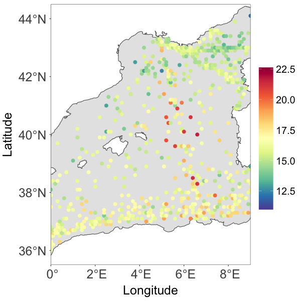
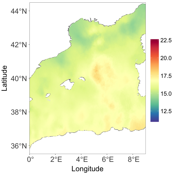

| RMSPE | 95% CI coverage | 95% CI width | CRPS | PPLC | DIC | |
|---|---|---|---|---|---|---|
| GNNMP | 0.92 | 0.97 | 4.09 | 0.50 | 135.58 | 539.53 |
| NNGP | 1.00 | 0.97 | 4.30 | 0.56 | 526.81 | 1083.61 |
We report the results for both models. The posterior mean and credible interval estimates of the regression intercept from the GNNMP was higher than the NNGP. They were and , respectively. The corresponding posterior estimates of the coefficients for longitude and latitude given by the GNNMP and the NNGP were and , respectively. Both models indicated that there was a trend of SST decreasing in the latitude at the selected region. For the error variance , the GNNMP provided a smaller estimate , compared to from the NNGP.
Regarding the model performance metrics in Table 2, both the PPLC and DIC suggest that the GNNMP had a better goodness-of-fit than the NNGP. For out-of-sample prediction, the GNNMP produced smaller RMSPE and CRPS than the NNGP. Both models gave the same 95% CI coverage, while the one from GNNMP had a narrower width. Figure 6(b)-6(c) show the posterior median estimates of the temperature field from both models. We can see that both models yield estimates that resemble the pattern in the observations. The predictive surface produced by the NNGP depicts some very localized, unrealistic features. These are not present in the results from the GNNMP.
C Implementation Details
We provide model implementation details for the data examples. In particular, Section C.1 corresponds to the GNNMP model applied in Sections B.1 and B.4. Section C.2 discusses the stationary skew-GNNMP model for the data example in Section B.2, and the extended skew-GNNMP model for the Mediterranean Sea surface data analysis of the main paper. Section C.3 introduces the Gaussian and Gumbel copula NNMP models implemented for the data example in Section B.3, and the simulation study of the main paper.
C.1 GNNMP Models
We consider the spatially varying regression model, , where , and the spatial random effect follows a stationary GNNMP model. The associated conditional density of the model is
| (7) |
where . For the weights, we consider an exponential correlation function with range parameter for the kernel function that defines the random cutoff points. The Bayesian model is completed with priors , , , , , , .
Let , , be the observations over reference set . We introduce the MCMC sampler. It involves sampling the latent variables , but it is easily developed based on the algorithm described in the main paper. For each , , we introduce a configuration variable , taking values in where , such that , where and if and otherwise. To allow for efficient simulation of parameters and for the weights, we associate each with a latent Gaussian variable with mean and variance , where , for . There is a one-to-one correspondence between the configuration variables and latent variables : if and only if where , for . The posterior distribution of the model parameters is given by
where the vector , and the matrix is such that the th row is .
We describe the MCMC sampler to simulate from the posterior distribution of model parameters and latent variables . Denote by , , and let be the covariate matrix with the th row being . The posterior full conditional distribution for is where and . An inverse gamma prior for yields an posterior full conditional, where .
To update the parameter , we first marginalize out the latent variables from the joint posterior distribution. The posterior full conditional distribution of is proportional to . We update on its log scale using a random walk Metropolis step. The posterior full conditional distribution of is , where and , for . Hence, each can be readily updated by sampling from the -th truncated Gaussian with probability proportional to . The posterior full conditional distribution of is where and . The posterior full conditional distribution of is .
The posterior full conditional distribution of is . The posterior full conditional distribution of is proportional to . We update on its log scale with a random walk Metropolis step. Denote by , and assume for every . The posterior full conditional of the latent spatial random effects is where and with , for .
C.2 Skew-GNNMP Models
C.2.1 Bivariate Skew-Gaussian Distribution
Exploiting the location mixture representation of the skew-Gaussian distribution \citepsmazzalini1996multivariate for bivariate random vector , we can write
| (8) |
It follows that, conditional on , the marginal densities of are and , respectively. Then the conditional density of given is . Therefore, the conditional density is a Gaussian distribution with mean and variance , truncated at , denoted as . Then the conditional distribution of given can be written as
| (9) |
where , .
Let and . After marginalizing out , the joint density of is given by , where , , and is the cdf of a standard Gaussian distribution. The marginal density of is , where and . We denote as . Similarly, the marginal density of is . It follows that the conditional density of given is
| (10) |
where , , , , and .
In the special case where and , let and . The joint density of can be written as , where the marginal density of is . The conditional density of given is then given by
| (11) |
where , , , and .
C.2.2 Stationary Skew-GNNMP Models
We take a set of base random vectors for all , where is a bivariate skew-Gaussian vector with distribution given by (8), and take , . We then extend to by extending to using an exponential correlation function such that , for . Using the resulting bivariate distribution for , we define the spatially varying density based on the formulation in (9). The resulting associated conditional density of the stationary skew-GNNMP is
| (12) |
where , , , and .
The component conditional density in (12) is sampled via a latent variable . We marginalize out to facilitate computation. Based on (11), we obtain the associated conditional density of the skew-GNNMP as
| (13) |
where , , , , , and . For the weights , we use an exponential correlation function with range parameter for the kernel functions of the random cutoff points. The Bayesian model is completed with prior specifications for . In particular, we consider priors , , , , and .
Given observations , , over reference set , we perform Bayesian inference based a likelihood conditional on the first observations. The posterior distribution of the model parameters, given the conditional likelihood, is given by
where the vector , and the matrix is such that the th row is .
The MCMC sampler to obtain samples from the joint posterior distribution is described in the main paper. We present the posterior updates of and . Note that the configuration variables are such that if for . Denote by . We use a random walk Metropolis step to update with target density . The posterior full conditional distributions of and are proportional to , and , respectively. For each parameter, we update it on its log scale with a random walk Metropolis step.
C.2.3 Extended Skew-GNNMP Models
Again, we take a set of base random vectors for all , where is a bivariate skew-Gaussian vector with distribution given by (8). We extend to by extending to using an exponential correlation function such that , and extending , , to , and to , for . Using the resulting bivariate distribution for , we define the spatially varying density based on the formulation in (9). The resulting associated conditional density of the extended skew-GNNMP is
| (14) |
where , , , and . After marginalizing out , the conditional density (14) based on formulation (10) can be written as
| (15) |
where , , , , , , and
We model the spatially varying via a partitioning approach. In particular, we partition the domain such that , for . For all , we take , for . For the weights , we use an exponential correlation function with range parameter for the kernel function of the random cutoff points. The Bayesian model is completed with prior specifications for . We assign a to the regression parameter and to , for . For other parameters, we take , , , and .
Given observations , , over reference set , we perform Bayesian inference based a likelihood conditional on the first observations. The posterior distribution of the model parameters is
where the vector , and the matrix is such that the th row is .
The MCMC sampler to obtain samples from the joint posterior distribution is described in the main paper. We present the posterior updates of and . Note that the configuration variables are such that if for . Denote by . We use a random walk Metropolis step to update with target density . Let . The posterior full conditional of is proportional to , and we use a random walk Metropolis step to sample , for . The posterior full conditional distributions of and are proportional to , and , respectively. For each parameter, we update it on its log scale with a random walk Metropolis step.
C.3 Copula NNMP Models
C.3.1 Gaussian and Gumbel Copulas
We consider a continuous bivariate vector with marginal cdfs and such that and . We introduce basic properties of the Gaussian and Gumbel copulas. For more details we refer to Joe (2014).
Gaussian copula
A Gaussian copula with correlation parameter for is , where is the cdf of a standard bivariate Gaussian distribution with correlation . The copula is asymptotically independent in both the lower and the upper tails. The corresponding copula density is
| (16) |
Denote by the conditional cdf of given . Then we have . We sample , given , with the following steps. Given a realization of , we compute . We then generate a random number from a uniform distribution on , and compute where is the inverse of . Finally, we obtain from the inverse cdf .
Gumbel copula
A Gumbel copula with parameter is . It is asymptotically independent in the lower tail and asymptotically dependent in the upper tail with tail dependence coefficient . The corresponding copula density is
| (17) |
Let and . In particular, the Gumbel copula can be written as , which is a bivariate exponential survival function, with marginals corresponding to a unit rate exponential distribution. The conditional cdf of given is . The inverse conditional cdf does not have a closed form. To generate given , following Joe (2014), we first define . Then we have a realization of , say , where is the root of , where , and is a random number generated from a uniform distribution on .
C.3.2 Copula NNMP Models and Inference
We take a set of base random vectors where its bivariate distribution is specified by a Gaussian copula with correlation parameter . We extend to by extending to , creating a sequence of spatially varying Gaussian copula for with marginal cdfs for all and all . The cdf corresponds to the stationary marginal distribution of the model. The associated conditional density of the Gaussian copula NNMP is
where is the Gaussian copula density obtained by replacing in (16) with , and is the density of .
Similarly, we can obtain the Gumbel copula NNMP model using a collection of spatially varying Gumbel copulas by extending in (17) to , where the upper bound ensures numerical stability.
We discuss the inferential approach for the Gaussian copula NNMP; the approach for the Gumbel copula NNMP model is similar. Assume the stationary marginal density is a gamma density, denoted as , with mean . For the weights , we use an exponential correlation function with range parameter to define the random cutoff points. The Bayesian model is completed with prior specifications for . In particular, we consider priors , , , , and .
Given observations , over reference set , we perform Bayesian inference using a likelihood conditional on . The posterior distribution of the model parameters is
where the vector , and the matrix is such that the th row is . We provide the updates for parameters . Note that the configuration variables are such that if for . Denote by . The posterior full conditional distributions for parameters , and are proportional to , , and , respectively. Each parameter is updated on its log scale with a random walk Metropolis step.
jasa3 \bibliographysmref