Nested adaptation of MCMC algorithms
Abstract
Markov chain Monte Carlo (MCMC) methods are ubiquitous tools for simulation-based inference in many fields but designing and identifying good MCMC samplers is still an open question. This paper introduces a novel MCMC algorithm, namely, Nested Adaptation MCMC. For sampling variables or blocks of variables, we use two levels of adaptation where the inner adaptation optimizes the MCMC performance within each sampler, while the outer adaptation explores the space of valid kernels to find the optimal samplers. We provide a theoretical foundation for our approach. To show the generality and usefulness of the approach, we describe a framework using only standard MCMC samplers as candidate samplers and some adaptation schemes for both inner and outer iterations. In several benchmark problems, we show that our proposed approach substantially outperforms other approaches, including an automatic blocking algorithm, in terms of MCMC efficiency and computational time.
doi:
0000keywords:
,
,
,
,
,
1 Introduction
Markov chain Monte Carlo (MCMC) has become a widely used approach for simulation from an arbitrary distribution of interest, typically a Bayesian posterior distribution, known as the target distribution. MCMC really represents a family of sampling methods. Generally speaking, any new sampler that can be shown to preserve the ergodicity of the Markov chain such that it converges to the target distribution is a member of the family and can be combined with other samplers as part of a valid MCMC kernel. The key to MCMC’s success is its simplicity and applicability. In practice, however, it sometimes needs a lot of non-trivial tuning to work well (Haario et al., 2005).
To deal with this problem, many adaptive MCMC algorithms have been proposed (Gilks et al., 1998; Haario et al., 2001; Andrieu and Robert, 2001; Sahu et al., 2003). These allow parameters of the MCMC kernel to be automatically tuned based on previous samples. This breaks the Markovian property of the chain so has required special schemes and proofs that the resulting chain will converge to the target distribution (Andrieu and Moulines, 2003; Atchadé et al., 2005; Andrieu and Atchadé, 2006). Under some weaker and easily verifiable conditions, namely “diminishing adaptation” and “containment”, Roberts and Rosenthal (2007) proved ergodicity of adaptive MCMC and proposed many useful samplers.
It is important to realize, however, that such adaptive MCMC samplers address only a small aspect of a much larger problem. A typical adaptive MCMC sampler will approximately optimize performance given the kind of sampler chosen in the first place, but it will not optimize among the variety of samplers that could have been chosen. For example, an adaptive random walk Metropolis-Hastings sampler will adapt the scale of its proposal distribution, but that adaptation won’t reveal whether an altogether different kind of sampler would be more efficient. In many cases it would, and the exploration of different sampling strategies often remains a human-driven trial-and-error affair.
Here we present a method for a higher level of MCMC adaptation. The adaptation explores a potentially large space of valid MCMC kernels composed of different samplers. One starts with an arbitrary set of candidate samplers for each dimension or block of dimensions in the target distribution. The main idea is to iteratively try different candidates that compose a valid MCMC kernel, run them for a relatively short time, generate the next set of candidates based on the results thus far, and so on. Since relative performance of different samplers is specific to each model and even to each computing environment, it is doubtful whether there is a universally optimal kind of sampler. Hence we view the choice of efficient samplers for a particular problem as well-suited to empirical determination via computation.
The goal of computationally exploring valid sampler combinations in search of an efficient model-specific MCMC kernel raises a number of challenges. First, one must prove that the samples collected as the algorithm proceeds indeed converge to the target distribution, even when some of the candidate samplers are internally adaptive, such as conventional adaptive Metropolis-Hastings samplers. We provide such a proof for a general framework.
Second, one must determine efficient methods for exploring the very large, discrete space of valid sampler combinations. This is complicated by a combinatorial explosion, which is exacerbated by the fact that any multivariate samplers can potentially be used for arbitrary blocks of model dimensions. Here we take a practical approach to this problem, setting as our goal only to show basic schemes that can yield substantial improvements in useful time frames. Future work can aim to develop improvements within the general framework presented here. We also limit ourselves to relatively simple candidate samplers, but the framework can accommodate many more choices.
Third, one must determine how to measure the efficiency of a particular MCMC kernel for each dimension and for the entire model, in order to have a metric to seek to optimize. As a first step, it is vital to realize that there can be a trade-off between good mixing and computational speed. When considering adaptation within one kind of sampler, say adaptive Metropolis-Hastings, one can roughly assume that computational cost does not depend on the proposal scale, and hence mixing measured by integrated autocorrelation time, or the related effective sample size, is a sensible measure of efficiency. But when comparing two samplers with very different computational costs, say adaptive Metropolis-Hastings and slice samplers, good mixing may or may not be worth its computational cost. Metropolis-Hastings samplers may mix more slowly than slice samplers on a per iteration basis, but they do so at higher computational speed because slice samplers can require many evaluations of model density functions. Thus the greater number of random walk iterations per unit time could outperform the slice sampler. An additional issue is that different dimensions of the model may mix at different rates, and often the slowest-mixing dimensions limit the validity of all results (Turek et al., 2017). In view of these considerations, we define MCMC efficiency as the effective sample size per computation time and use that as a metric of performance per dimension. Performance of an MCMC kernel across all dimensions is defined as the minimum efficiency among all dimensions.
The rest of the paper is organized as follows. Section 2 begins with a general theoretical framework for Nested Adaptation MCMC, then extends these methods to a specific Nested Adaptation algorithm involving block MCMC updating. Section 3 presents an example algorithm that fits within the framework, and provides some explanations on its details. Section 4 then outlines some numerical examples comparing the example algorithm with existing algorithms for a variety of benchmark models. Finally, section 5 concludes and discusses some future research directions.
2 A general Nested Adaptation MCMC
In this section, we present a general Nested Adaptation MCMC algorithm and give theoretical results establishing its correctness.
Let be a state space and the probability distribution on that we wish to sample from. Let be a countable set (this set indexes the discrete set of MCMC kernels we wish to choose from). For , let be a parameter space in some subset space . For and , let denote a Markov kernel on with invariant distribution . We set the adaptive MCMC parameter space. We want to build a stochastic process (an adaptive Markov chain) on such that as , the distribution of converges to , and a law of large numbers holds. We call the external adaptation parameter and the internal adaptation parameter.
We will follow the general adaptive MCMC recipe of Roberts and Rosenthal (2009). Assume that any internal adaptation on is done using a function : , and an “internal clock” sequence such that . The function depends on and updates parameters for internal adaptation. Also, let be a sequence of numbers such that . will be the probability of performing external adaptation at external iteration . During the algorithm we will also keep track of two variables: , the number of external adaptations performed up to step ; and , the number of iterations between and the last time an external adaptation is performed. These two variables are used to manage the internal clock based on external iterations, which in most situations can simply be the number of adaptation steps. We build the stochastic process on as follows.
-
1.
We start with . We start also with some , and .
-
2.
At the n-th iteration, given , and given :
-
(a)
Draw .
-
(b)
Independently of and , draw Bern.
-
i.
If , there is no external adaptation: . We update and :
(2.1) Then we perform an internal adaptation: set , and compute
(2.2) Note that the internal adaptation interval could vary between iterations.
-
ii.
If , then we do an external adaptation: we choose a new . And we choose a new value based on and . Then we update and .
(2.3)
-
i.
-
(a)
For this Nested Adaptation MCMC algorithm to be valid we must show that it satisfies three assumptions:
-
1.
For each has invariant distribution .
-
2.
(diminishing adaptation):
converges in probability to zero, as ,
-
3.
(containment): For all , the sequence is bounded in probability, where
Remark 2.1.
Here the first assumption holds by construction. We will show that by the design, our Nested Adaptation algorithm satisfies the diminishing adaptation.
For , define
Proposition 2.1.
Suppose that is finite, and for any , the adaptation function is bounded, and there exists such that
Then the diminishing adaptation holds.
Proof.
We have
where . It is easy to see that as . The result follows since ∎
2.1 On the containment assumption
In general, the containment condition is more challenging to check than the diminishing adaptation condition, and this technical assumption might not even be necessary sometimes (Roberts and Rosenthal, 2007). Since the containment assumption is an assumption on the mixing time process , adaptive MCMC algorithms for which the Markov kernels have similar sufficiently fast mixing behavior typically satisfy the containment assumption. This intuition was rigorously established by (Roberts and Rosenthal, 2007) which showed that the containment assumption holds when the family possesses a certain simultaneous ergodicity property (either uniform, geometric, or sub-geometric). This means in a nutshell that all the Markov kernels have qualitatively the same convergence rate, be it uniform, geometric or subgeometric. Hence to check the containment assumption, we typically need to study the convergence rate of each kernel , and verify that all the rates are within a multiplicative constant of each other. Despite recent advances in Markov Chain Monte Carlo theory, there is no general theory that can be easily employed to establish the convergence rate of a given MCMC algorithm. The rate depends as much on the algorithm, as on the target distribution. In this context, it is clear that verifying the containment assumption is a mathematically tedious endeavor that is beyond the scope of this paper. We refer the interested reader to (Roberts and Rosenthal, 2007; Andrieu and Thoms, 2008; Atchade and Fort, 2010; Atchadé et al., 2011) for some detailed examples.
3 Example algorithms
We present one specific approach as an example of a Nested Adaptation algorithm. Our approach to “outer adaptation” will be to identify the “worst-mixing dimension” (i.e., some parameter or latent state of the statistical model) and update the kernel by assigning different sampler(s) for that dimension. To explain the method, we will give some terminology for describing our algorithm. In particular, we will define a valid kernel, MCMC efficiency, and worst-mixing dimension. We will define a set of candidate samplers for a given dimension, which could include scalar samplers or block samplers. In either case, a sampler may also have internal adaptation for each parameter or combination. To implement the internal clock of each sampler ( of the general algorithm), we need to formulate all internal adaptation in the framework using equation 2.2. We use (without subscripts) in this section to represent of the general theory, so the kernel and parameters are implicit.
3.1 Valid kernel
Assume our model of interest is , which could be represented as a graphical model where vertices or nodes represent states or data while edges represent dependencies among them. Here we are using “state” as Bayesian statisticians do to mean any dimension of the model to be sampled by MCMC, including model parameters and latent states. We denote the set of all dimensions of the target distribution, as . Since we will construct a new MCMC kernel as an ordered set of samplers at each outer iteration, it is useful to define requirements for a kernel to be valid. We require that each kernel, if used on its own, would be a valid MCMC to sample from the target distribution (typically defined from Bayes Rule as the conditional distribution of states given the data). This is the case if it satisfies the detailed balance equation, .
In more detail, we need to ensure that a new MCMC kernel does not omit some subspace of from mixing. Denote the kernel as a sequence of (new choice of ) samplers such that . By some abuse of terminology, is a valid kernel if each sampler operates on a non-empty subset of , satisfying .
At iteration , assume the kernel is and the samples are where the set of initial values is . For each dimension , let be the scalar chain of samples of .
3.2 Worst mixing state and MCMC efficiency
We define MCMC efficiency for state from a sample of size from kernel as effective sample size per computation time
where is the computation time for kernel to run iterations (often ) and is the integrated autocorrelation time for chain defined as
Straatsma et al. (1986). The ratio is the effective sample size (ESS) for state (Roberts and Rosenthal, 2001). Note that is computation time for the entire kernel, not just samplers that update . can be interpreted as the number of effective samples per actual sample. The worst-mixing state is defined as the state with minimum MCMC efficiency among all states. Let be the index of the worst-mixing state, that is
Since the worst mixing dimension will limit the validity of the entire posterior sample (Thompson, 2010), we define the efficiency of a MCMC algorithm as , the efficiency of the worst-mixing state of model .
There are several ways to estimate ESS, but we use effectiveSize function in the R coda package (Plummer et al., 2006) since this function provides a stable estimation of ESS. This method, which is based on the spectral density at frequency zero, has been proven to have the highest convergence rate, thus giving a more accurate and stable result (Thompson, 2010).
3.3 Candidate Samplers
A set of candidate samplers is a list of all possible samplers that could be used for a parameter of the model . These may differ depending on the parameter’s characteristics and role in the model (e.g., whether there is a valid Gibbs sampler, or whether it is restricted to ). In addition to univariate candidate samplers, nodes can also be sampled by block samplers. Denote the number of elements of If , , the sampler applied to block at iteration , is called a block sampler; otherwise it is a univariate or scalar sampler.
In the examples below we considered up to four univariate candidate samplers and three kinds of block samplers. The univariate samplers included adaptive Metropolis-Hastings (AMH), adaptive Metropolis-Hastings on a log scale (AMHLS) for states taking only positive real values, Gibbs samplers for states with a conjugate prior-posterior pairing, and slice samplers. The block samplers included adaptive Metropolis-Hastings with multivariate normal proposals, automated factor slice sampler (Tibbits et al., 2014) (slice samplers in a set of orthogonal rotated coordinates), and automated factor random walk (univariate random walks in a set of orthogonal rotated coordinates). These choices are by no means exhaustive but serve to illustrate the algorithms here.
3.3.1 Block samplers and how to block
Turek et al. (2017) suggested different ways to block the states efficiently: (a) based on correlation clustering, (b) based on model structure. Here we use the first method.
At each iteration, we use the generated samples to create the empirical posterior correlation matrix. To stabilize the estimation, all of the samples are used to compute a correlation matrix . This in turn is used to make a distance matrix where for and for every , in . To ensure minimum absolute pairwise correlation between clusters, we construct a hierarchical cluster tree from the distance matrix (Everitt et al. (2011) chapter 4). Given a selected height, we cluster the hierarchical tree into distinct groups of states. Different parts of the tree may have different optimal heights for forming blocks. Instead of using a global height to cut the tree, we only choose a block that contains the worst-mixing state from the cut and keep the other samplers unchanged. At each outer iteration, if the algorithm is choosing a new block sampler as part of a new kernel, it will cut the tree at a lower correlation threshold, thus creating a cluster of nodes with lower posterior correlations. In our implementation, we use the R function hclust to build the hierarchical clustering tree with “complete linkage” from the distance matrix . By construction, the absolute correlation between states within each group is at least for in . We then use the R function cutree to choose a block that contains the worst-mixing state. This process is justified in the sense that the partitioning adapts according to the model structure through the posterior correlation. The details and validity of the block sampling in our general framework are provided in Appendix A.
3.4 How to choose new samplers
To choose new samplers to compose a new kernel, we determine the worst-mixing state and choose randomly from candidate samplers to replace whatever sampler was updating it in the previous kernel while keeping other samplers the same. There are some choices to make when considering a block sampler. If the worst-mixing parameter is , and the new kernel will use a block sampler for together with one or more parameters , we keep the current sampler(s) used for . Future work can consider other schemes such as changing group of samplers together based on model structure.
3.5 Internal clock variables
In the algorithm 1, represents the internal adaptation parameter of a particular sampler and represents its internal clock. In general, an internal clock variable is defined as a variable used in a sampler to determine the size of internal adaptation steps such that any internal adaptation would converge in a typical MCMC setting. An example of an internal clock variable is a number of internal iterations that have occurred. To use a sampler in the general framework, we need to establish what are its internal adaptation and clock variables. A few examples of internal adaptation variables of different samplers are summarized as follows:
-
•
For adaptive Metropolis-Hastings: proposal scale is used.
-
•
For block adaptive Metropolis-Hastings: proposal scale and covariance matrix are used.
-
•
For automated factor slice sampler: covariance matrix (or equivalent, i.e. coordinate rotation) is used.
-
•
For automated factor random walk: covariance matrix (ditto) and proposal scales for each rotated coordinate axis are used.
These internal adaption variables are set to default initial values when its sampler is first used. After that, they are retained along with internal clock variables so that whenever we revisit a sampler, we will use the stored values to set up this sampler. This setting guarantees the diminishing adaption property, which is essential for the convergence of the algorithm. Pseudo-code for Nested Adaptation MCMC is given in Algorithm 1.
4 Examples
In this section, we evaluate our algorithm on some benchmark examples and compare them to different MCMC algorithms. In particular, we compare our approach to the following MCMC algorithms.
-
•
All Scalar algorithm: Every dimension is sampled using an adaptive scalar normal random walk sampler.
-
•
All Blocked algorithm: All dimensions are sampled in one adaptive multivariate normal random walk sampler.
-
•
Default algorithm: Samplers are assigned as follows. When possible, a conjugate (Gibbs) sampler is used. Otherwise, adaptive random-walk Metropolis-Hastings samplers are used. These will be block samplers for parameters arising from multivariate distributions and scalar samplers otherwise.
-
•
Auto Block algorithm: The Auto Block method (Turek et al., 2017) searches blocking schemes based on hierarchical clustering from posterior correlations to determine a highly efficient (but not necessarily optimal) set of blocks that are sampled with multivariate normal random-walk samplers. Thus, Auto Block uses only either scalar or multivariate adaptive random walk, concentrating more on partitioning the correlation matrix than trying different sampling methods. Note that the initial sampler of both the Auto Block algorithm and our proposed algorithm is the All Scalar algorithm.
All experiments were carried out using the NIMBLE package (de Valpine et al., 2017) for R (R Core Team, 2013) on a cluster using cores of Intel Xeon E5-2680 Ghz with GB memory. Models are coded using NIMBLE’s version of the BUGS model declaration language (Lunn et al., 2000, 2012). All MCMC algorithms are written in NIMBLE, which provides user-friendly interfaces in R and efficient execution in custom-generated C++, including matrix operations in the C++ Eigen library (Guennebaud et al., 2010).
To measure the performance of an MCMC algorithm, we use MCMC efficiency. MCMC efficiency depends on ESS, estimates of which can have a high variance for a short Markov chain. This presents a tuning-parameter trade-off for the Nested Adaptation method: Is it better to move cautiously (in sampler space) by running long chains for each outer adaptation in order to gain an accurate measure of efficiency, or is it better to move adventurously by running short chains, knowing that some algorithm decisions about samplers will be based on noisy efficiency comparisons? In the latter case, the final samplers may be less optimal, but that may be compensated by the saved computation time. To explore this trade-off, we try our Nested Adaptation algorithm with different sample sizes in each outer adaptation and label results accordingly. For example, Nested Adaptation 10K will refer to the Nested Adaptation method with samples of 10,000 per outer iteration.
We present algorithm comparisons in terms of time spent in an adaptation phase, final MCMC efficiency achieved, and the time required to obtain a fixed effective sample size (e.g., 10,000). Only Auto Block and Nested Adaptation have adaptation phases. An important difference is that Auto Block did not come with a proof of valid adaptive MCMC convergence (it could be modified to work in the current framework, but we compare to the published version). Therefore, samples from its adaptation phase are not normally included in the final samples, while the adaptation samples of Nested Adaptation can be included.
To measure final MCMC efficiency, we conducted a single long run of length with the final kernel of each method solely for the purpose of obtaining an accurate ESS estimate. One would not normally do such a run in a real application. The calculation of time to obtain a fixed effective sample size incorporates both adaptation time and efficiency of the final samplers. For both Nested Adaptation and Auto Block, we placed them on a similar playing field by assuming for this calculation that samples are not retained from the adaptation phase, making the results conservative.
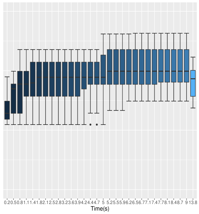
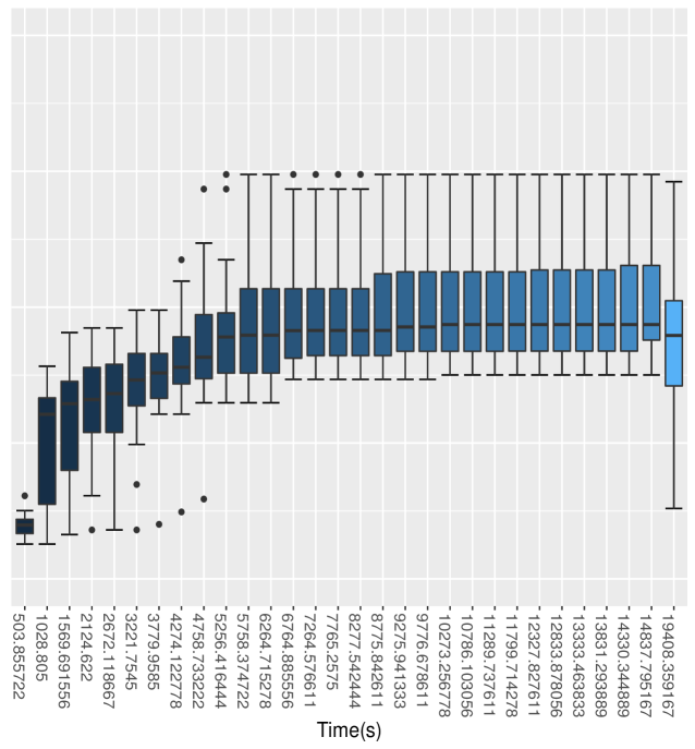
For all comparisons, we used independent runs of each method and present the average results from these runs. To show the variation in runs, we present box-plots of efficiency in relation to computation time from the runs of Nested Adaptation. The final (right-most) box-plot in each such figures shows the final efficiency estimates from larger runs. Not surprisingly, these can be lower than obtained by shorter runs. These final estimates are reported in the tables.
A public Github repository containing scripts for reproducing our results may be found at https://github.com/nxdao2000/AutoAdaptMCMC. Some additional experiments are also provided there.
4.1 Linear state space model
First, to illustrate the distinction between the Nested Adaptation algorithm and other methods, we will use a linear state space model (Durbin and Koopman, 2012) in which all parameters are fixed. Such a model will allow us to provide a simple assessment of the performances of the methods for a range of situations, including those in which the models were true.
Let be the latent state at time , be the observed data, and suppose we have the number of time points . Let the initial priors be:
and observation density for State transitions are governed by a first order autoregressive (AR) process
| Algorithms | Adapt time | Efficiency | Time to effective samples |
|---|---|---|---|
| All Blocked | 0.00 | 52.359 | 1910 |
| Default | 0.00 | 1198.128 | 83 |
| All Scalar | 0.00 | 1218.060 | 82 |
| Auto Block | 22.92 | 1277.639 | 101 |
| Nested Adaptation 5K | 0.9 | 1796.079 | 56 |
| Nested Adaptation 10K | 1.7 | 1693.929 | 61 |
| Nested Adaptation 20K | 3.3 | 1616.752 | 65 |

and were randomly generated from simulating , with while and are subsequently generated using transition density with the parameter values and . These values were arbitrarily chosen to cover the range observed for the explanatory variables; we desire high efficiency regardless of model fit, so the particular choice of this simple model is tangential to our main points.
In this relatively simple example, we try our Nested Adaptation algorithm with large numbers of iterations in each outer adaptation as well as a large number of iterations for the final efficiency. Specifically, we used samples sizes of 5000, 10000 and 20000 per outer adaptation and we used for computing final efficiency.
For this example (Table 1) All Scalar sampling produces MCMC efficiency of about , while the All Blocked algorithm, which consists of a single block sampler of dimension , has MCMC efficiency of approximately . All Blocked samples all dimensions jointly, which requires computation time roughly double that of All Scalar and yields only rather low ESS. The Default algorithm performs similarly to Auto Block but worse than Nested Adaptation algorithm. Since Auto Block converges to All Scalar in this case, the Auto Block algorithm performs no better than standard All Scalar (Figure 1) as would be expected. It is clear that Nested Adaptation method has dramatic improvements even when we take into account the adaptation time. Amongst these Auto methods, Auto Block performs worse than all Nested Adaptation 5K, Nested Adaptation 10K and Nested Adaptation 20K in both computational time and MCMC efficiencies. Overall, Nested Adaptation 5K appears to be the most efficient method in terms of time to 10000 effective samples. One interpretation is that Nested Adaptation 5K trades off well between adaptation time and MCMC efficiency in this model. The final samplers from Nested Adaptation included an automated factor slice sampler on block (a, b), an automated factor random walk sampler on block (, ) and adaptive random-walk Metropolis-Hastings samplers on other nodes.
Figure 1 illustrates that Nested Adaptation algorithm outperforms the other algorithms. This comes from both the flexibility to trade-off the number of outer adaptations vs. adaptive time to reach a good sampler as well as the larger space of kernels being explored. Since MCMC efficiency is highly dependent upon hierarchical model structures, using scalar and multivariate normal random walks alone, as done by the Auto Block algorithm, can be quite limiting. Nested Adaptation, can overcome this limitation with the flexibility to choose different type of samplers. We will see that more strongly in the next examples, where the models are more complex.
4.2 A random effect model
We consider the “litters” model, which is an original example model provided with the MCMC package WinBUGS. This model is chosen because of its notoriously slow mixing, which is due to the strong correlation between parameter pairs. It is desirable to show how much improvement can be achieved compared to other approaches on this benchmark example. The purpose of using this simple example is to establish the potential utility of the Nested Adaptation approach, while saving more advanced applications for future work. In this case, we show that our algorithm indeed outperforms by a significant margin the other approaches. This model’s specification is given following Deely and Lindley (1981) and Kass and Steffey (1989) as follows.
| Algorithms | Adapt time | Efficiency | Time to effective samples |
|---|---|---|---|
| All Blocked | 0.00 | 0.5855 | 17079 |
| Default | 0.00 | 1.8385 | 5439 |
| All Scalar | 0.00 | 1.6870 | 5928 |
| Auto Block | 21.97 | 12.1205 | 847 |
| Nested Adaptation 50K | 4.09 | 16.4532 | 612 |
| Nested Adaptation 70K | 5.95 | 18.0358 | 560 |
| Nested Adaptation 100K | 8.34 | 17.6278 | 576 |
Suppose we observe the data in groups. In each group, the data , are conditionally independent given the parameters , with the observation density
In addition, assume that for fixed are conditionally independent given the “hyper-parameters” , , with conjugate density
Assume that , follow prior densities,
Following the setup of Rue and Held (2005) as discussed in Turek et al. (2017), we could jointly sample the top-level parameters and conjugate latent states as the beta-binomial conjugacy relationships allow the use of what Turek et al. (2017) call cross-level sampling, but, for demonstration purposes, we do not include this here.
Since the litters model mixes poorly, we run a large number of iterations (i.e. ) to produce stable estimates of final MCMC efficiency. We start both Auto Block and Auto Adapt algorithms with All Scalar and adaptively explore the space of all given candidate samplers. We use Nested Adaptation with either 50000, 70000 or 100000 iterations per outer adaptation.
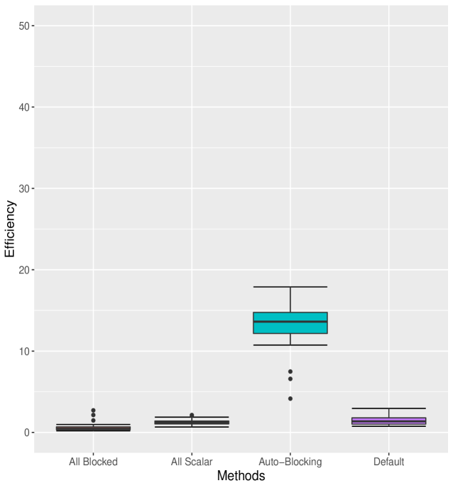
Results (Table 2) show that Auto Block generates samples with MCMC efficiency about seven-fold, six-fold and twenty-fold that of the All Scalar, Default and All Blocked methods, respectively. We can also see that as the outer adaptation sample size increases, the performance of Nested Adaptation improves. Final MCMC efficiencies of Nested Adaptation 50K, Nested Adaptation 70K and Nested Adaptation 100K are 135%, 148% and 145% of MCMC efficiency of Auto Block, respectively. In addition, the adaptation time for all cases of Nested Adaptation are much shorter than for Auto Block. Combining adaptation time and final efficiency into the resulting time to 10000 effective samples, we see that in this case, larger samples in each outer iteration are worth their computational cost. In this example, the final samplers from Nested Adaptation included automated factor random walk samplers on blocks (, ) and (, ), a slice sampler on and adaptive Metropolis-Hastings samplers on all other nodes
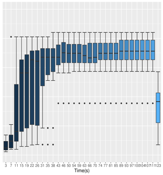
Figure 2 shows the box-plots computed from 20 independent runs on the litters model of All Blocked, All Scalar, Auto Block, Default and Nested Adaptation 50K algorithms. The left panel of the figure confirms that MCMC efficiency of Auto Block is well dominated that of other static adaptive algorithms. The right panel of the figure shows the MCMC efficiency of Nested Adaptation 50K gradually improves with time. The right-most box-plot verifies that the MCMC efficiency of selected samplers from Nested Adaptation algorithm (computed from large samples) is better than that of Auto Block algorithm. Last but not least, Nested Adaptation algorithms are much more efficient than Auto Block in the sense that we can keep every sample while Auto Block algorithm throws away most of the samples.
4.3 Spatial model
In this section, we consider a hierarchical spatial model as the final example. We use the classical scallops dataset for this model. This dataset is chosen since we want to compare our approach with other standard approaches in the presence of spatial dependence. This data collects observations of scallop abundance at 148 locations from the New York to New Jersey coastline in 1993. It was surveyed by the Northeast Fisheries Science Center of the National Marine Fisheries Service and made publicly available at http://www.biostat.umn.edu/~brad/data/myscallops.txt. It has been analyzed many times, such as Ecker and Heltshe (1994); Ecker and Gelfand (1997); Banerjee et al. (2004) and references therein. Following Banerjee et al., assume the log-abundance follows a multivariate normal distribution with mean and covariance matrix , defined by covariances that decay exponentially as a function of distance. Specifically, let be measured scallop abundance at site , be the distance between sites and , and be a valid correlation. Then
where each component
We model observations as . Priors for and are Uniform over a large range of interest. The parameters in the posterior distribution are expected to be correlated as the covariance structure induces a trade-off between and . This can be sampled well by Auto Block algorithm, and we would like to show that our approach can achieve even higher efficiency with lower computational cost of adaptation.
This spatial model, with 858 parameters, is computationally expensive to estimate. Therefore, we will use Nested Adaptation 5K, Nested Adaptation 10K and Nested Adaptation 20K algorithms for comparison and run for estimating final efficiency. In this case, the typical final samplers from Nested Adaptation included an automated factor random walk sampler on block (, ), adaptive random walk samplers on blocks (, , , ) and (, ), an automated factor slice sampler on block (, , , , ), slice samplers on , , and , and adaptive random-walk Metropolis-Hastings samplers on the rest.
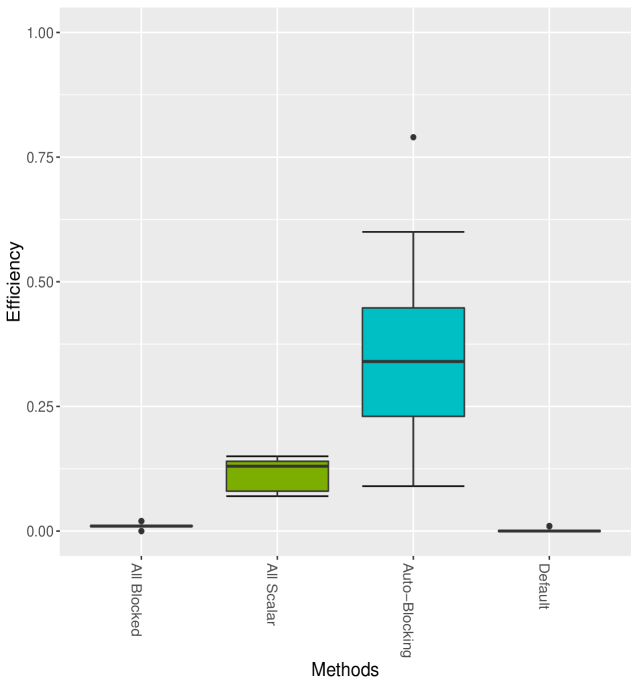
As can be seen from Table 3, All Blocked and Default algorithms mix very poorly, resulting in extremely low efficiencies of 0.01 and 0.002, respectively. The All Scalar algorithm, while achieving higher ESS, runs slowly because large matrix calculations are needed for every univariate sampler. The Auto Block algorithm, on the other hand, selects an optimal threshold to cut the entire hierarchical clustering tree into different groups, increasing the ESS about 3 times. With a few small blocks, the computation cost of Auto Block is somewhat cheaper than All Scalar algorithm. As a result, the efficiency mean is about 3.5 times that of All Scalar. Meanwhile, our Nested Adaptation 5K, 10K and 20K algorithms perform best. It should be noted that the Nested Adaptation algorithm can achieve good mixing with adaptation times that are only 15.5%, 32.5% and 59% compared to the adaptation time of Auto Block. In Figure 3, while the left panel shows a distinction between Auto Block and other static algorithms, the right panel shows that Nested Adaptation 20K surpasses Auto Block in just a few outer iterations, indicating substantial improvements in some models.
| Algorithms | Adapt time | Efficiency | Time to effective samples |
|---|---|---|---|
| All Blocked | 0.00 | 0.0100 | 1000000 |
| Default | 0.00 | 0.0020 | 5000000 |
| All Scalar | 0.00 | 0.1150 | 86956 |
| Auto Block | 19094.89 | 0.3565 | 47145 |
| Nested Adaptation 5K | 2967.55 | 0.4420 | 25592 |
| Nested Adaptation 10K | 6221.61 | 0.4565 | 28127 |
| Nested Adaptation 20K | 11278.78 | 0.4948 | 31488 |
5 Discussion
We have proposed a general Nested Adaptation MCMC algorithm. Our algorithm traverses a space of valid MCMC kernels to find an efficient algorithm automatically. There is only one previous approach, namely Auto Block sampling, of this kind that we are aware of. We have shown that our approach can substantially outperform Auto Block in some cases, and that both outperform simple static approaches. Using some benchmark models, we observe that our approach can yield improvements, which can be substantial compared to the Default method.
The comparisons presented have deliberately used fairly simple samplers as options for Nested Adaptation in order to avoid comparisons among vastly different computational implementations. A major feature of our framework is that it can incorporate almost any sampler as a candidate and almost any strategy for choosing new kernels from compositions of samplers based on results so far. Samplers to be explored in the future could include auxiliary variable algorithms such as slice sampling or derivative-based sampling algorithms such as Hamiltonian Monte Carlo (Duane et al., 1987). Now that the basic framework is established and shown to be useful in simple cases, it merits extension to more advanced cases.
The Nested Adaptation method can be viewed as a generalization of the Auto Block method. It is more general in the sense that it can use more kinds of samplers and explore the space of samplers more generally than the correlation-clustering of Auto Block. Thus, our framework can be considered to provide a broad class of automated kernel construction algorithms that use a wide range of sampling algorithm as components.
If block sampling is included in the space of the candidate samplers, choosing optimal blocks is important and can greatly increase the efficiency of the algorithm. For this reason, we extended the cutting of a hierarchical cluster tree to allow different cut heights on different branches (different parts of the model). This differs from Auto Block, which forms all blocks by cutting the entire tree at the same height. We also have different multivariate adaptive sampling other than random walk normal distribution such as automated factor slice sampler and automated factor random walk sampler. With these extensions, the final efficiency achieved by our algorithm specifically among blocking schemes is often substantially better and is found in a shorter time.
Beyond hierarchical clustering, there are other approaches one might consider to find efficient blocking schemes. One such approach would be to use the structure of the graph instead of posterior correlations to form blocks. This would allow conservation of calculations that are shared by some parts of the graph, whether or not they are correlated. Another future direction could be to improve how a new kernel is determined from previous results, essentially to determine an effective strategy for exploring the very high-dimensional kernel space. Finally, the trade-off between computational cost and the accuracy of effective sample size estimates is worth further exploration.
Development of Nested Adaptation MCMC has also raised several theoretical questions for future work. First, similarly to other adaptive MCMC methods, can more general conditions of validity be proven? Second, the estimation of effective sample size from a chain generated using Nested Adaptation is difficult because the properties of the kernel will have changed during the course of sampling. Methods for estimating effective sample size typically don’t consider such a situation. Third, what are good choices for the external and internal adaptation schedules (e.g. and in Section 2)? Fourth, how can we disentangle the contribution of each sampler to mixing achieved by a kernel comprising multiple samplers? Doing so could enable better moves in kernel space during outer adaptation. Finally, what are good strategies for parallelization of Nested Adaptation?
References
- Andrieu and Atchadé (2006) Andrieu, C. and Atchadé, Y. F. (2006). “On the efficiency of adaptive MCMC algorithms.” In Proceedings of the 1st International Conference on Performance Evaluation Methodolgies and Tools, 43. ACM.
- Andrieu and Moulines (2003) Andrieu, C. and Moulines, E. (2003). “Ergodicity of some adaptive Markov chain Monte Carlo algorithm.” Technical report.
- Andrieu and Robert (2001) Andrieu, C. and Robert, C. P. (2001). “Controlled MCMC for optimal sampling.” Preprint.
- Andrieu and Thoms (2008) Andrieu, C. and Thoms, J. (2008). “A tutorial on adaptive MCMC.” Statistics and Computing, 18(4): 343–373.
- Atchade and Fort (2010) Atchade, Y. and Fort, G. (2010). “Limit theorems for some adaptive MCMC algorithms with sub-geometric kernels.” Bernoulli, 16(1): 116–154.
- Atchadé et al. (2011) Atchadé, Y., Fort, G., Moulines, E., and Priouret, P. (2011). “Adaptive Markov chain Monte Carlo: theory and methods.” In Bayesian time series models, 32–51. Cambridge Univ. Press, Cambridge.
- Atchadé et al. (2005) Atchadé, Y. F., Rosenthal, J. S., et al. (2005). “On adaptive Markov chain Monte Carlo algorithms.” Bernoulli, 11(5): 815–828.
- Banerjee et al. (2004) Banerjee, S., Carlin, B. P., and Gelfand, A. E. (2004). Hierarchical Modeling and Analysis for Spatial Data. Chapman and Hall/CRC.
- de Valpine et al. (2017) de Valpine, P., Turek, D., Paciorek, C. J., Anderson-Bergman, C., Lang, D. T., and Bodik, R. (2017). “Programming with models: writing statistical algorithms for general model structures with NIMBLE.” Journal of Computational and Graphical Statistics, 26(2): 403–413.
- Deely and Lindley (1981) Deely, J. and Lindley, D. (1981). “Bayes empirical bayes.” Journal of the American Statistical Association, 76(376): 833–841.
- Duane et al. (1987) Duane, S., Kennedy, A. D., Pendleton, B. J., and Roweth, D. (1987). “Hybrid Monte Carlo.” Physics Letters B, 195(2): 216–222.
- Durbin and Koopman (2012) Durbin, J. and Koopman, S. J. (2012). Time Series Analysis by State Space Methods, volume 38. Oxford University Press.
- Ecker and Heltshe (1994) Ecker, M. and Heltshe, J. (1994). “Geostatistical estimates of scallop abundance.” Case Studies in Biometry, 107–124.
- Ecker and Gelfand (1997) Ecker, M. D. and Gelfand, A. E. (1997). “Bayesian variogram modeling for an isotropic spatial process.” Journal of Agricultural, Biological, and Environmental Statistics, 347–369.
- Everitt et al. (2011) Everitt, B. S., Landau, S., Leese, M., and Stahl, D. (2011). “Hierarchical clustering.” Cluster Analysis, 5th Edition, 71–110.
- Gilks et al. (1998) Gilks, W. R., Roberts, G. O., and Sahu, S. K. (1998). “Adaptive Markov chain Monte Carlo through regeneration.” Journal of the American Statistical Association, 93(443): 1045–1054.
- Guennebaud et al. (2010) Guennebaud, G., Jacob, B., et al. (2010). “Eigen.” URL: http://eigen. tuxfamily. org.
- Haario et al. (2001) Haario, H., Saksman, E., and Tamminen, J. (2001). “An adaptive Metropolis algorithm.” Bernoulli, 223–242.
- Haario et al. (2005) — (2005). “Component-wise adaptation for high dimensional MCMC.” Computational Statistics, 20(2): 265–273.
- Kass and Steffey (1989) Kass, R. E. and Steffey, D. (1989). “Approximate Bayesian inference in conditionally independent hierarchical models (parametric empirical Bayes models).” Journal of the American Statistical Association, 84(407): 717–726.
- Łatuszyński et al. (2013) Łatuszyński, K., Roberts, G. O., and Rosenthal, J. S. (2013). “Adaptive Gibbs samplers and related MCMC methods.” The Annals of Applied Probability, 23(1): 66–98.
- Lunn et al. (2012) Lunn, D., Jackson, C., Best, N., Thomas, A., and Spiegelhalter, D. (2012). The BUGS Book: A Practical Introduction to Bayesian Analysis. CRC Press.
- Lunn et al. (2000) Lunn, D. J., Thomas, A., Best, N., and Spiegelhalter, D. (2000). “WinBUGS-a Bayesian modelling framework: concepts, structure, and extensibility.” Statistics and Computing, 10(4): 325–337.
- Plummer et al. (2006) Plummer, M., Best, N., Cowles, K., and Vines, K. (2006). “CODA: convergence diagnosis and output analysis for MCMC.” R News, 6(1): 7–11.
-
R Core Team (2013)
R Core Team (2013).
“R: A Language and Environment for Statistical
Computing.”
URL http://www.R-project.org/ - Roberts and Rosenthal (2001) Roberts, G. O. and Rosenthal, J. S. (2001). “Optimal scaling for various Metropolis-Hastings algorithms.” Statistical Science, 16(4): 351–367.
- Roberts and Rosenthal (2007) — (2007). “Coupling and ergodicity of adaptive Markov chain Monte Carlo algorithms.” Journal of Applied Probability, 44(2): 458–475.
- Roberts and Rosenthal (2009) — (2009). “Examples of adaptive MCMC.” Journal of Computational and Graphical Statistics, 18(2): 349–367.
- Roberts et al. (1998) Roberts, G. O., Rosenthal, J. S., et al. (1998). “Two convergence properties of hybrid samplers.” The Annals of Applied Probability, 8(2): 397–407.
- Rue and Held (2005) Rue, H. and Held, L. (2005). Gaussian Markov Random Fields: Theory and Applications. CRC Press.
- Sahu et al. (2003) Sahu, S. K., Zhigljavsky, A. A., et al. (2003). “Self-regenerative Markov chain Monte Carlo with adaptation.” Bernoulli, 9(3): 395–422.
- Straatsma et al. (1986) Straatsma, T., Berendsen, H., and Stam, A. (1986). “Estimation of statistical errors in molecular simulation calculations.” Molecular Physics, 57(1): 89–95.
- Thompson (2010) Thompson, M. B. (2010). “Graphical comparison of MCMC performance.” arXiv preprint arXiv:1011.4457.
- Tibbits et al. (2014) Tibbits, M. M., Groendyke, C., Haran, M., and Liechty, J. C. (2014). “Automated factor slice sampling.” Journal of Computational and Graphical Statistics, 23(2): 543–563.
- Turek et al. (2017) Turek, D., de Valpine, P., Paciorek, C. J., and Anderson-Bergman, C. (2017). “Automated parameter blocking for efficient Markov chain Monte Carlo sampling.” Bayesian Analysis, 12(2): 465–490.
This work was funded in part by a grant from the U.S. National Science Foundation SI2-SSI program (ACI-1550488).
Appendix A Block MCMC sampling
This section provides the validity of block sampling in our general framework. We apply the results of Łatuszyński et al. (2013) for block Gibbs samplers. Following closely their notation, let be an -dimensional state space where , so that the total dimension is . We write as and set so that
For , let the conditional distribution of . We now consider a class of adaptive block MCMC sampler algorithms as follows.
ALGORITHM of Nested Adaptation Block MCMC.
(1) Set where is an outer adaptation function to select in .
(2) Choose block in that order.
(3) Draw where is a proposal distribution.
(4) Set
where
To establish the results for Nested Adaptation Block MCMC, we need the following assumption.
Assumption A.1.
For every and , the transition kernel is uniformly ergodic. Moreover, there exist and an integer s.t. for every and , there exists a probability measure on , s.t. for every .
We have the following results, similar to Theorem 4.19 of Łatuszyński et al. (2013).
Theorem A.1.
Assume that Assumption A.1 holds. Then Nested Adaptation Block MCMC is ergodic. That is, as . Moreover, if
in probability, then convergence of Nested Adaptation Block MCMC is also uniform over all that is,
as .
Proof.
To prove, we check simultaneous uniform ergodicity and the diminishing adaptation property of the algorithm and apply the result from Theorem 1 of Roberts and Rosenthal (2007) to conclude. We proceed as in the proof of Łatuszyński et al. (2013), Theorem 4.10 to establish simultaneous uniform ergodicity. By Assumption 1 and Lemma 4.14 of Łatuszyński et al. (2013), every adaptive Metropolis transition kernel for the block, , has stationary distribution and is -strongly uniformly ergodic. Since each block is sampled at least once by our construction and there is only a finite dimension, the probability of selecting each block is positive and bounded away from . In other word, there exists such that . Observe also that the family of block MCMC , is -strongly uniformly ergodic for some by Łatuszyński et al. (2013) Lemma 4.15. Hence, the family of adaptive block Metropolis-within-Gibbs samplers indexed by , is -simultaneously strongly uniformly ergodic with some and given as in (Roberts et al., 1998). Therefore we have that simultaneous uniform ergodicity is satisfied. Diminishing adaptation follows from Proposition 1 and from our construction. Therefore we can conclude the result. ∎