Network-Aware Optimization of
Distributed Learning for Fog Computing
Abstract
Fog computing promises to enable machine learning tasks to scale to large amounts of data by distributing processing across connected devices. Two key challenges to achieving this goal are (i) heterogeneity in devices’ compute resources and (ii) topology constraints on which devices communicate with each other. We address these challenges by developing a novel network-aware distributed learning methodology where devices optimally share local data processing and send their learnt parameters to a server for periodic aggregation. Unlike traditional federated learning, our method enables devices to offload their data processing tasks to each other, with these decisions optimized to trade off costs associated with data processing, offloading, and discarding. We analytically characterize the optimal data transfer solution under different assumptions on the fog network scenario, showing for example that the value of offloading is approximately linear in the range of computing costs in the network when the cost of discarding is modeled as decreasing linearly in the amount of data processed at each node. Our experiments on real-world data traces from our testbed confirm that our algorithms improve network resource utilization substantially without sacrificing the accuracy of the learned model, for varying distributions of data across devices. We also investigate the effect of network dynamics on model learning and resource costs.
Index Terms:
federated learning, offloading, fog computingI Introduction
New technologies like autonomous cars and smart factories are coming to rely extensively on data-driven machine learning (ML) algorithms [2, 3, 4] to produce near real-time insights based on historical data. Training ML models at realistic scales, however, is challenging, given the enormous computing power required to process today’s data volumes. The collected data is also dispersed across networks of devices, while ML models are traditionally managed in a centralized manner [5].
Fortunately, the rise in data generation in networks has occurred alongside a rise in the computing power of networked devices. Thus, a possible solution for real-time training of and inferencing from data-driven ML algorithms lies in the emerging paradigm of fog computing, which aims to design systems, architectures, and algorithms that leverage device capabilities between the network edge and cloud [6]. Deployment of 5G wireless networks and the Internet of Things (IoT) is accelerating adoption of this computing paradigm by expanding the set of connected devices with compute capabilities and enabling direct device-to-device communications between them [7]. Though centralized ML algorithms are not optimized for such environments, distributed data analytics is expected to be a major driver of 5G adoption [8].
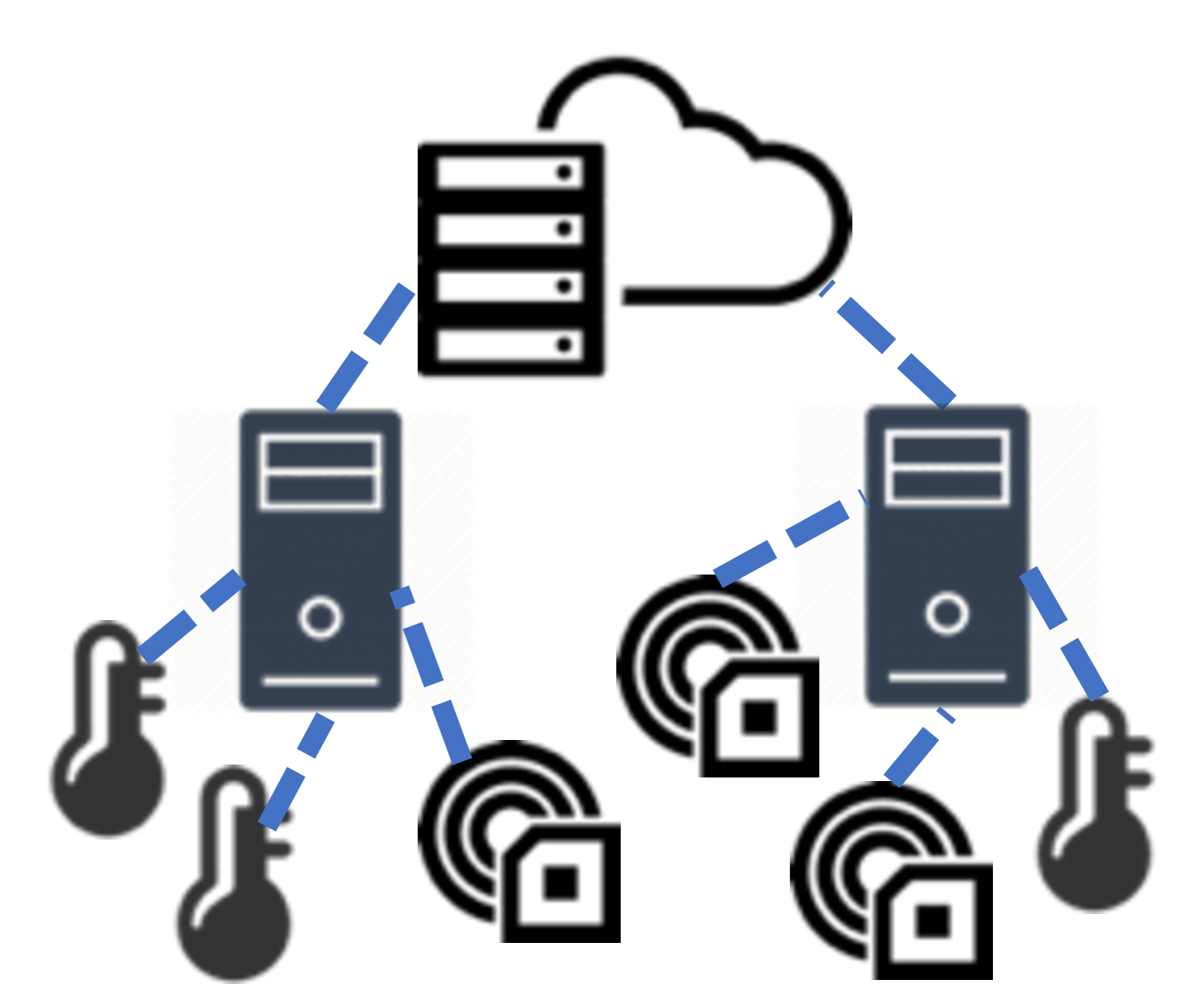
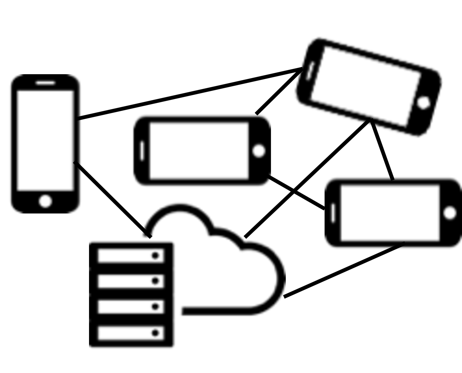
Initial efforts in decentralizing ML have focused on decomposing model parameter updates over several nodes, typically managed by some centralized server [9, 10]. Most of these methods implicitly assume idealized network topologies where node and link properties are homogeneous. Fog environments, by contrast, are characterized by devices’ computation and communication resource heterogeneity, e.g., due to power constraints or privacy considerations. For example, consider the two common fog topologies depicted in Figure 1. In the hierarchical scenario, weaker edge devices are connected to powerful edge servers. In the social network case, devices tend to have similar compute resources, but connectivity may vary significantly depending on levels of trust between users [11].
A central question that arises, then, in adapting ML methodologies to fog environments is: How should each fog device contribute to the ML training and inference? The examples above motivate techniques for network-aware distributed learning, which (i) account for the potentially heterogeneous computation and communication resources across devices, and (ii) leverage the network topology for device communications to optimize the distribution of data processing through the network. In this paper, we develop a novel network-aware distributed learning methodology that optimizes the distribution of processing across a network of fog devices.
I-A Machine Learning in Fog Environments
ML models are generally trained by iteratively updating estimates of parameter values, such as weights in a neural network, that best “fit” empirical data, through data processing at one or more devices. We face two major challenges in adapting such training to fog networking environments: (i) heterogeneity in devices’ compute resources and (ii) constraints on devices’ abilities to communicate with each other. We outline these characteristics, and the potential benefits enabled by our network-aware distributed learning methodology, in some key applications below:
Privacy-sensitive applications. Many ML applications learn models on sensitive user data, e.g., for health monitoring [4]. Due to privacy concerns, most of these applications have devices train their models on local data to avoid revealing data to untrustworthy nodes [11]. Offloading ML data processing to trusted devices, e.g. if one user owns multiple devices, can reduce training times and improve model accuracy.
Internet-connected vehicles can collaboratively learn about their environment [2], e.g., by combining their data with that of road sensors to infer current road or traffic conditions. Since sensors have less computing capabilities than vehicles, they will likely offload their data to vehicles or roadside units for processing. This offloading must adapt as vehicles move and their connectivity with (stationary) road sensors changes.
Augmented reality (AR) uses ML algorithms for e.g., image recognition [3] to overlay digital content onto users’ views of an environment. A network of AR-enabled devices can distributedly train ML models, but may exhibit significant heterogeneity: they can range from generic smartphones to AR-specific headsets, with different battery levels. As the AR users move, connectivity between devices will also change.
Industrial IoT. 5G networks will allow sensors that power control loops in factory production lines to communicate across the factory floor [2, 12], enabling distributed ML algorithms to use this data for, e.g., predicting production delays. Determining which controllers should process data at specific sensors is an open-question: it depends on sensor-controller connectivities, which may vary with factory activity.
I-B Outline and Summary of Contributions
First, Section II differentiates our work from relevant literature. To the best of our knowledge, we are the first to optimize the distribution of ML data processing (i.e., training) tasks across fog nodes, leading to several contributions:
Formulating the task distribution problem (Section III). In deciding which devices should process which datapoints, our formulation accounts for resource limitations and model accuracy. While ideally more of the data would be processed at devices with more computing resources, sending data samples to such devices may overburden the network. Moreover, processing too many data samples can incur large processing costs relative to the gain in model accuracy. We derive new bounds (Theorem 1) on the model accuracy when data can be moved between devices, showing that the optimal task distribution problem can be formulated as a convex optimization.
Characterizing the optimal task distribution (Section IV). Solving the optimization in Sec. III requires specifying network characteristics that may be unknown in advance. We analyze the expected deviations from our assumptions in Sec. III to derive guidelines on estimating these characteristics (Theorem 2). We then consider two different models of discard cost, one linear and one convex in the number of datapoints processed, and use them to derive the optimal distribution of data processing through the network for typical fog topologies (Theorems 3 and 4). Further, we use the result from the linear case to estimate the reduction in processing costs due to data movement (Theorem 5). Overall, these results are the first to characterize the integration of offloading into federated learning over graph topologies.
Experimental validation (Section V). We train classification models on the MNIST dataset to validate our algorithms. We use a Raspberry Pi testbed to emulate network delays and available compute resources, under both i.i.d. and non-i.i.d. device data. Our proposed algorithm nearly halves the processing overhead yet achieves an accuracy comparable to centralized model training, which validates the benefits of network-aware distributed learning. The experiments also reveal how the network connectivity, size, and topology structure impact the trained model accuracy and network resource costs.
II Related Work
We contextualize our work within prior results on (i) federated and distributed machine learning, and (ii) methods for offloading ML tasks from mobile devices to edge servers.
II-A Distributed and Federated Learning
In classical distributed learning, “workers” each compute a parameter value from their local data. These results are aggregated at a central server, and updated parameter values are sent to the workers for the next round of local computations. Several works have considered how network topologies can affect ML training. Specifically, [13] optimizes decentralized training of linear models when workers exchange parameters with their neighbors instead of a central server, while [14] studied D2D (device-to-device) message passing that emulates global communications with a server, and [15] optimizes performance when communications can fail. In fog networks, devices may not have the resources to send updates to a server at every time period [5], so we focus on the newer federated learning methodology for distributed model training.
Devices in federated learning perform a series of local updates between aggregations, and send their resulting model updates to the server [16, 17, 10]. This framework preserves user privacy by keeping data at local devices [18] and reduces the amount of communication between devices and the central server. Since its proposition in [10], federated learning has generated significant research interest; see [19] for a comprehensive survey. Compared to traditional distributed learning, federated learning introduces two new challenges: firstly, data may not be identically and independently distributed as devices locally generate the samples they process; and secondly, in fog/edge networks, devices may have limited ability to perform and communicate local updates due to resource constraints. Many works have attempted to address the first challenge; for instance, [20] trains user-specific models within a multi-task learning framework, while [21] showed that sharing small subsets of user data can significantly increase the accuracy of a single model. Recent efforts have also considered optimizing the frequency of parameter aggregations according to a fixed budget of network and computing resources [5], or adopting a peer-to-peer decentralized learning framework [22].
Our work is more related to the second challenge of resource heterogeneity. Existing works have focused on minimizing the communication costs between the workers and the server. Specifically, [23] proposes to reduce uplink costs by restricting and compressing the parameter space prior to transmission. [24] proposes a method for thresholding updates for transmission, while the method in [25] only communicates the most important individual gradient results, which [26] extends to compress both downlink and uplink communication. To reduce the number of uplink transfers, [27, 28] aggregate subsets of the network. For wireless networks in particular, [29] proposes methods to minimize power consumption and training time.
Unlike these works, we focus on the network topology between nodes to optimize the tradeoffs among communication, computation, and model performance in federated learning. Specifically, our work leverages D2D communications for offloading data from resource-constrained to resource-rich nodes, as is present in new 5G and IoT network technologies [6]. In integrating D2D offloading with federated learning, we derive novel results on optimizing the distribution of data processing over a fog computing system to train ML models.
II-B Offloading
Fog computing introduces opportunities to pool network resources and maximize the use of idle computing/storage in completing resource-intensive activities [6]. Offloading mechanisms improve system performance when high-bandwidth network connections are available between devices. Offloading has significantly accelerated ML tasks such as linear regression training [30] and neural network inference [31]. Existing literature has also considered splitting different layers in deep neural networks between fog devices and edge/cloud servers. Specifically, [32] proposed two network-dependent schemes and a min-cut problem to accelerate the training phase, while [33] developed an architecture to intelligently locate models on local devices or the cloud based on network reliability.
Prior works on deep learning offloading in fog/edge computing generally focus on network factors, such as cost/latency, rather than model accuracy. For example, [34, 35] maximize throughput in wireless and sensor IoT networks. [36] studies D2D data offloading in federated learning, but focuses on communication protocols to facilitate over-the-air parameter aggregations and dataset duplication across nodes. Our methodology considers more general ML models, optimizes tradeoffs between network cost and model accuracy, and provides novel theoretical performance bounds.
III Model and Optimization Formulation
We first define our model for fog networks (Section III-A) and machine learning training (Section III-B), and then formulate the task distribution optimization problem (Section III-C).
III-A Fog Computing System Model
We consider a set of fog devices forming a network, an aggregation server , and discrete time intervals as the period for training an ML model. Each device, e.g., a sensor or smartphone, can both collect data and process it to contribute to the ML task. The server aggregates the results of each device’s local analysis, as will be explained in Section III-B. Both the length and number of time intervals may depend on the specific ML application. In each interval , we suppose a subset of devices , indexed by , is active (i.e., available to collect and/or process data). For simplicity of notation, we omit ’s dependence on .
III-A1 Data collection and processing
We use to denote the set of data collected by device for the ML task at time ; denotes each datapoint. Note, if a device does not collect data at time . , by contrast, denotes the set of datapoints processed by each device at time , for the ML task. In conventional distributed learning frameworks, , as all devices process the data they collect [5]; separating these variables is one of our main contributions. We suppose that each device can process up to datapoints at each time , incurring a cost of for each point. For example, devices with low battery will have lower capacities and higher costs .
III-A2 Fog network connectivity
The devices are connected to each other via a set of directed links between devices and ; denotes the set of functioning links at time . The overall system can then be described as a directed graph with vertices representing the devices and edges the links between them. We suppose that is connected at each time and that links between devices are single-hop, i.e., devices do not use each other as relays except possibly to communicate with the server. The scenarios outlined in Section I-A each possess such an architecture: in smart factories, for example, a subset of the floor sensors connect to each controller. Each link is characterized by a capacity , i.e., the maximum datapoints transferable in a time interval, and a per-unit “cost of connectivity” . This cost may reflect network conditions or a desire for privacy, and will be high if sending from to is less desirable at .
III-A3 Data structure
Each datapoint takes the form , where is an attribute/feature vector and is an associated label.111For unsupervised ML tasks, there are no labels . However, we can still minimize a loss defined in terms of the , similar to (1). We use to denote the full set of datapoints collected by all devices over all time. Following prior work [37, 38], we model data collection as each device sampling points uniformly at random from a (usually unknown) distribution . Temporal changes in are assumed to be slow compared to the time horizon . We use to denote the global distribution induced by these . Our model implies that the relationship between and is temporally invariant, which is common in the applications discussed in Section I-A, e.g., image recognition from road cameras at fixed locations or AR users with random mobility patterns. We use such a dataset for evaluation in Section V.
III-B Machine Learning Model
Our goal is to learn a parameterized model that outputs given the input feature vector . We use the vector to denote the set of model parameters, whose values are chosen so as to minimize a loss function that is defined for the specific ML model (e.g., squared error for linear regression, cross-entropy loss for multi-class classifiers [39]). Since the overall distributions are unknown, instead of minimizing we minimize the empirical loss function, as commonly done in ML model training (e.g., [5], [10]):
| (1) |
where is the error for datapoint , and is the number of datapoints. Note that the function may include regularization terms that aim to prevent model overfitting [10].
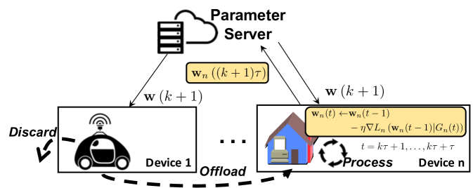
Fog computing allows (1) to be solved in a distributed manner: instead of computing the solution at the server , we can leverage computations at any device with available resources. Below, we follow the commonly used federated averaging framework [5] in specifying these local computations and the subsequent global aggregation by the server in each iteration, illustrated by device in Figure 2. To avoid excessive re-optimization at each device, the local updating algorithm does not depend on . We adjust the server averaging to account for the amount of data each device processes.
III-B1 Local loss minimization
To distributedly solve (1), we first decompose it into a weighted sum of local loss functions
| (2) |
where denotes the set of datapoints processed by device over all times. The global loss (1) is then if , i.e., all datapoints are eventually processed.
Loss functions such as (2) are typically minimized using gradient descent techniques [10]. Specifically, the devices update their local parameter estimates at according to
| (3) |
where is the step size or learning rate, and is the gradient with respect to of the average loss of points in the current dataset at the parameter value . We define the loss only on since future data in has not yet been revealed; since we assume each node’s data is i.i.d. over time, approximates the local loss . The computational cost of processing datapoint is then the cost of computing the gradient . If the local data distributions are all the same, then all datapoints are i.i.d. samples of this distribution, and this process is similar to stochastic gradient descent with batch size .
III-B2 Aggregation and synchronization
The aggregation server will periodically receive the local estimates from the devices, compute a global update based on these models, and synchronize the devices with the global update. Formally, the th aggregation is computed as
| (4) |
where is the fixed aggregation period and is the number of datapoints node processed since the last aggregation. Thus, the update is a weighted average factoring in the sample size on which each is based. Intuitively, since the objective in (1) minimizes the empirical loss [5, 10], nodes that process more data should be weighted more, as in (1)-(4).
III-C Optimization Model for Data Processing Tasks
We now consider the choice of , which defines the data processing task executed by device at time . There are two possible reasons : first, device may offload some of its collected data to another device or vice versa, e.g., if has insufficient capacity to process all of the data 222For notational convenience, here refers to the number of datapoints , and similarly refers to . The context will make the distinction clear throughout the paper. or if has lower computing costs . Second, device may discard data if processing it does not reduce the empirical loss (1) by much. In Figure 2, device 1 offloads or discards all of its data. We collectively refer to discarding and offloading as data movement.
III-C1 Data movement model
We define as the fraction of data collected at device that is offloaded to device at time . Thus, at time , device offloads amount of data to . Similarly, will denote the fraction of data collected at time that device also processes at time . We suppose that as long as , the capacity of the link between and , then all offloaded data will reach within one time interval and can be processed at device in time interval . Since devices must have a link between them to offload data, if .
We also define as the fraction of data collected by device at time that will be discarded. In doing so, we assume that device will not discard data that has been offloaded to it by others, since that has already incurred an offloading cost . The amount of data collected by device at time and discarded is then , and the amount of data processed by each device at time is
In defining the variables and , we have implicitly specified the constraint : all data collected by device at time must either be processed by device at this time, offloaded to another device , or discarded. We assume that devices will not store data for future processing, which would add another cost component to the model.
To quantify the cost of discarding relative to processing/offloading, we also define as the cost per unit model loss . The dependence on can capture the fact that certain devices in the network may weight their model error costs differently depending on the importance of the application. The dependence on can capture the fact that the loss may become less important relative to the resource utilization as the model approaches convergence.
III-C2 Data movement optimization
We formulate the following cost minimization problem for determining the data movement variables and over the time period :
| (5) | ||||
| subject to | (6) | |||
| (7) | ||||
| (8) | ||||
| (9) |
Constraints (6–8) were introduced above and ensure that the solution is feasible. The capacity constraints in (9) ensure that the amounts of data transferred and processed are within link and node capacities, respectively.
The three terms in the objective (5) correspond to the processing, offloading, and error costs, respectively. We do not include the cost of communicating parameter updates to/from the server in our model; unless a device processes no data, the number of updates stays constant. By including these three cost terms, our formulation accounts for the tradeoff between model performance and resource utilization:
(i) Processing, : This is the computing cost associated with processing of data at node at time .
(ii) Offloading, : This is the communication cost incurred from node offloading data to .
(iii) Error, : This cost quantifies the impact of data movement on the local model error at each device . As the model approaches convergence for large , improvement in the error term with respect to the variables becomes limited. Thus, we may have decrease over time to prioritize network costs at later time periods.
Since is computed as in (3), the model error term is an implicit function of . We include the error from each device ’s local model at each time , instead of considering the error of the final model, since devices may need to make use of their local models as they are updated (e.g., if aggregations are infrequent due to resource constraints [5]).
If the local datasets are i.i.d. (i.e., each is representative of the global distribution), then discarding more data clearly increases the global loss, since less data is used to train the ML model. Offloading may also skew the local model if it is updated over a small . We can, however, upper bound the loss function regardless of the data movement:
Theorem 1 (Upper bound on local loss).
If is convex, -Lipschitz, and -smooth, if , and if for a lower bound , then, after aggregations at time with a period and defining the constant , the local loss will satisfy
| (10) |
where , which implies is decreasing in , and is given by
Proof:
The full proof is contained in Appendix A of the supplementary material. We define , as the parameters under centralized gradient descent updates, , and assume as in [5]. After lower-bounding and , we can upper-bound as
Then, we let be the positive root of . The result follows since either or ; both imply (10). ∎
In Section IV, we will consider how to use Theorem 1’s result to find tractable forms of the loss expression that allow us to solve the optimization (5–9) efficiently. Moreover, without perfect information on the device costs, capacities, and error statistics over the time period , we cannot solve (5–9) exactly, so we will propose methods for estimating them.
IV Optimization Model Analysis
We turn now to a theoretical analysis of the data movement optimization problem (5)–(9). We discuss the choice of error cost and capacity values (Section IV-A), and then characterize the optimal solution under different choices of the error cost and assumptions on the fog networking scenario for the ML use cases outlined in Section I (Section IV-B).
IV-A Choosing Costs and Capacities
We may not be able to reliably estimate the costs , , and or capacities and in real time. Misestimations are likely in highly dynamic scenarios that use mobile devices, since the costs of offloading data depend on network conditions at the current device locations. Mobile devices are also prone to occasional processing delays called “straggler effects” [22], which can be modeled as variations in their capacities. The error cost, on the other hand, decreases over time as the model parameters move towards convergence. Here, we propose and analyze network characteristic selection methods. Although these methods also rely on some knowledge of the system, we show in Section V that a simple time-averaging of historical costs and capacities suffices to obtain reasonable data movement solutions.
IV-A1 Choosing capacities
Overestimating leads to the deferral of some data processing until future time periods, which may cause a cascade of processing delays. Misestimations of the link capacities have similar effects. Here, to limit delays due to overestimation, we formalize guidelines for the capacities in (9)’s constraints. As commonly done [40], we assume that processing times on stragglers follow an exponential distribution for parameter .
For device capacities, we obtain the following result:
Theorem 2 (Processing time with compute stragglers).
Suppose that the service time of processing a datapoint at node follows , and that , , are time invariant. We can ensure the average waiting time of a datapoint to be processed is lower than a given threshold by setting the device capacity such that , where is the smallest solution to the equation , an increasing function of .
Proof:
We note that the processing at node follows a D/M/1 queue with arrival rate , and the result follows from the average waiting time in such a queue. Details are in Appendix B of the supplementary material. ∎
For instance, guarantees an average processing time of less than one time slot, as assumed in Section III’s model. Thus, Theorem 2 shows that we can still (probabilistically) bound the data processing time when stragglers are present. As long as , where is defined based on any values of and , Theorem 2 holds for any data offloading and discarding policy, including the one provided by the solution to our optimization (5)-(9).
Network link congestion encountered in transferring data may also delay its processing, which can be handled by choosing the network capacity analogously to Theorem 2.
IV-A2 Choosing error expressions
To solve the optimization (5)–(9), we also need an expression of the error objective in terms of our decision variables. As shown in Theorem 1, we can bound the local loss at time in terms of a gradient divergence constant . The following in turn provides an upper bound for in terms of :
Lemma 1 (Error convergence).
Suppose the data distributions have finite second and third moments. Then there exists a constant independent of such that
| (11) |
where , , and is the total number of datapoints generated.
Proof:
We can express as the sum of , , and . We bound above by using the central limit theorem. Since is the average of , , we can view as samples from a distribution whose expected value is . We repeat this argument for . ∎
The bound in Lemma 1 is likely to be a loose bound for non-i.i.d data, since, with data movement, the resulting distribution of data at device will be a mixture of the original distributions at each device. The value of quantifies the degree to which local datasets are non-i.i.d. across devices. When the local datasets are i.i.d., and . Since we take the generated device datasets as given in the optimization, is independent of our decision variables and , and thus independent of . As a result, only the term from (11) is dependent on our decision variables. By substituting Lemma 1 into in Theorem 1, we see that . Since the other time-dependent terms in can be absorbed into , one choice of the error cost in (5) is , capturing diminishing marginal returns in .
Since is a convex function of , with this choice of error cost, (5–9) becomes a convex optimization problem and can be solved relatively easily in theory. When the number of variables is large, however – e.g., if the number of devices with time periods, as could be the case in the applications discussed in Section I-A – standard interior point solvers will be prohibitively slow [41]. In such cases, we may wish to approximate the error term with a linear function and leverage faster linear optimization techniques, i.e., to take the error cost as so the error decreases when increases. This choice eliminates the diminishing marginal returns in . For learning tasks that are of a critical nature (e.g., object detection in smart vehicles [2]), this may actually be more desirable in order to prioritize the trained model accuracy. Ultimately, in practice, the desired relationship between the resource and error costs in the optimization depends on the particular application.
We can further express . Since these last two terms are linear functions of , they can alternatively be viewed as part of the transmission cost in (5). Specifically, if we redefine in the objective, we can treat the error cost as , which is equivalent to minimizing , i.e., a cost proportional to the amount of data discarded at node . The analytical results we present in Sec. IV-B will use this form.
We can quantify the difference imposed by the linear approximation by considering the Taylor expansion of , where represents the quantity of processed data, i.e., , at a device. Our linear approximation is equivalent to the first order Taylor approximation of , i.e. , with . Taylor’s theorem shows that the error in this first order expansion is proportional to for some , which is increasing in [42, 43]. Thus, the approximation will have a larger difference when devices are processing more data. Later in Sec. V-B, our experiments will show that there can be a practical advantage to modeling the discard cost as without modifying the .
IV-B Optimal Task Distributions
Given a set of costs and capacities for the optimization (5–9), we now characterize the optimal data movement solutions. We consider two formulations that admit closed-form solutions and elucidate the relationships between our costs and decision variables: (i) convex discard costs over a hierarchical, static topology (Theorem 4), and (ii) linear discard costs over a general, possibly dynamic topology (Theorem 3).
IV-B1 General and dynamic network topology
First, we consider the case of a general network topologies. In this case, we can derive a closed-form solution for the data processing variables under the linear error term :
Theorem 3 (Data movement with linear discard cost).
Suppose for each device , i.e., its compute capacity always exceeds the data it collects as well as any data offloaded to it by . Then, if the error cost is modeled as , the optimal and will each be or , with the following conditions for them being at node :
| (12) |
where .
Proof:
Since in (8), each datapoint in is either discarded, offloaded, or processed at . It is optimal to choose the option with least marginal cost. ∎
This theorem implies that with a linear discard cost, in the absence of resource constraints, all data will either be processed, offloaded to the lowest cost neighbor, or discarded. Additionally, Theorem 3 quantifies how the link costs affect the amount of data offloaded, allowing us to write the fraction of data offloaded by device as , which is if and otherwise. We later use this point in the proofs for Theorems 5 and 6.
Fog use cases. We next move to characterize solutions for specific fog use cases outlined in Section I. Table I summarizes the topologies of these four applications. Networks in smart factories have fairly static topologies, since they are deployed in controlled indoor settings. They also exhibit a hierarchical structure, with less powerful devices connected to more powerful ones in a tree-like manner with devices at the same level unable to communicate, as shown in Figure 1. Connected vehicles have a similar hierarchical structure, with sensors and vehicles connected to more powerful edge servers, but their architectures are more dynamic as vehicles are moving. Similarly, AR applications feature (possibly heterogeneous) mobile AR headsets connected to powerful edge servers. Applications that involve privacy-sensitive data may have very different, non-hierarchical topologies as the links between devices are based on trust, i.e., comfort in sharing private information. Since social relationships generally change slowly compared to ML model training, these topologies are relatively static.
While the connected vehicles and AR settings require the generic topology treatment from Theorem 3, we can derive additional results for static hierarchical and social topologies:
IV-B2 Static and hierarchical topologies
In hierarchical scenarios, more powerful edge servers will likely always have sufficient capacity to handle all offloaded data, and they will likely have lower computing costs when compared to other devices. If the cost of discarding is linear, then from Theorem 3, sensors offload their data to the edge servers, unless the cost of offloading exceeds the difference in computing costs. We show in Section V that the network cost can exceed the savings from offloading to more powerful devices; in such cases, devices process or discard their data instead.
| Use case | Topology | Dynamics |
|---|---|---|
| Smart factories [2] | Hierarchical | Fairly static |
| Connected vehicles [2] | Hierarchical | Rapid changes |
| Augmented reality [3] | Hierarchical, | Rapid changes |
| heterogeneous | possible | |
| Privacy-sensitive [4, 22] | Social network | Fairly static |
When the cost of discarding is nonlinear, the optimal solution is less intuitive: it may be optimal to discard data if the additional processing cost outweighs the expected error reduction. If we consider multiple heterogeneous devices with static processing costs and data generation rates, each connected to a more powerful edge server over the same wireless network (and thus assumed with the same connectivity costs), we can find a closed form solution to our original optimization:
Theorem 4 (Data movement with nonlinear error costs).
Suppose that devices with static processing costs and data generation rates can offload to an edge server, indexed as . Assume that there are no resource constraints, , the costs of transmitting to the server are identical and constant, and the discard cost is given by as in Lemma 1. Then, letting denote the fraction of data offloaded for node , for sufficiently large, the optimal amount of data discarded is
| (13) |
Given the optimal , an optimal solution for is given by
| (14) |
Proof:
The full proof is contained in Appendix C. There we note that in the hierarchical scenario, the cost objective (5) can be rewritten as . Taking the partial derivatives with respect to and , and noting that a large forces for each node gives the result. ∎
Intuitively, as the costs or increase, so should the amount of data discarded, as in Theorem 4. Theorem 4 also shows that data is neither fully discarded nor offloaded, in contrast with Theorem 3, implying that convex error bounds lead to a more balanced distribution of data across nodes in the network. We do not include resource constraints in Theorem 4 in order to focus on the effects of the compute and transmission costs , , and on the optimal solution. In practice, an edge server would have nearly unlimited capacity to process the datapoints generated by the devices, as it is much more powerful, and often has access to a more reliable power source, than typical mobile devices. Intuitively, including the capacities and on the devices and links would further increase the amount of data discarded.
IV-B3 Socially-defined topologies
When networks are larger and have more complex topologies, we extrapolate from Theorem 3’s characterization of device behaviors to understand data movement in the network as a whole. Specifically, we consider a social topology in which edges between devices are defined by willingness to share data (Figure 1(b)). In such cases, we assume as nodes either trust each other to share data or do not; nodes that do not trust each other simply will not have an edge between them. We can find the fraction of devices that offload data, which allows us to determine the cost savings from offloading, when the error cost is linear:
Theorem 5 (Value of offloading).
Suppose the fraction of devices with neighbors equals . For a social network following a scale-free topology, for example, for some constant and . Suppose and over all time, where is the uniform distribution between and and no discarding occurs.
Then the average cost savings, compared to no offloading, equals
| (15) |
Proof:
The full proof is contained in Appendix D of the supplementary materials. There, we use the result of Theorem 3 to find the probability that devices have lower processing cost neighbors, from which we can determine (15). ∎
Thus, the reduction in cost from enabling device offloading in such scenarios is approximately linear in : as the range of computing costs increases, there is greater benefit from offloading, since devices are more likely to find a neighbor with lower cost. The processing cost model may for instance represent device battery levels drawn uniformly at random from (full charge) to (low charge). The expected reduction from offloading, however, may be less than the average computing cost , as offloading data to another device does not entirely eliminate the computing cost. Note we can use a similar technique to analyze the scenario where is either nonzero or follows a given distribution; however, the expression for cost savings is then more complex due to the need to compare (drawn from ) with (drawn from a convolution of with the distribution of ). Similarly, we do not generalize Theorem 5’s results to a non-uniform distribution due to the complexity in writing a closed-form solution as in (15). However, we expect similar observations to hold, i.e., offloading becomes more beneficial as the cost range increases.
Next, we consider the case in which resource constraints are present, e.g., for less powerful edge devices. We find the expected devices that will have tight resource constraints:
Theorem 6 (Probability of resource constraint violation).
Let be the number of devices with neighbors, and for each device with neighbors, let be the probability that any one of its neighbors has neighbors. Also let denote the distribution of resource capacities, assumed to be i.i.d. across devices, and let be constant. Then if devices offload as in Theorem 3, the expected number of devices whose capacity constraints are violated is
| (16) |
with defined as the probability a device with neighbors offloads its data based on the conditions in Theorem 3.
Proof:
This follows from Theorem 3, and from obtaining an expression for the expected amount of processed data at a node with neighbors when offloading is enabled. ∎
Theorem 6 makes two assumptions: and resource capacities being i.i.d. across devices. The former assumption models a constant rate of data generation (e.g., from regular monitoring of user activity). If is stochastic (e.g., from event-driven sensor readings with random event sequences), we may generalize (16) by taking an additional expectation over . The latter assumption is reasonable if we have no information about specific devices in the network, but know a range of possible hardware specifications that determine the compute capacities. This is likely to occur when there are a large number of devices; as we explain below, such a scenario is precisely where Theorem 6 is most useful.
Theorem 6 allows us to quantify the complexity of solving the data movement optimization problem when resource constraints are in effect. We observe that it depends on not just the resource constraints, but also on the distribution of computing costs (through ), since these costs influence the probability devices will want to offload in the first place. Additionally, Theorem 6 provides a guide for the most efficient way to solve optimization (5)–(9). If the expected number of resource violations is low, then following the procedure in Theorem 3 will produce a near-optimal solution that violates only a few resource constraints. We can then ensure these constraints are satisfied with minimal adjustments to the solution, e.g., optimizing over only the and variables for the affected nodes and their neighbors while fixing all other optimization variables, or even increasing the until the capacity constraints are satisfied. While this solution will not be optimal, (12) can be implemented distributedly, if each device sends each of its neighbors (i) its processing cost and (ii) estimates of , e.g., channel conditions at the receiver. Thus, it is significantly more efficient than solving (5)–(9) via a generic linear solver. On the other hand, if (16) is large, then we should solve (5)–(9) using a generic optimizer.
V Experimental Evaluation
In this section, we experimentally evaluate our methodology. After discussing the setup in Sec.V-A, we investigate the performance of network-aware learning in Sec. V-B. Then, we examine the effects of network characteristics, structure, and dynamics on our methodology in Sec. V-C to V-E.
| Learning Methodology | Synthetic Costs | Testbed Costs | ||
|---|---|---|---|---|
| MLP | CNN | MLP | CNN | |
| Centralized | 92.00% | 98.00% | 92.00% | 98.00% |
| Federated (i.i.d.) | 90.82% | 96.62% | 90.82% | 96.62% |
| Federated (non-i.i.d.) | 84.00% | 96.10% | 84.00% | 96.10% |
| Network-aware (i.i.d.) | 88.63% | 95.89% | 89.70% | 96.03% |
| Network-aware (non-i.i.d.) | 83.20% | 92.31% | 85.47% | 92.62% |
V-A Experimental Setup
Machine learning task and models. We consider image recognition as our machine learning task, using the MNIST dataset [44], which contains 70K images of hand-written digits labeled 0-9, i.e., a 10-class classification problem. We use 60K images as the training dataset , and the remainder as our test set. The number of samples at node is modeled using a Poisson arrival process with mean . For i.i.d. scenarios, each device generates by sampling uniformly at random and without replacement from . For non-i.i.d. scenarios, each device is limited to a random selection of five of the 10 possible labels. Device then samples uniformly at random from this chosen subset of labels. Data distributions are i.i.d. unless stated otherwise. We train multilayer perceptrons (MLP) and convolutional neural networks (CNN) for image recognition on MNIST. We use cross entropy [45] as the loss function , and a constant learning rate . Unless otherwise stated, results are reported for CNN using fog devices, an aggregation period , and time intervals.
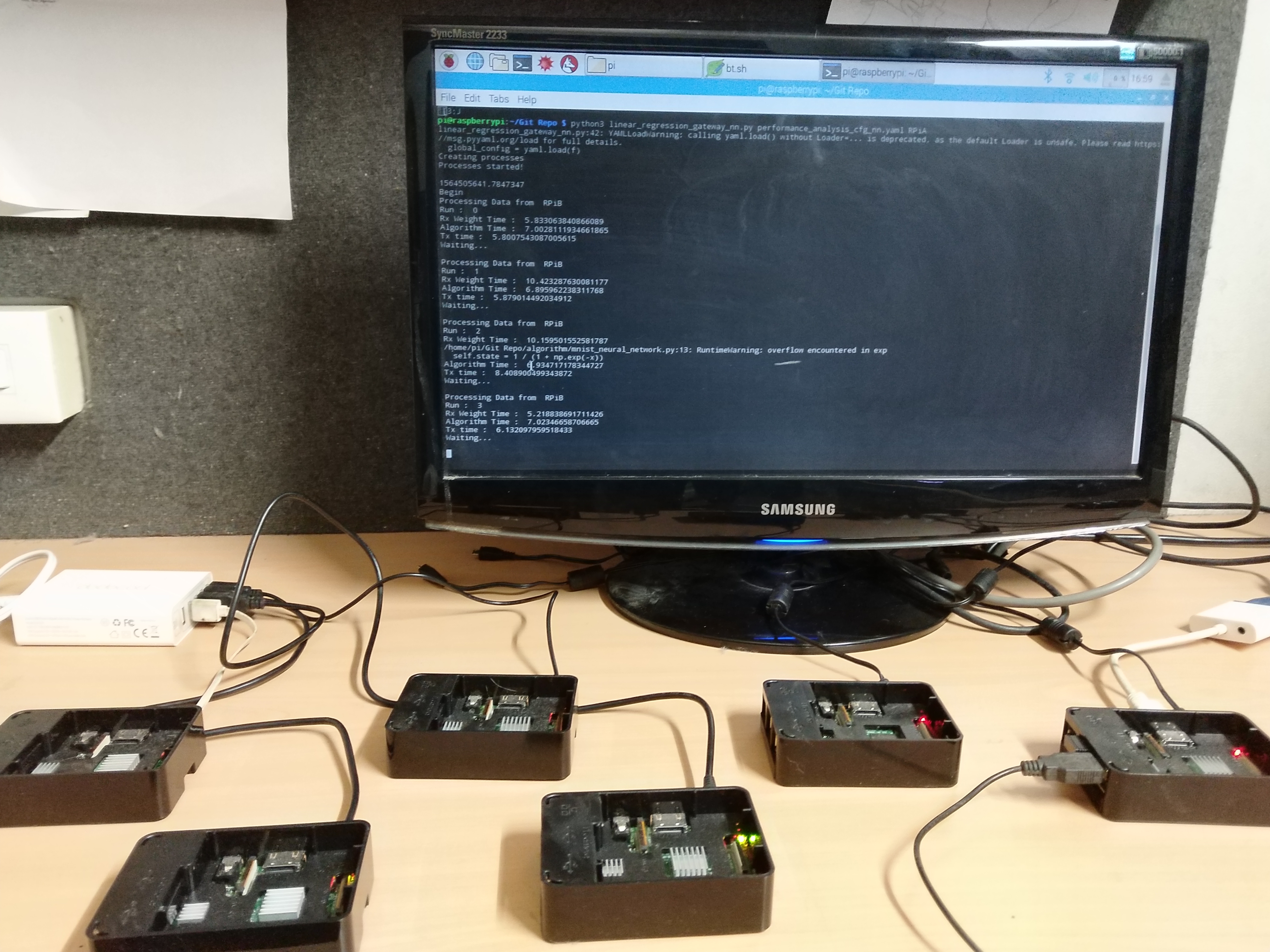
Network cost and capacity parameters. To obtain realistic network costs for nodes and links , we collect measurements from a testbed consisting of six Raspberry Pis as nodes and AWS DynamoDB as a cloud-based parameter server (Figure 3). Three Pis collect data and transmit it over Bluetooth to another “gateway” Pi. The three gateway nodes receive this data and either perform a local gradient update or upload the data to DynamoDB. We measure 100 rounds of gradient update processing times and Pi-to-DynamoDB communication times while training a two-layer fully connected neural network (MLP), with devices communicating over 2.4 GHz WiFi or LTE cellular. These processing times are linearly scaled to range from 0 to 1, and recorded as , while the Pi-to-DynamoDB communication times are similarly scaled and saved as . For completeness, we also evaluate performance for synthetic costs, where we take . Using both types of costs allows for a more thorough comparison between our network-aware and state-of-the-art learning frameworks, as network costs only affect network-aware learning. Unless otherwise stated, results are reported using the testbed-collected parameters.
When imposed, the capacity constraints and are taken as the average data generated per device in each time period, i.e., . The error costs are modeled using the measurements from simulations on the Raspberry Pi testbed. All results are averaged over at least five iterations.
Centralized and federated learning. To see whether our method compromises learning accuracy in considering network costs as additional objectives, we compare against a baseline of centralized ML training where all data is processed at a single device (server). We also compare to federated learning with the same parameters where there is no data offloading or discarding, i.e., .
Perfect information vs. estimation. As discussed in Section IV-A, solving (5-9) in practice requires estimating the costs and capacities over the time horizon . To do this, we divide into intervals , and in each interval , we use the time-averaged observations of , , , and over to compute the optimal data movement. The resulting and for are then used by device to transfer data in . This “imperfect information” scheme will be compared with the ideal case in which the network costs and parameters are available (i.e., “perfect information”).
V-B Efficacy of Network-Aware Learning
We first investigate the efficicacy of our method on a fully-connected network topology .
V-B1 Model accuracy
Table II compares the testing accuracies obtained by centralized, federated, and network-aware learning on both synthetic and testbed network costs. Our method achieves nearly the same (within 4%) accuracy as federated learning in both the i.i.d. and non-i.i.d. cases. The performance differences between the i.i.d. and non-i.i.d. cases of each algorithm are expected, as non-i.i.d. local datasets are not representative of the overall dataset. Note that network-aware learning produced more accurate models on testbed rather than synthetic costs. In practical fog environments, outlined in Section I-A, devices with faster computations are also likely to transmit faster. The testbed-derived real costs contain such a correlation, which allows more cost-effective offloading and improves model accuracy.
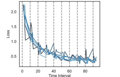
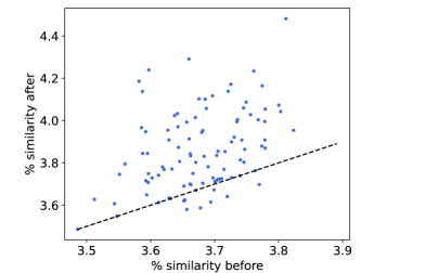
The convergence of network-aware learning across individual devices is shown in Figure 4(a), with all devices exhibiting an overall decreasing trend. In Figure 4(b), we consider the similarity between local data distributions before and after offloading in the non-i.i.d. setting. Percent similarity is calculated between each pair of nodes and as the percent overlap in labels they contain – i.e., where is the multiset of labels at device – and then are averaged over all pairs. The average similarity increases due to offloading in nearly all cases, with an average improvement of around 10%, which is a consequence of data offloading.
| Accuracy (%) | Network costs (both i.i.d. and non-i.i.d.) | ||||||
|---|---|---|---|---|---|---|---|
| i.i.d. | non-i.i.d. | Process | Transfer | Discard | Total | Unit | |
| A | 89.72 | 87.92 | 1234 | 0 | 0 | 1234 | 0.265 |
| B | 89.81 | 81.29 | 322 | 120 | 136 | 578 | 0.118 |
| C | 89.54 | 80.47 | 302 | 117 | 138 | 558 | 0.121 |
| D | 83.14 | 78.25 | 336 | 63 | 187 | 586 | 0.119 |
| E | 82.83 | 77.39 | 307 | 46 | 274 | 627 | 0.136 |
V-B2 Offloading and imperfect information
While network-aware learning obtains similar accuracy to traditional federated learning, we expect it will improve network resource costs. Table III compares the costs incurred and model accuracy for both the i.i.d. and non-i.i.d. scenarios in five settings, where settings B - E are applications of network-aware learning:
-
A.
Offloading and discarding disabled
-
B.
Perfect information and no capacity constraints
-
C.
Imperfect information and no capacity constraints
-
D.
Perfect information and capacity constraints
-
E.
Imperfect information and capacity constraints
Cost components in Table III – process, transfer, and discard (i.e., error) – are summed over all nodes/links and time. The unit cost column is the total cost normalized by the total data generated in that setting, to account for variation in across experiments. Simulations with imperfect information – cases C and E – allocate data based on historical network characteristics, which may be inaccurate, and can cause unintended large transfer or process costs. In the capacity limiting cases – D and E – the excess data must be discarded instead. Note also that the costs are the same for both the i.i.d. and non-i.i.d. settings as our offloading optimization (5)-(9) does not account for local data distributions. Comparing A and B, we see that offloading reduces the unit cost by 53%. The network takes advantage of transfer links, reducing the total processing cost by 74%, by offloading more data. Our model is robust to estimation errors, similar to our observations from Section IV-A, as we observe only minor changes in cost or accuracy from B to C, which has imperfect network information. When devices have strict capacity constraints, as in D and E, their gradient updates are based on fewer samples, and each node’s will tend to have larger errors.
| Discard cost | Accuracy (%) | Network costs | |||||
|---|---|---|---|---|---|---|---|
| objective | i.i.d. | non-i.i.d. | Pr | Tr | Di | Tot | |
| B | 87.89 | 79.68 | 322 | 120 | 136 | 578 | |
| D | 83.14 | 78.25 | 336 | 63 | 187 | 586 | |
| B | 90.05 | 80.90 | 390 | 461 | 125 | 976 | |
| D | 87.86 | 78.08 | 410 | 244 | 136 | 790 | |
| B | 86.81 | 78.04 | 323 | 79 | 172 | 574 | |
| D | 85.42 | 77.26 | 311 | 83 | 184 | 578 | |
Overall, there is a roughly difference in accuracy for the i.i.d. case between settings A and E, and a 13% difference for the non-i.i.d. case; this comes at an improvement of more than 50% in network costs. The accuracy differences for the non-i.i.d. case are larger but exhibit the same trends across settings as the i.i.d. case. If higher accuracy is desired, a different error cost in (5) could be chosen, as we investigate next.
V-B3 Comparing error cost models
We compare the use of three error cost models from Section IV-A: , , and without modification to . For this last case, note that if , as is likely since node is unlikely to offload more data at time than was offloaded to it at . This upper bound on may work well for data-intensive applications as it neglects ’s diminishing marginal returns.
We show the results for the different cost models in Table IV under settings B and D from Table III. The linear cost produces a higher accuracy than using , but incurs a higher total cost due to transfer costs from offloading more data for processing. The results for are close to the convex case. By neglecting the offloading terms in the discard cost, we prevent the solution from offloading more data to further reduce the error cost when it is exceeded by the marginal transfer cost.
V-C Effect of Network System Characteristics
Our next experiments investigate the impact of the number of nodes, , the network connectivity, , and the aggregation period, on network-aware learning. We use a fully connected topology when varying and , and, for varying , we use a random graph with probability .
V-C1 Varying number of nodes
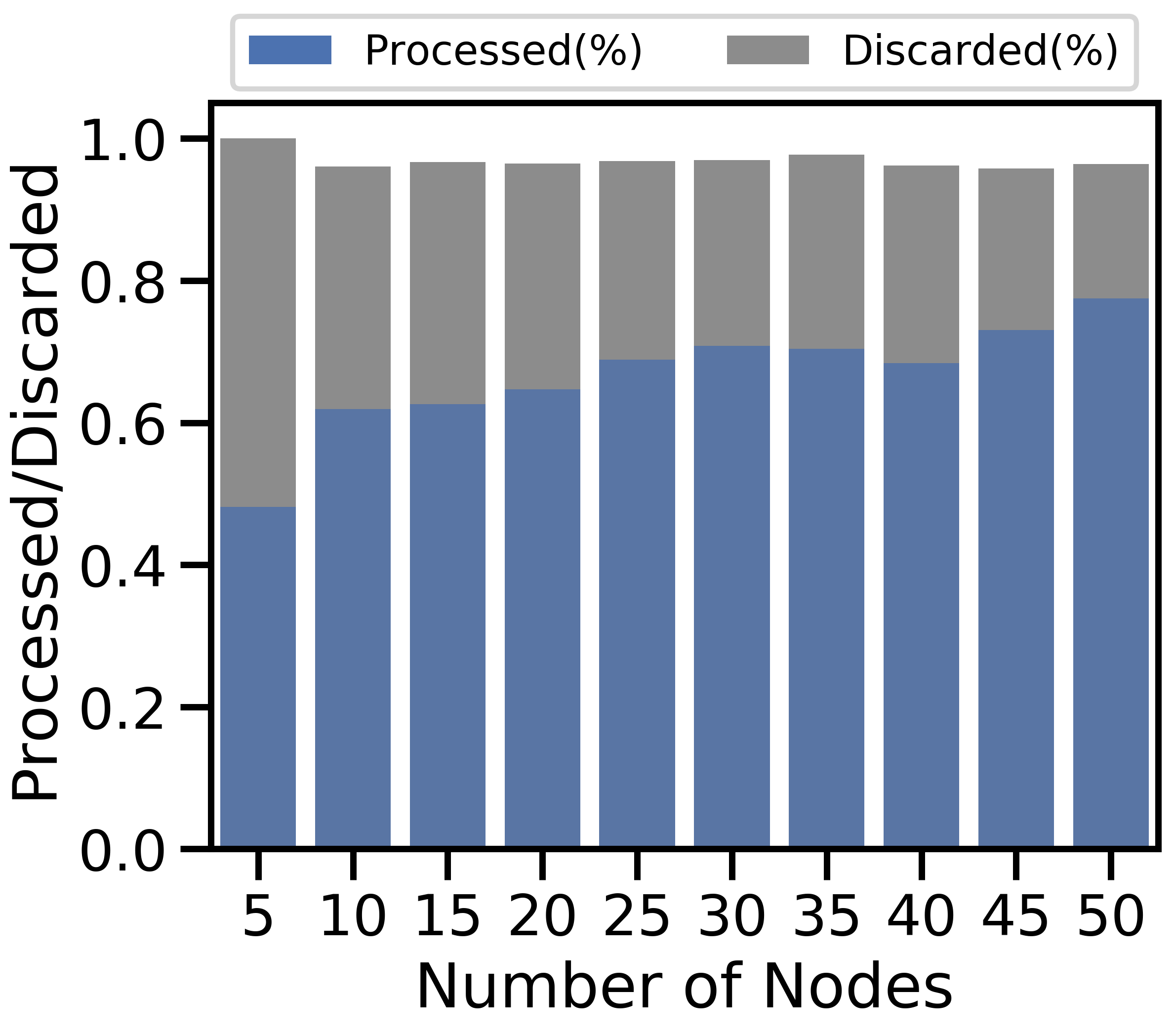
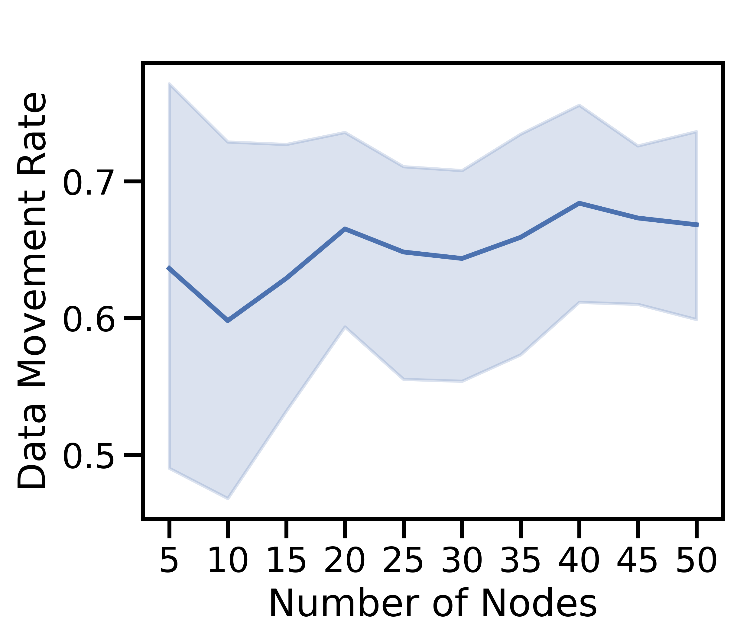
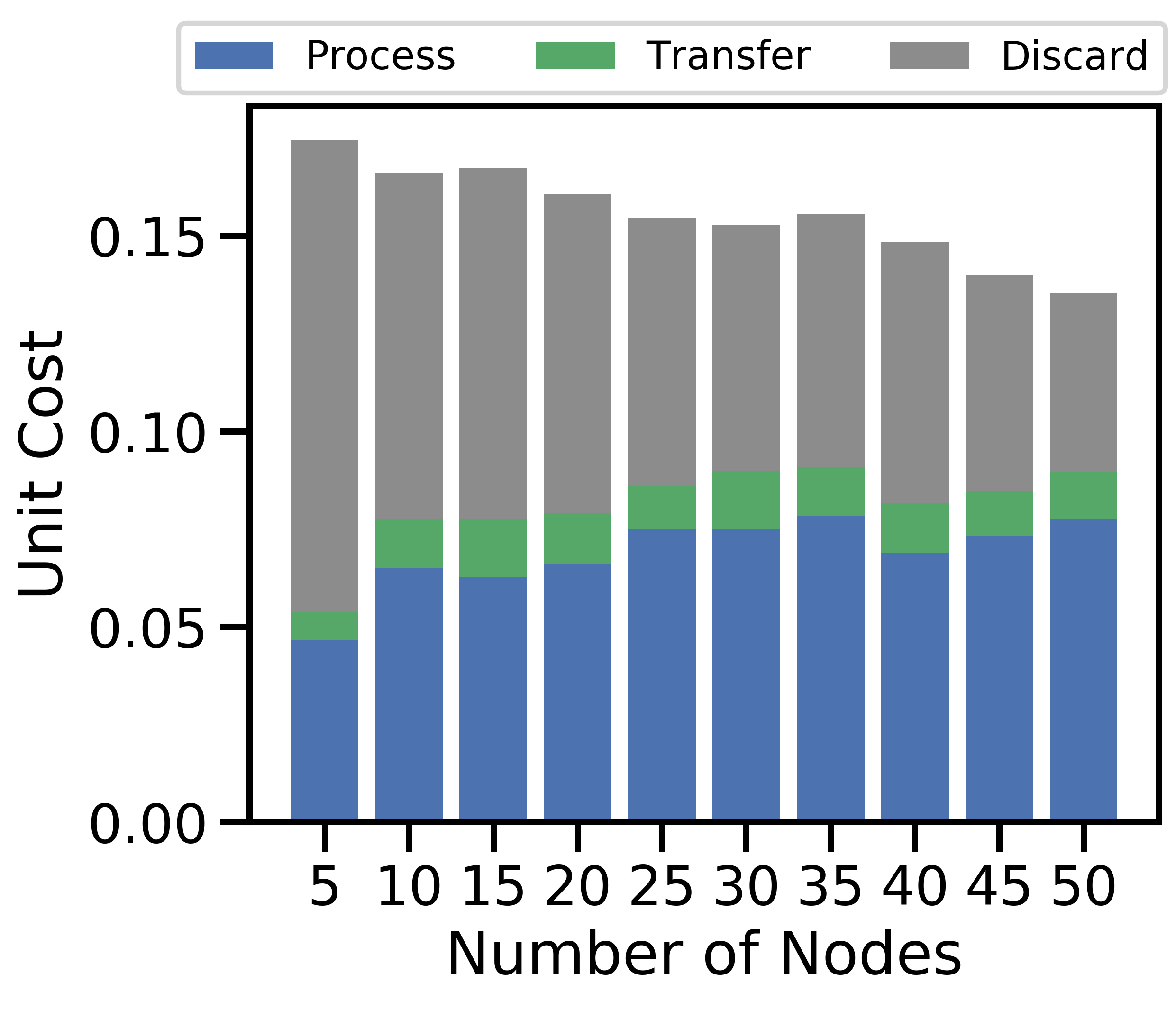
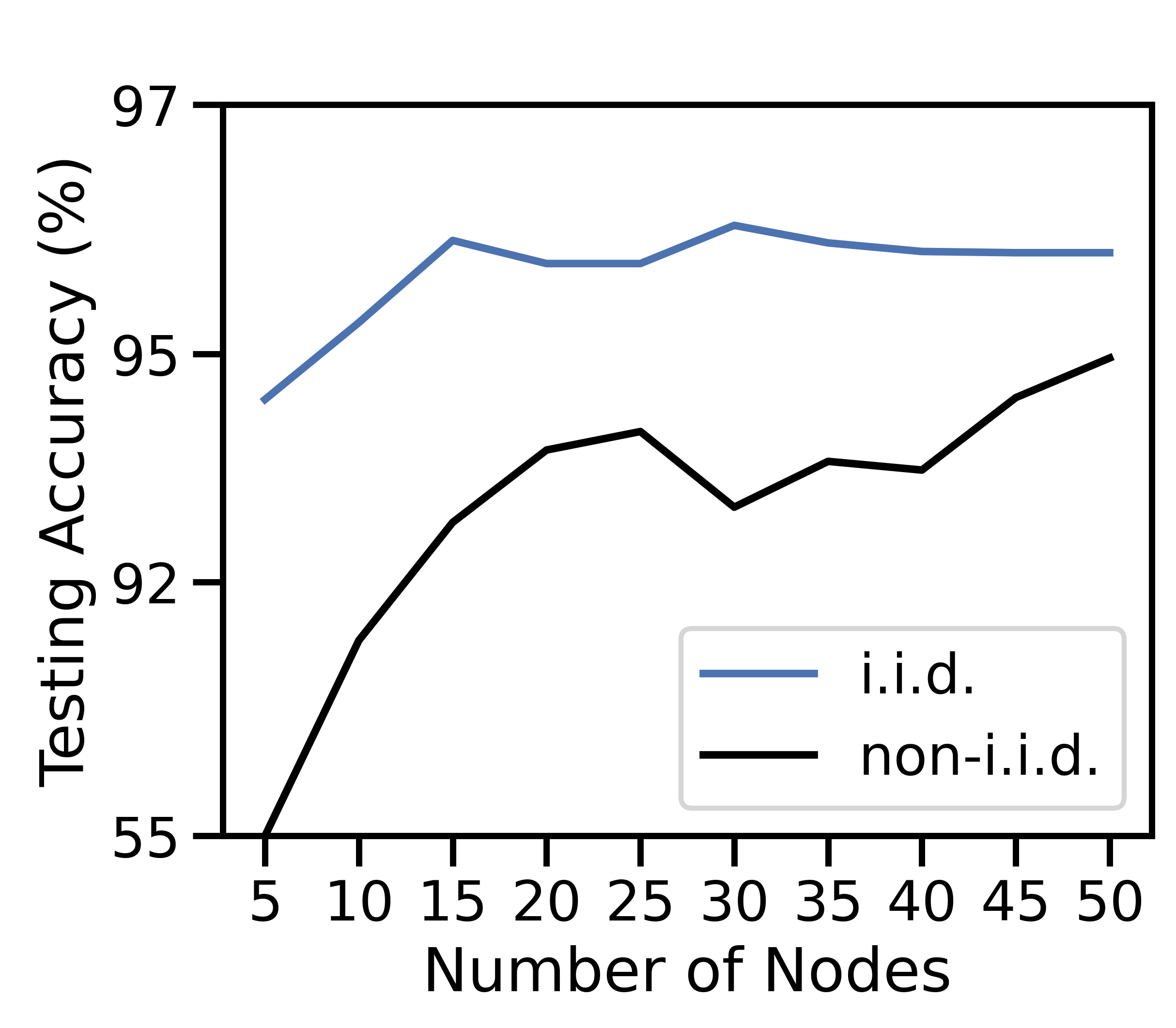
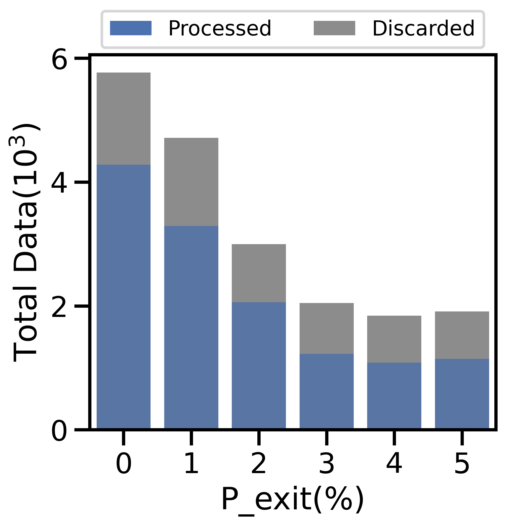
Figure 5 varies from to in increments of five nodes. Figure 5(a) depicts the fraction of data processed vs. discarded333Rounding used during the solution of the optimization problem resulted in the variance in the sum of the processed and discarded data ratios.; 5(b) plots the change in the movement rate, i.e., fraction of data that is either offloaded or discarded; 5(c) breaks down unit cost by component; and 5(d) shows the model accuracy for i.i.d. and non-i.i.d.
Our method scales well as the unit cost in Figure 5(c) decreases with . As the network grows, high-cost nodes are more likely to connect to low-cost nodes, which results in more offloading and is consistent with Theorems 5 and 6. Figure 5(b) confirms this: both the minimum and average data transfer rates grow with network size. As more offloading occurs, more data is processed in Figure 5(a). Although more data is processed, the increased processing cost is outweighed by the savings in discard cost in Figure 5(c). Training on more data then produces a more accurate ML model in Figure 5(d). In Figure 5(d), the non-i.i.d. case shows a substantial accuracy improvement as increases. Since each node in the non-i.i.d. case only contains half of the data labels for the ML problem, small networks are at a natural disadvantage compared to larger ones – their empirical training dataset is unlikely to be representative of the underlying distribution, no matter what offloading scheme is used. Hence, we see the growth from 55% to 95% testing accuracy when increases from 5 to 50.
V-C2 Varying network connectivity
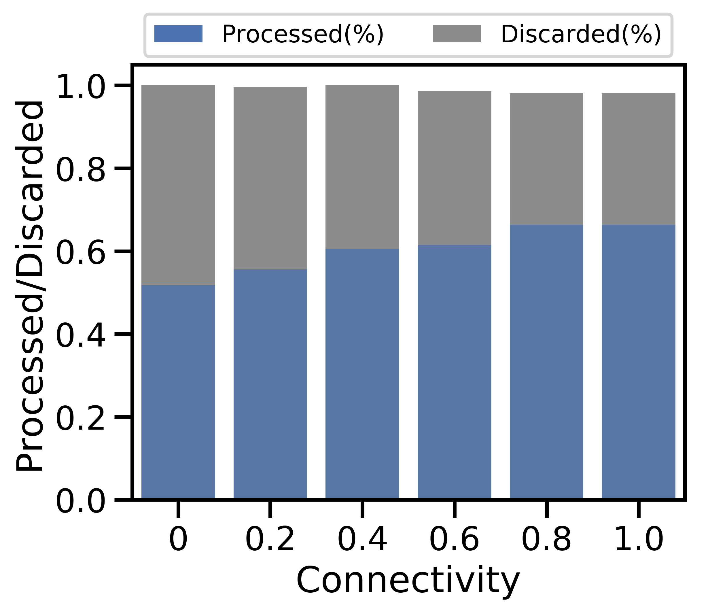
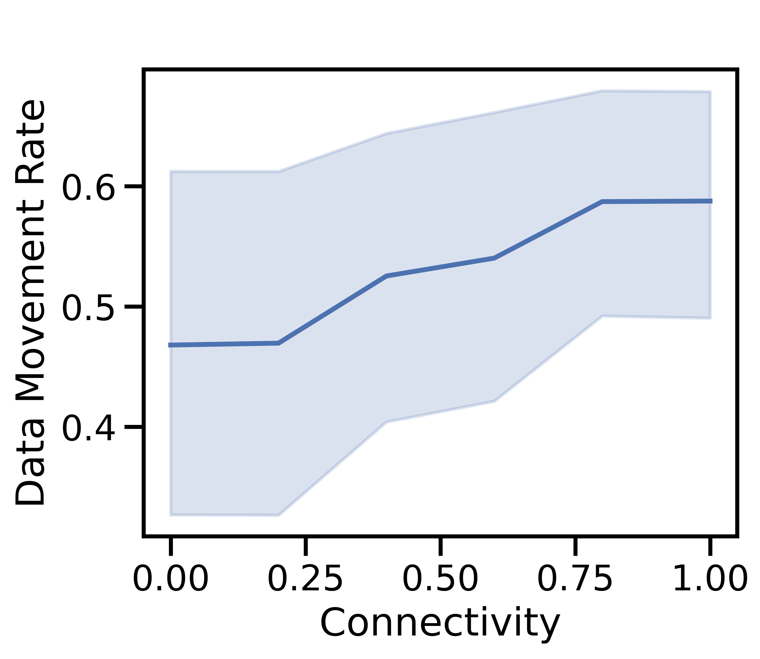
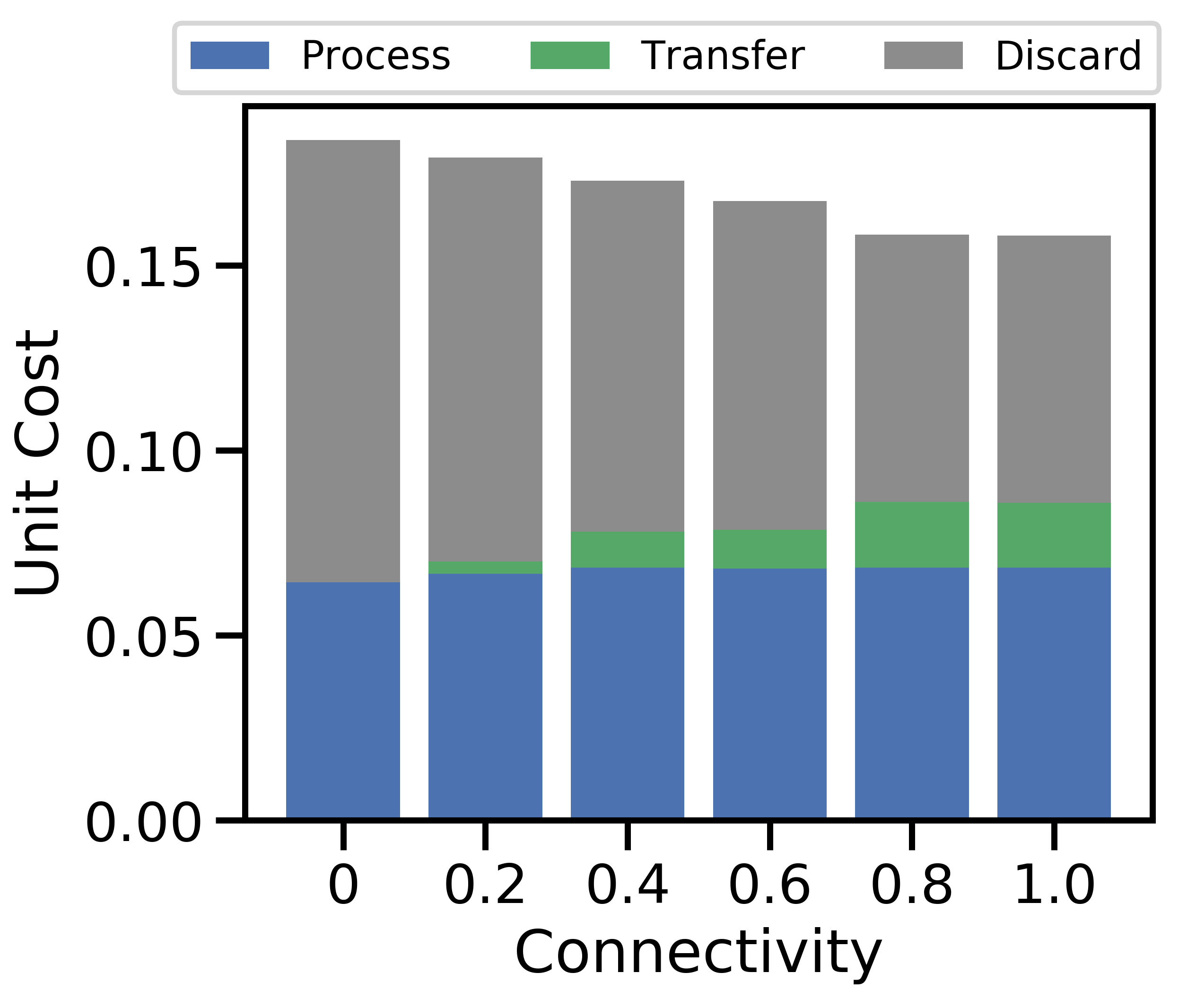
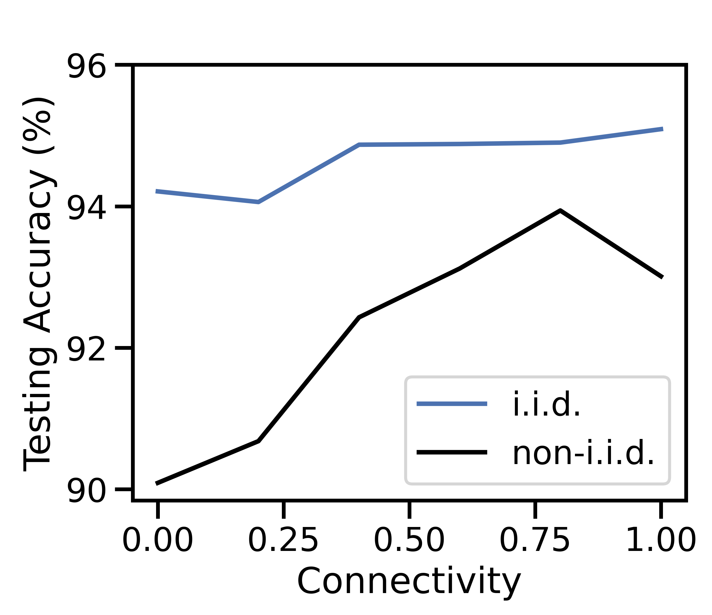
Figure 6 examines the same characteristics in Figure 5 as is varied from (i.e., completely disconnected) to (i.e., fully connected). Overall, we observe a similar trend to the effect of : as connectivity grows, the unit cost per datapoint decreases in Figure 6(c), caused by cheaper alternatives to discarding. The relatively small change in total cost as varies indicates that network-aware learning is robust to variations in device connectivity.
High connectivity produces more opportunities for offloading in Figure 6(b), which increases total data processed and decreases total data discarded in Figure 6(a). Discard costs then take a smaller share of the unit costs in Figure 6(c). Intuitively, more data processed leads to the more accurate model in Figure 6(d). For non-i.i.d. data, the data transfer growth seen in Figures 6(b) and 6(c) increases the dataset similarity among devices, allowing model accuracy to improve. Increased network connectivity has a similar effect to having a larger network: there are more network links to nodes with low processing cost, which network-aware learning can leverage to produce cost savings without compromising model accuracy.
V-C3 Varying aggregation period
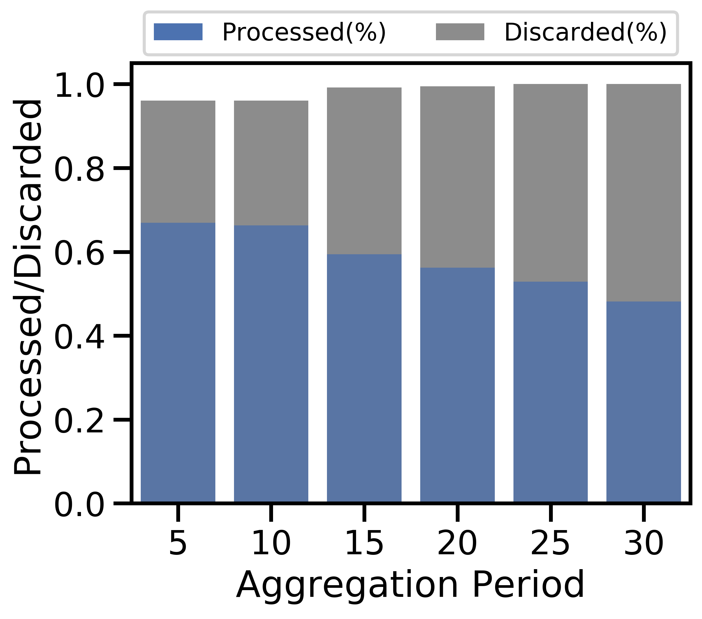
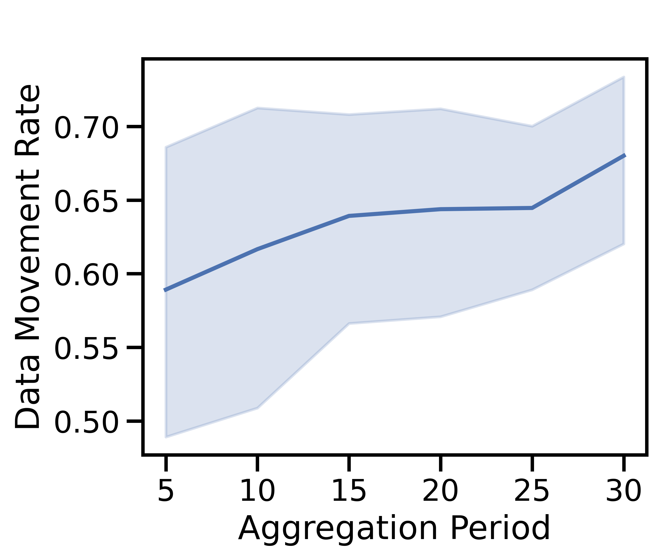
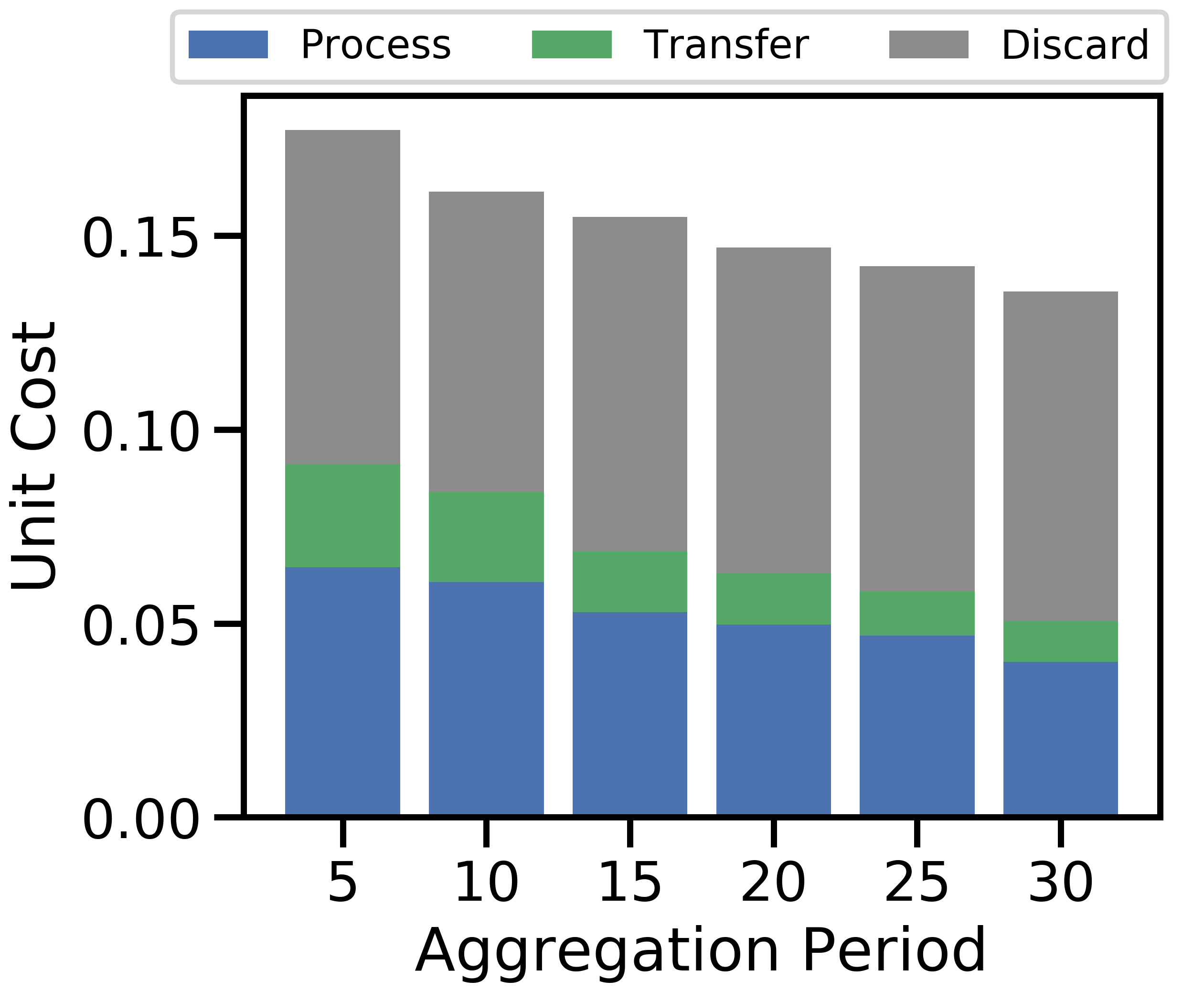
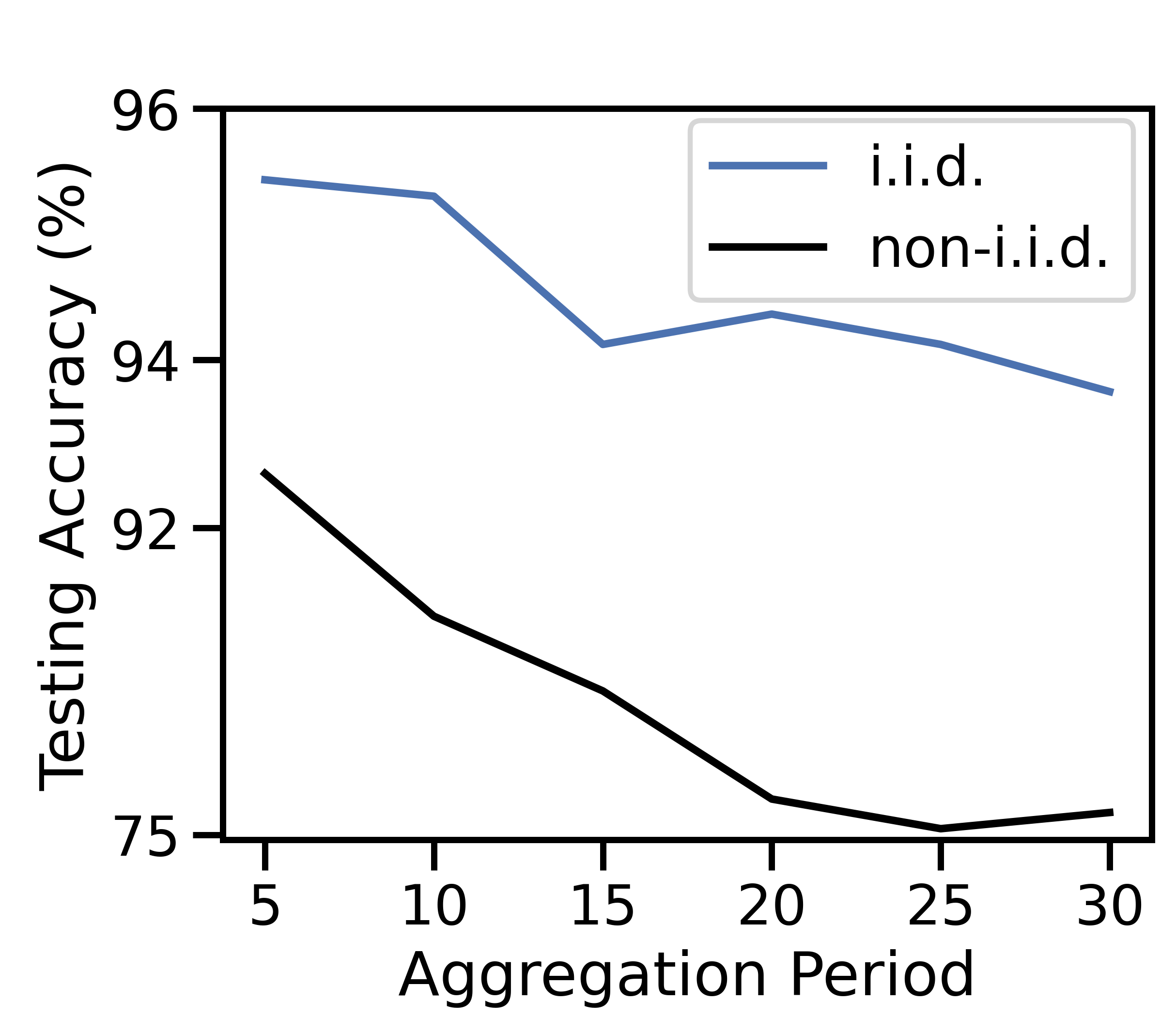
Figure 7 varies the aggregation period . Overall, a larger decreases unit cost and testing accuracy. We expect local models to converge as grows, similar to the effects studied in [5]. As devices train on their local datasets for longer, they begin to converge, reducing the value of processing data. As a result, discarding becomes cost-effective in Figure 7(a), and the discard costs dominate in Figure 7(c), with the data movement rate in Figure 7(b) increasing due to this extra discarding. Finally, since is constant, a higher reduces the number of global aggregations, which results in decreased test accuracy in Figure 7(d), consistent with our findings in Theorem 1. Frequent aggregations are more important in the non-i.i.d. case where aggregations are needed to prevent overfitting to devices’ distinct local distributions. Hence, large results in significantly worse accuracy for non-i.i.d. data.
V-D Effect of Fog Topology
Next, we evaluate network-aware learning on three fog computing topologies: hierarchical and social network topologies as in Section IV-B, and a fully-connected topology in which all nodes are neighbors. The social network is modeled as a Watts-Strogatz small world graph [46] with each node connected to of its neighbors, and the hierarchical network connects each of the nodes with the lowest processing costs to two of the remaining nodes, randomly.
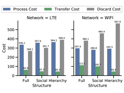
Our Raspberry Pi testbed provides LTE and WiFi network media for which we compare the network resource costs. Both media exhibit similar trends across the topologies in Figure 8. The topology determines offloading availability: the fully-connected topology maximizes the degree of each node, while the hierarchical topology minimizes the average degree. A smaller average degree limits offloading, which leads to more data processed locally and/or discarded. The major difference between LTE and WiFi is that WiFi skews more towards discarding. WiFi has fewer interference mitigation techniques than cellular, so, in the presence of several devices, we expect its links to exhibit longer delays. Consequently, both the discard and transfer costs are larger for WiFi than their LTE counterparts, regardless of topology. Results in both cases are consistent with the findings from varying the network connectivity in Figure 6 too: as networks become less connected and edges grow sparse, the ability of individual devices to offload their data to lower cost alternatives diminishes. Devices will marginally increase their data processing workloads, but ultimately a significant fraction of the data is discarded.
V-E Effect of Dynamic Networks
Finally, we consider network-aware learning when nodes may enter and exit the network. Initially, all devices are in the network. At each , devices in the network will exit with probability , while devices outside the network will re-enter with probability . For worst-case analysis, nodes cannot transmit their local update results prior to exiting, and nodes rejoining the network cannot obtain the current global parameters until the ongoing aggregation period finishes.
| Setting | Acc(%) | Nodes | Cost | |||
|---|---|---|---|---|---|---|
| Process | Transfer | Discard | Unit | |||
| Static | 95.83 | 10 | 399 | 66 | 328 | 0.135 |
| Dynamic | 94.79 | 7.8 | 300 | 56 | 256 | 0.144 |
Table V compares a dynamic network with against the static case. In a dynamic network, network-aware learning operates with less overall network data and compute capability as active nodes per aggregation period decreases from 10 in the static case to an average of 7.8 in the dynamic case. Node exits always result in at least one inactive node - even if a new node enters, it must wait for the synchronized global parameters. So, our methodology is reasonably robust in dynamic networks as a 20% decline in active nodes/period only leads to a 6% increase in unit costs incurred per datapoint, and a 1% accuracy decline, due to fewer processed data and more discarding (also visible from the ratio of processed to discard costs).
V-E1 Varying
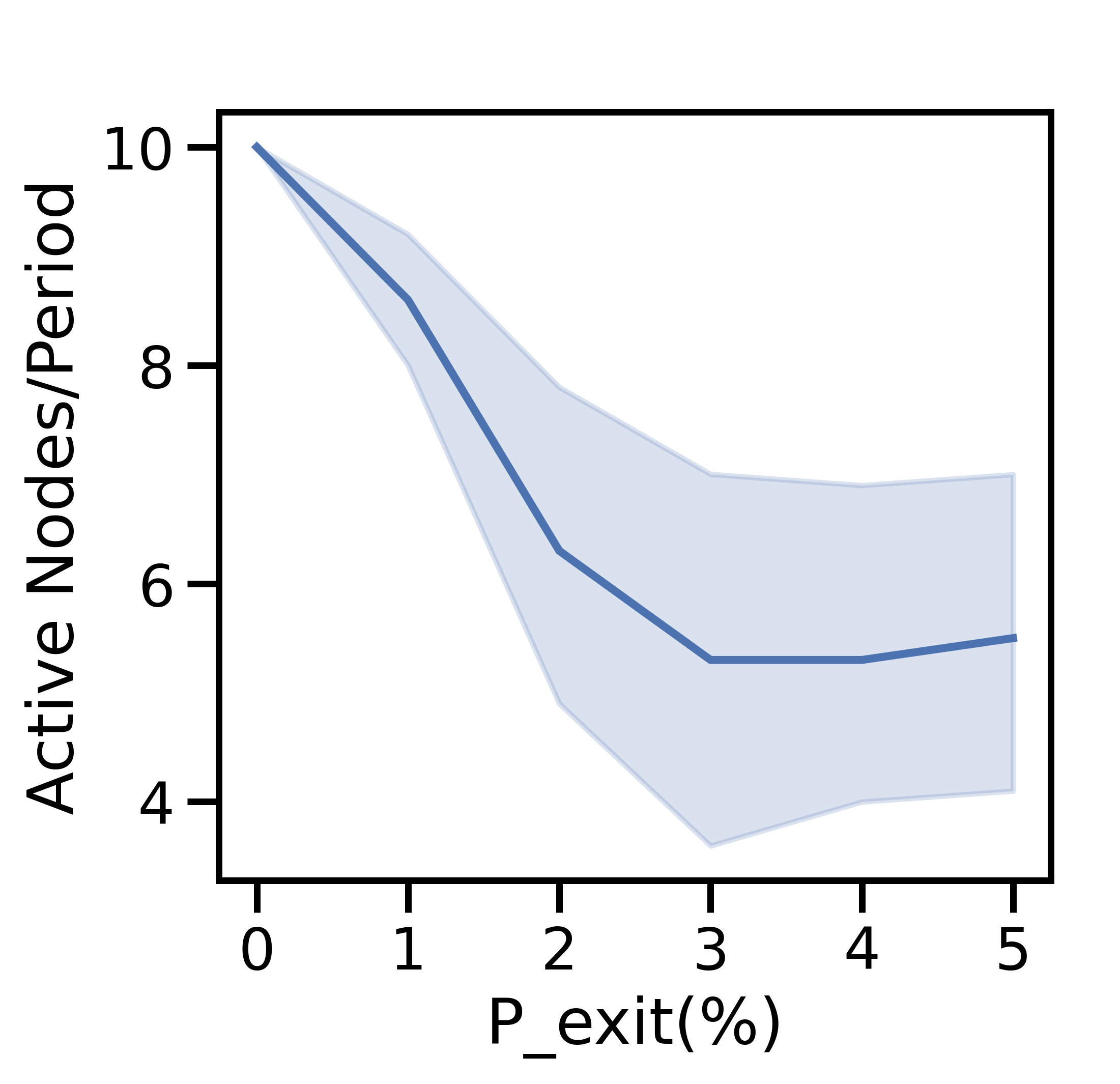
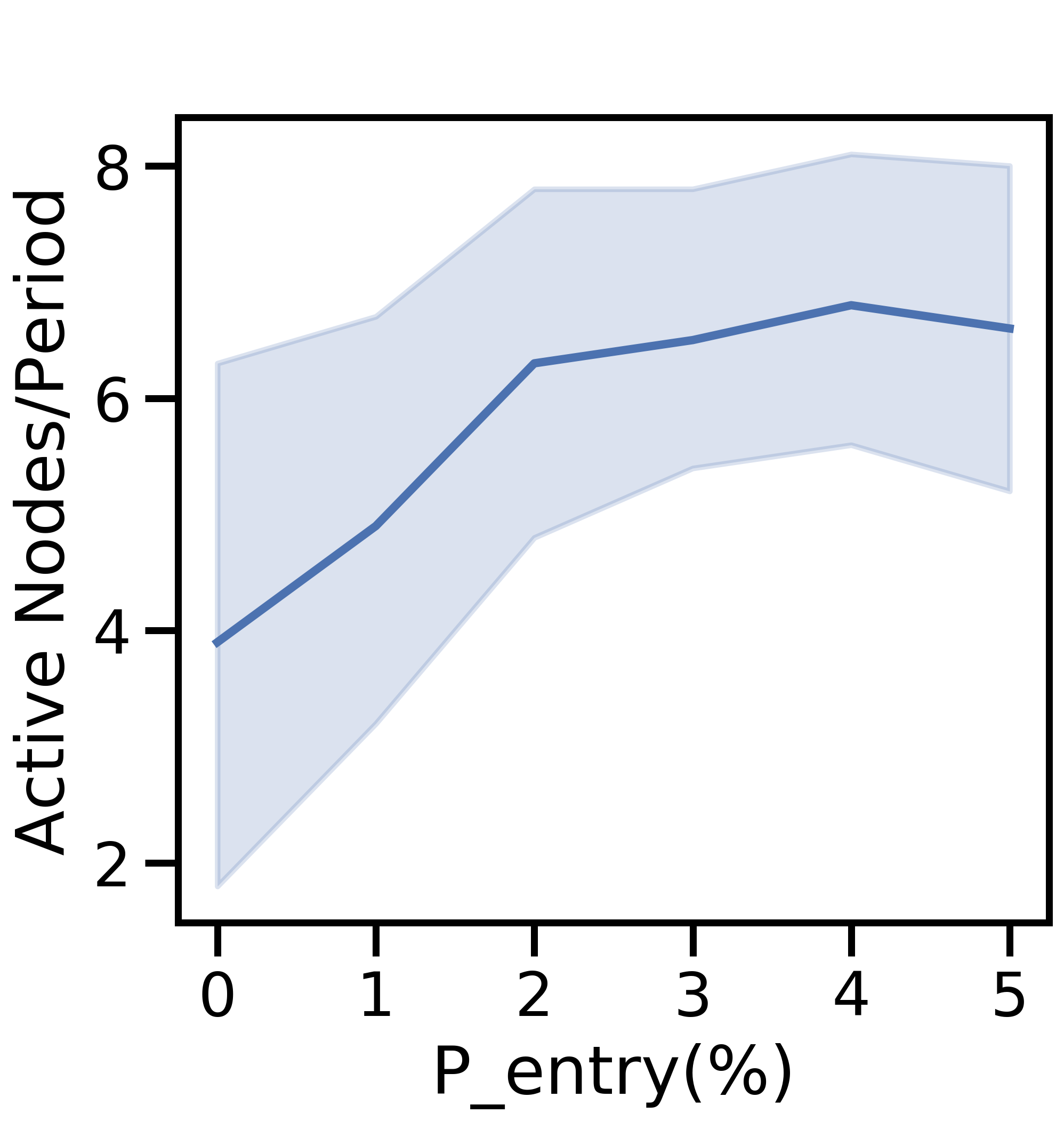
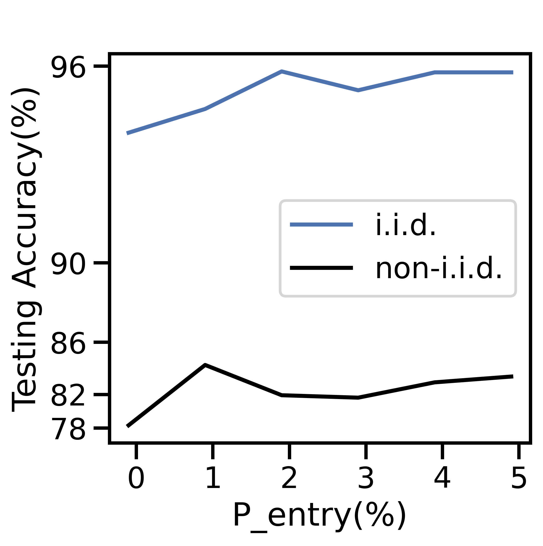
Figure 9 varies from 0-5% and fixes . Figure 9(a) shows the variation in average active nodes per period, and the remaining four subfigures display the aspects of network-aware learning as in Figs. 5-7.
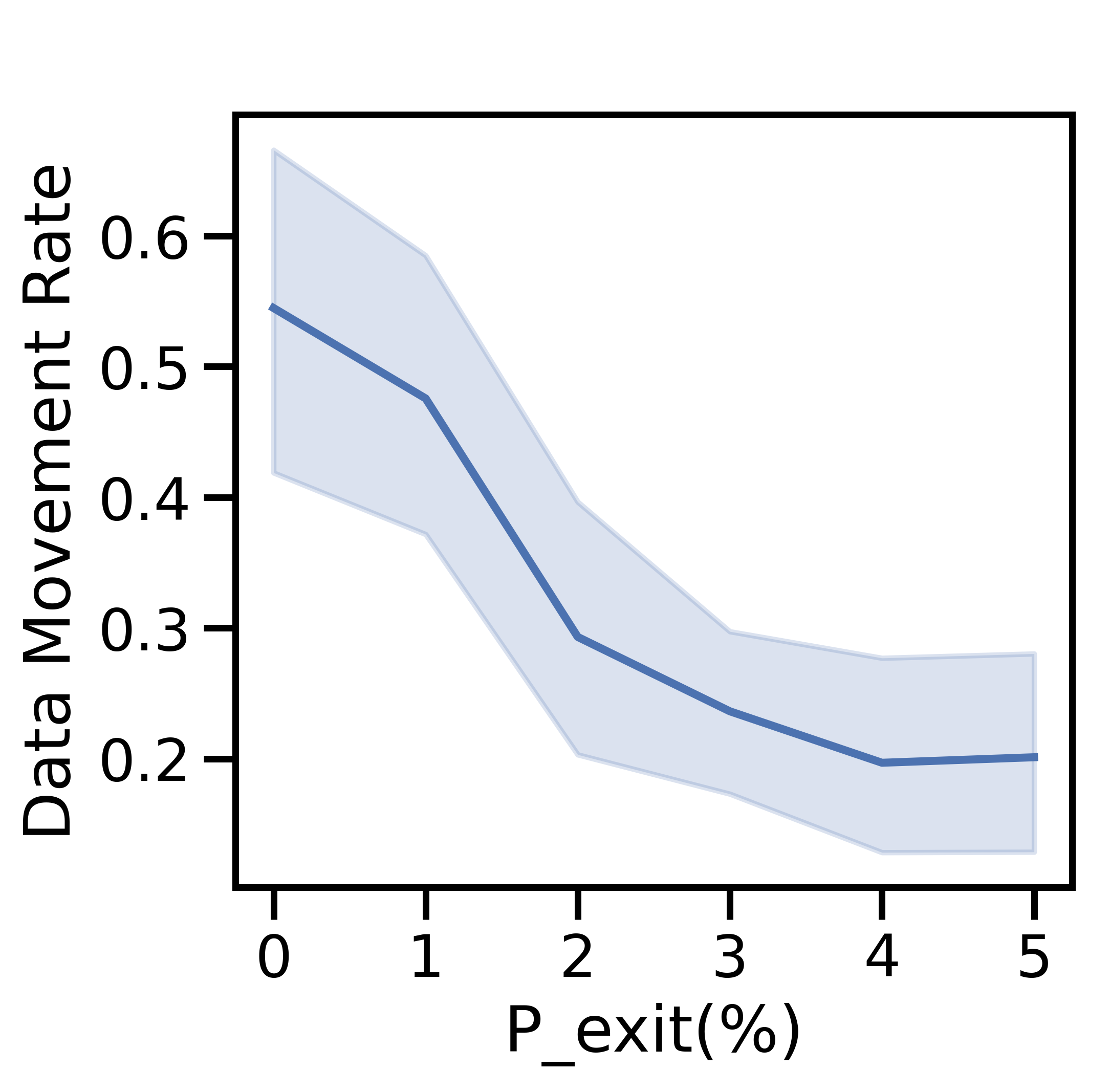
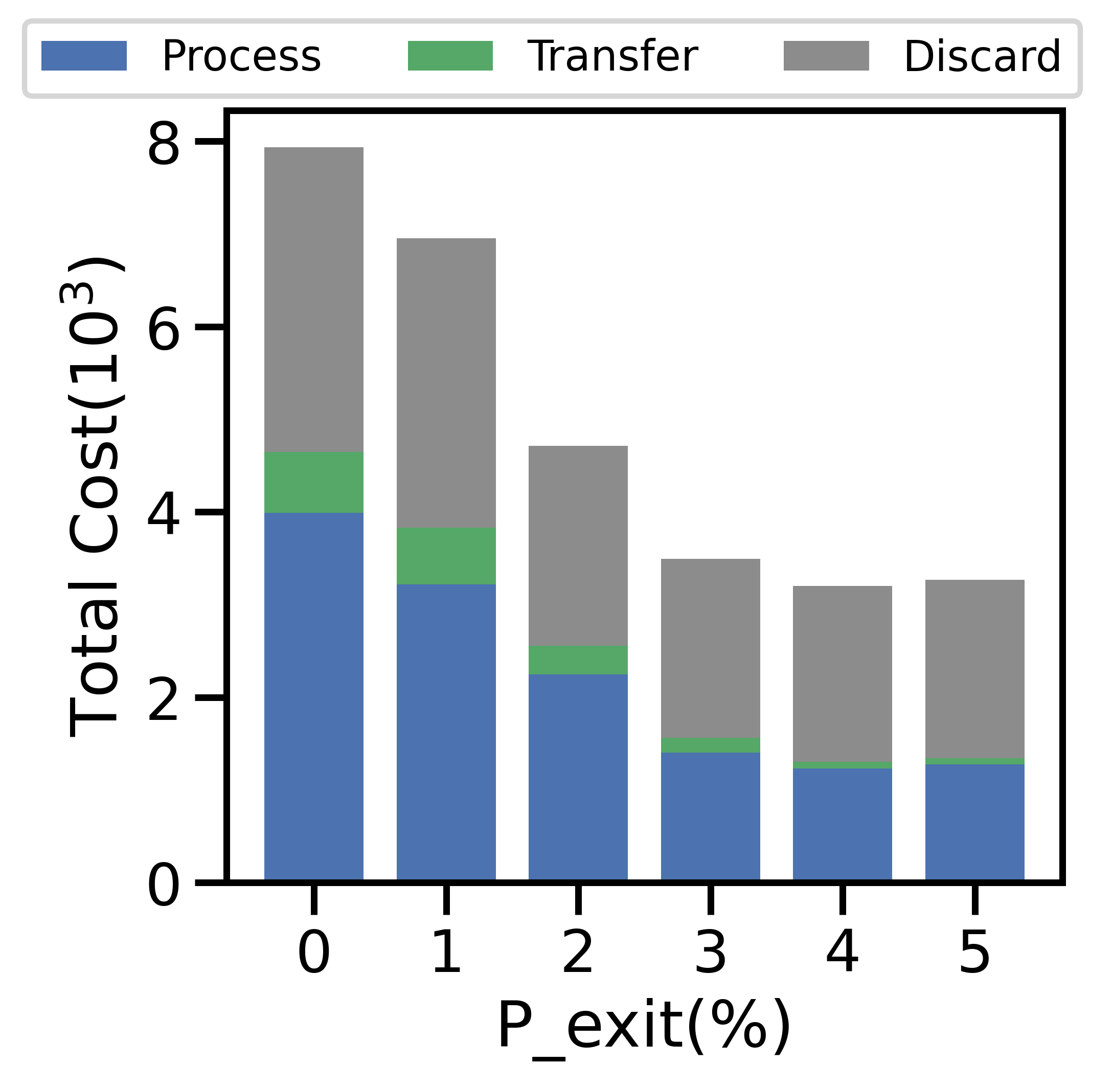
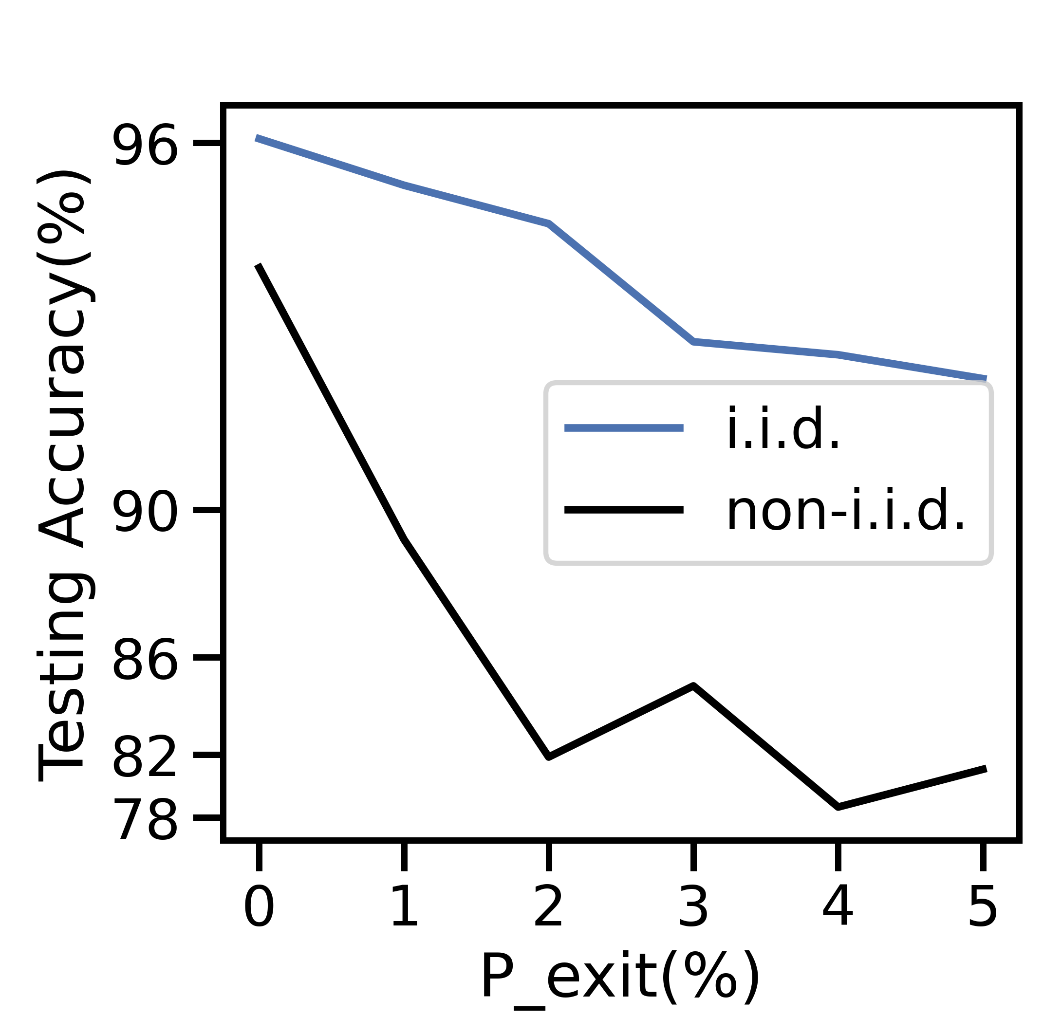
Figure 9(a) depicts a sharp decline in the number of active nodes per period as grows. At , the network averages active nodes/period, a 40% decrease from network initialization. The total generated data and cost decrease sharply in Figures 9(b) and 9(c), respectively: since the network has fewer active nodes, there is less data overall and therefore less cost. While the ratio of processed to discarded data in Figure 9(b) skews towards processed data as increases, the total cost in Figure 9(d) skews toward discard costs: fewer active nodes implies fewer offloading opportunities, and network-aware learning discards more data. As a result, the average data movement rate drops from to in Figure 9(c). The i.i.d. testing accuracy declines by % in Figure 9(e), with a larger decline for non-i.i.d. data.
V-E2 Varying
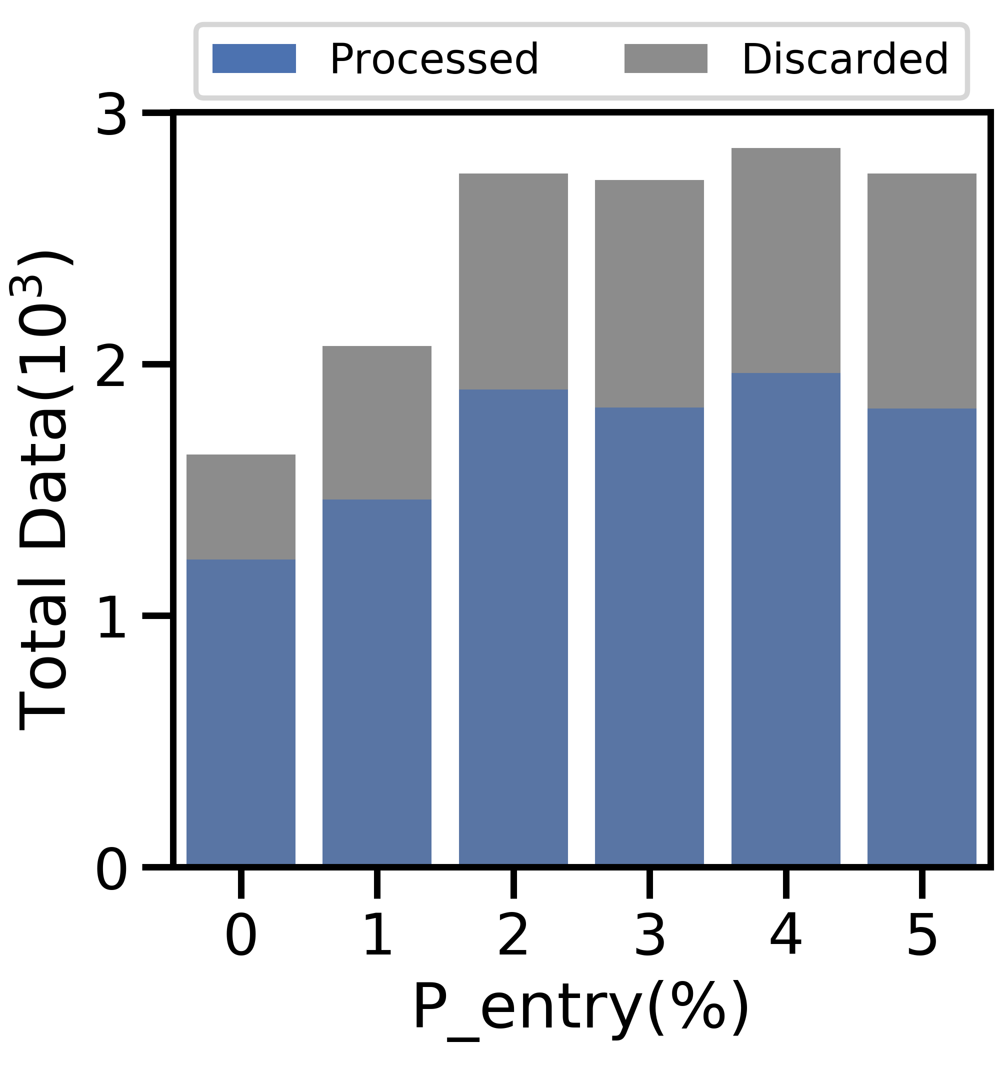
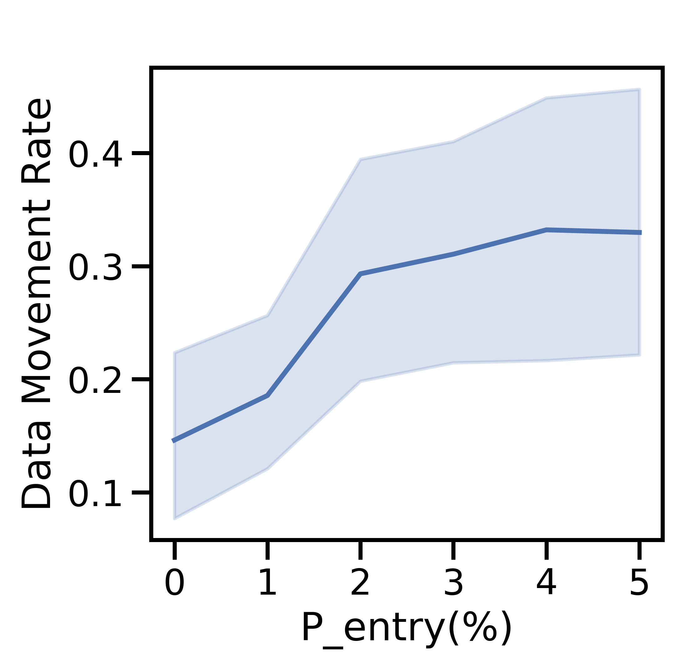
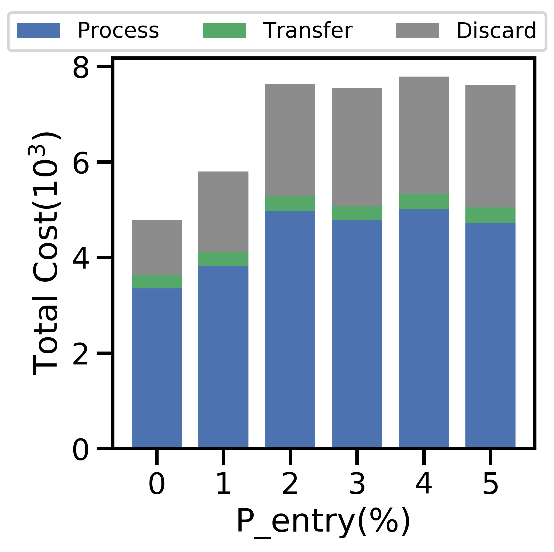
Figure 10 varies from 0-5% with , and the average active nodes per period increases with probability of node entry until 4% in Figure 10(a). Both the total data generated (Figure 10(b)) and average data movement rate (Figure 10(c)) increase with more active nodes, but more data leads to larger processing, discard, and total costs in Figure 10(d). As increases, the network benefits from scale, i.e., more efficient offloading, which enables the network to train a more accurate ML model for the i.i.d. and non-i.i.d. cases in Figure 10(e). However, the overall non-i.i.d. testing accuracy is unable to match that of the i.i.d. case, as node exits distort the distribution of local data across active devices further from the true global distribution.
Figures 9 and 10 exhibit a consistent pattern: the costs rapidly change and then plateau around when for Figure 9 and for Figure 10. For the non-i.i.d. case, we notice that has a stronger effect on the testing accuracy in Figure 9 than does in Figure 10; in the non-i.i.d. case, there is less overlap between devices’ datasets, so each node exit affects the empirical training dataset more substantially and results in a stronger impact on the accuracy.
VI Conclusion and Future Work
In this paper, we developed a novel methodology to distribute ML training tasks over devices in a fog computing network while considering the compute-communication-accuracy tradeoffs inherent in fog scenarios. We derived new error bounds when devices transfer their local data processing to each other, and bounded the impact of these transfers on the cost and accuracy of the model training. Through experimentation with a popular machine learning task, we showed that our network-aware scheme significantly reduces the cost of model training while achieving comparable accuracy to the recently popularized federated learning algorithm for distributed training, and demonstrated the effects of network characteristics and device data distributions on its performance.
Our framework and analysis point to several possible extensions. First, while we do not observe significant heterogeneity in compute times on our wireless testbed, in general fog devices may experience compute straggling and failures, which might benefit from more sophisticated offloading mechanisms. Second, predicting devices’ mobility patterns and network connectivity could likely further optimize the data offloading. Finally, learning device-specific models when local distributions are non-i.i.d. could introduce new performance tradeoffs between offloading and data processing.
Acknowledgment
This work was partially supported by NSF CNS-1909306, by ARO grant W911NF1910036, and by NSWC Crane. We thank the anonymous reviewers for their valuable comments.
References
- [1] Y. Tu, Y. Ruan, S. Wagle, C. Brinton, and C. Joe-Wong, “Network-Aware Optimization of Distributed Learning for Fog Computing,” in IEEE INFOCOM, 2020.
- [2] Cisco Systems, “Demystifying 5G in Industrial IOT,” White Paper, 2019. [Online]. Available: https://www.cisco.com/c/dam/en_us/solutions/iot/demystifying-5g-industrial-iot.pdf
- [3] D. Chatzopoulos, C. Bermejo, Z. Huang, and P. Hui, “Mobile Augmented Reality Survey: From where we are to where we go,” IEEE Access, vol. 5, pp. 6917–6950, 2017.
- [4] K. Rao, “The Path to 5G for Health Care,” IEEE Perspectives on 5G Applications and Services. [Online]. Available: https://futurenetworks.ieee.org/images/files/pdf/applications/5G--Health-Care030518.pdf
- [5] S. Wang, T. Tuor, T. Salonidis, K. K. Leung, C. Makaya, T. He, and K. Chan, “Adaptive Federated Learning in Resource Constrained Edge Computing Systems,” IEEE JSAC, vol. 37, no. 6, pp. 1205–1221, 2019.
- [6] M. Chiang and T. Zhang, “Fog and IoT: An Overview of Research Opportunities,” IEEE Int. Things J., vol. 3, no. 6, pp. 854–864, 2016.
- [7] IEEE Spectrum, “Applications of Device-to-Device Communication in 5G Networks,” White Paper. [Online]. Available: https://spectrum.ieee.org/computing/networks/applications-of-devicetodevice-communication-in-5g-networks
- [8] M. Somisetty, “Big Data Analytics in 5G,” IEEE Perspectives on 5G Applications and Services. [Online]. Available: https://futurenetworks.ieee.org/images/files/pdf/applications/Data-Analytics-in-5G-Applications030518.pdf
- [9] S. Pu, W. Shi, J. Xu, and A. Nedić, “A Push-Pull Gradient Method for Distributed Optimization in Networks,” in IEEE Conference on Decision and Control (CDC), 2018, pp. 3385–3390.
- [10] H. B. McMahan, E. Moore, D. Ramage, S. Hampson, and B. A. y Arcas, “Communication-Efficient Learning of Deep Networks from Decentralized Data,” in AISTATS, 2017.
- [11] T.-Y. Yang, C. Brinton, P. Mittal, M. Chiang, and A. Lan, “Learning Informative and Private Representations via Generative Adversarial Networks,” in IEEE Intl. Conf. on Big Data. IEEE, 2018, pp. 1534–1543.
- [12] S. A. Ashraf, I. Aktas, E. Eriksson, K. W. Helmersson, and J. Ansari, “Ultra-Reliable and Low-Latency Communication for Wireless Factory Automation: From LTE to 5G,” in IEEE International Conference on Emerging Technologies and Factory Automation (ETFA), 2016, pp. 1–8.
- [13] L. He, A. Bian, and M. Jaggi, “Cola: Decentralized linear learning,” in NeurIPS, 2018, pp. 4536–4546.
- [14] J. B. Predd, S. R. Kulkarni, and H. V. Poor, “A collaborative training algorithm for distributed learning,” IEEE Transactions on Information Theory, vol. 55, no. 4, pp. 1856–1871, 2009.
- [15] H. Tang, C. Yu, C. Renggli, S. Kassing, A. Singla, D. Alistarh, J. Liu, and C. Zhang, “Distributed learning over unreliable networks,” ArXiv, vol. abs/1810.07766, 2019.
- [16] S. Dutta, G. Joshi, S. Ghosh, P. Dube, and P. Nagpurkar, “Slow and Stale Gradients Can Win the Race: Error-Runtime Trade-offs in Distributed SGD,” in AISTATS, 2018, pp. 803–812.
- [17] J. Konečnỳ, H. B. McMahan, F. X. Yu, P. Richtárik, A. T. Suresh, and D. Bacon, “Federated Learning: Strategies for Improving Communication Efficiency,” in NeurIPS, 2016.
- [18] R. Shokri and V. Shmatikov, “Privacy-Preserving Deep Learning,” in ACM SIGSAC, 2015, pp. 1310–1321.
- [19] S. A. Rahman, H. Tout, H. Ould-Slimane, A. Mourad, C. Talhi, and M. Guizani, “A survey on federated learning: The journey from centralized to distributed on-site learning and beyond,” IEEE Internet of Things Journal, 2020.
- [20] V. Smith, C.-K. Chiang, M. Sanjabi, and A. S. Talwalkar, “Federated Multi-Task Learning,” in NeurIPS, 2017, pp. 4424–4434.
- [21] Y. Zhao, M. Li, L. Lai, N. Suda, D. Civin, and V. Chandra, “Federated Learning with Non-IID Data,” arXiv:1806.00582, 2018.
- [22] G. Neglia, G. Calbi, D. Towsley, and G. Vardoyan, “The Role of Network Topology for Distributed Machine Learning,” in IEEE Conference on Computer Communications (INFOCOM), 2019, pp. 2350–2358.
- [23] J. Konečný, H. B. McMahan, F. X. Yu, P. Richtárik, A. T. Suresh, and D. Bacon, “Federated learning: Strategies for improving communication efficiency,” 2016.
- [24] N. Strom, “Scalable distributed dnn training using commodity gpu cloud computing,” in Sixteenth Annual Conference of the International Speech Communication Association, 2015.
- [25] A. F. Aji and K. Heafield, “Sparse communication for distributed gradient descent,” Proceedings of the 2017 Conference on EMNLP, 2017. [Online]. Available: http://dx.doi.org/10.18653/v1/D17-1045
- [26] F. Sattler, S. Wiedemann, K.-R. Müller, and W. Samek, “Robust and communication-efficient federated learning from non-iid data,” 2019.
- [27] Y. Chen, X. Sun, and Y. Jin, “Communication-efficient federated deep learning with asynchronous model update and temporally weighted aggregation,” 2019.
- [28] A. Lalitha, O. C. Kilinc, T. Javidi, and F. Koushanfar, “Peer-to-peer federated learning on graphs,” 2019.
- [29] N. H. Tran, W. Bao, A. Zomaya, M. N. H. Nguyen, and C. S. Hong, “Federated Learning over Wireless Networks: Optimization Model Design and Analysis,” in IEEE INFOCOM, 2019, pp. 1387–1395.
- [30] T. Chang, L. Zheng, M. Gorlatova, C. Gitau, C.-Y. Huang, and M. Chiang, “Demo: Decomposing Data Analytics in Fog Networks,” in ACM Conference on Embedded Networked Sensor Systems (SenSys), 2017.
- [31] X. Ran, H. Chen, X. Zhu, Z. Liu, and J. Chen, “DeepDecision: A Mobile Deep Learning Framework for Edge Video Analytics,” in IEEE INFOCOM, 2018, pp. 1421–1429.
- [32] C. Hu, W. Bao, D. Wang, and F. Liu, “Dynamic Adaptive DNN Surgery for Inference Acceleration on the Edge,” in IEEE INFOCOM, 2019, pp. 1423–1431.
- [33] S. Teerapittayanon, B. McDanel, and H.-T. Kung, “Distributed Deep Neural Networks over the Cloud, the Edge and End Devices,” in IEEE ICDCS, 2017, pp. 328–339.
- [34] X. Xu, D. Li, Z. Dai, S. Li, and X. Chen, “A heuristic offloading method for deep learning edge services in 5g networks,” IEEE Access, vol. 7, pp. 67 734–67 744, 2019.
- [35] H. Li, K. Ota, and M. Dong, “Learning iot in edge: Deep learning for the internet of things with edge computing,” IEEE Network, vol. 32, pp. 96–101, 2018.
- [36] Y. Sun, S. Zhou, and D. Gündüz, “Energy-aware analog aggregation for federated learning with redundant data,” in IEEE ICC. IEEE, 2020, pp. 1–7.
- [37] T. Yang, “Trading Computation for Communication: Distributed Stochastic Dual Coordinate Ascent,” in NeurIPS, 2013, pp. 629–637.
- [38] Y. Zhang, J. Duchi, M. I. Jordan, and M. J. Wainwright, “Information-theoretic Lower Bounds for Distributed Statistical Estimation with Communication Constraints,” in NeurIPS, 2013, pp. 2328–2336.
- [39] K. P. Murphy, Machine Learning: A Probabilistic Perspective. MIT Press, 2012.
- [40] F. Farhat, D. Z. Tootaghaj, Y. He, A. Sivasubramaniam, M. Kandemir, and C. R. Das, “Stochastic Modeling and Optimization of Stragglers,” IEEE Trans. on Cloud Comp,, vol. 6, no. 4, pp. 1164–1177, 2016.
- [41] F. M. F. Wong, Z. Liu, and M. Chiang, “On the Efficiency of Social Recommender Networks,” IEEE/ACM Trans. Netw., vol. 24, pp. 2512–2524, 2016.
- [42] C. A. Bouman and K. Sauer, “A unified approach to statistical tomography using coordinate descent optimization,” IEEE Transactions on image processing, vol. 5, no. 3, pp. 480–492, 1996.
- [43] A. Nadh, J. Samuel, A. Sharma, S. Aniruddhan, and R. K. Ganti, “A taylor series approximation of self-interference channel in full-duplex radios,” IEEE Trans. Wirls. Comm., vol. 16, no. 7, pp. 4304–4316, 2017.
- [44] Y. LeCun, C. Cortes, and C. J. C. Burges, “The MNIST Database of Handwritten Digits.” [Online]. Available: http://yann.lecun.com/exdb/mnist/
- [45] Y. LeCun, B. Boser, J. S. Denker, D. Henderson, R. E. Howard, W. Hubbard, and L. D. Jackel, “Backpropagation Applied to Handwritten Zip Code Recognition,” Neural Comp., vol. 1, no. 4, pp. 541–551, 1989.
- [46] M. Chiang, Networked Life: 20 Questions and Answers. Cambridge University Press, 2012.
| Su Wang is a second year PhD student in Electrical and Computer Engineering at Purdue University. He received his BS in Electrical Engineering from Purdue in 2018. |
| Yichen Ruan is a Ph.D. candidate in Electrical and Computer Engineering at Carnegie Mellon University. He received his B.S. and M.S. degrees respectively from Tsinghua University and UC Berkeley. |
| Yuwei Tu is an independent researcher conducting research on machine learning and network optimization. She graduated from the Center of Data Science at New York University with a master degree of data science. |
| Satyavrat Wagle is a researcher in the Software Systems and Services Research Area (SSS-RA) at Tata Consultancy Services (TCS) Research. He holds an MS in Electrical Engineering from Carnegie Mellon University. |
| Christopher G. Brinton (SM’20) is an Assistant Professor of Electrical and Computer Engineering at Purdue University. He received his PhD degree in Electrical Engineering from Princeton University in 2016. Since joining Purdue in 2019, he has won several awards including the Seed for Success Award and the Ruth and Joel Spira Outstanding Teacher Award. |
| Carlee Joe-Wong (M’16) is the Robert E. Doherty Assistant Professor of Electrical and Computer Engineering at Carnegie Mellon University. She received her A.B., M.A., and Ph.D. degrees from Princeton University in 2011, 2013, and 2016, respectively. She has received several awards for her work, including the Army Young Investigator and NSF CAREER awards. |
Appendix A Proofs of All Theorems
A-A Proof of Theorem 1
Proof:
To aid in analysis, we define for as the centralized version of the gradient descent update synchronized with the weighted average after every global aggregation , i.e., . With , letting , we can write
| (17) |
where the three inequalities use the results , , and from Lemma 2 in [5]. Here, and for . Additionally, if we assume , we can write
| (18) |
where the inequality uses the result for any from Lemma 3 in [5], and the -Lipschitz assumption on which extends to by the triangle inequality, i.e., for any . Adding the results from (17) and (18) and noting , we have
Taking the reciprocal, it follows that
| (19) |
for . Now, let be the positive root of , which is easy to check exists. We can show that one of the following conditions must be true: (i) or (ii) . If we assume is non-increasing with , then from (i) and (ii) we can write or . But we already know for any , so with the -Lipschitz assumption . If (ii) holds, then, . Now comparing (i) and (ii), (ii) must always be true since . ∎
A-B Proof of Theorem 2
Proof:
Since we assume all costs and capacities are constant, we first note that the can also be assumed to be constant. Thus, the processing of data at node can be modeled as a D/M/1 queue, with constant arrival rate and exponential service time. The expected waiting time of such a queue is then equal to , where is the smallest solution to . Upon showing that the expected waiting time is an increasing function of and an increasing function of , it follows that to ensure an expected waiting time no larger than , we should choose , where is the maximum arrival rate such that . ∎
A-C Proof of Theorem 4
Proof:
In the hierarchical scenario described in the statement of the theorem, the cost objective (5) can be rewritten as
Taking the partial derivative of the cost objective with respect to and setting to 0 gives:
Rearranging gives , which yields:
Using the expression for , the objective function becomes:
Taking the partial derivative with respect to and setting to gives:
Since at the optimal point, and we obtain for each . We can then enforce for all and rearrange for to obtain:
Finally, note that a large forces , which gives the result. ∎
A-D Proof of Theorem 5
Proof:
From Theorem 3, we can write the expected cost savings as
|
|
(20) |
where we take and use the fact that the minimum of i.i.d. uniform random variables on has the probability distribution . Integrating and simplifying then yields the desired result.
∎