Tobias Heuer, Peter Sanders and Sebastian Schlag
Network Flow-Based Refinement for Multilevel Hypergraph Partitioning
Abstract.
We present a refinement framework for multilevel hypergraph partitioning that uses max-flow computations on pairs of blocks to improve the solution quality of a -way partition. The framework generalizes the flow-based improvement algorithm of KaFFPa from graphs to hypergraphs and is integrated into the hypergraph partitioner KaHyPar. By reducing the size of hypergraph flow networks, improving the flow model used in KaFFPa, and developing techniques to improve the running time of our algorithm, we obtain a partitioner that computes the best solutions for a wide range of benchmark hypergraphs from different application areas while still having a running time comparable to that of hMetis.
Key words and phrases:
multilevel hypergraph partitioning, network flows, refinement1991 Mathematics Subject Classification:
G.2.2 Graph Theory, G.2.3 Applications1. Introduction
Given an undirected hypergraph , the -way hypergraph partitioning problem is to partition the vertex set into disjoint blocks of bounded size (at most times the average block size) such that an objective function involving the cut hyperedges is minimized. Hypergraph partitioning (HGP) has many important applications in practice such as scientific computing [12] or VLSI design [43]. Particularly VLSI design is a field where small improvements can lead to significant savings [56].
It is well known that HGP is NP-hard [38], which is why practical applications mostly use heuristic multilevel algorithms [11, 13, 25, 26]. These algorithms successively contract the hypergraph to obtain a hierarchy of smaller, structurally similar hypergraphs. After applying an initial partitioning algorithm to the smallest hypergraph, contraction is undone and, at each level, a local search method is used to improve the partitioning induced by the coarser level. All state-of-the-art HGP algorithms [2, 4, 7, 16, 28, 31, 32, 33, 48, 51, 52, 54] either use variations of the Kernighan-Lin (KL) [34, 49] or the Fiduccia-Mattheyses (FM) heuristic [19, 46], or simpler greedy algorithms [32, 33] for local search. These heuristics move vertices between blocks in descending order of improvements in the optimization objective (gain) and are known to be prone to get stuck in local optima when used directly on the input hypergraph [33]. The multilevel paradigm helps to some extent, since it allows a more global view on the problem on the coarse levels and a very fine-grained view on the fine levels of the multilevel hierarchy. However, the performance of move-based approaches degrades for hypergraphs with large hyperedges. In these cases, it is difficult to find meaningful vertex moves that improve the solution quality because large hyperedges are likely to have many vertices in multiple blocks [53]. Thus the gain of moving a single vertex to another block is likely to be zero [41].
While finding balanced minimum cuts in hypergraphs is NP-hard, a minimum cut separating two vertices can be found in polynomial time using network flow algorithms and the well-known max-flow min-cut theorem [21]. Flow algorithms find an optimal min-cut and do not suffer the drawbacks of move-based approaches. However, they were long overlooked as heuristics for balanced partitioning due to their high complexity [40, 57]. In the context of graph partitioning, Sanders and Schulz [47] recently presented a max-flow-based improvement algorithm which is integrated into the multilevel partitioner KaFFPa and computes high quality solutions.
Outline and Contribution.
Motivated by the results of Sanders and Schulz [47], we generalize the max-flow min-cut refinement framework of KaFFPa from graphs to hypergraphs. After introducing basic notation and giving a brief overview of related work and the techniques used in KaFFPa in Section 2, we explain how hypergraphs are transformed into flow networks and present a technique to reduce the size of the resulting hypergraph flow network in Section 3.1. In Section 3.2 we then show how this network can be used to construct a flow problem such that the min-cut induced by a max-flow computation between a pair of blocks improves the solution quality of a -way partition. We furthermore identify shortcomings of the KaFFPa approach that restrict the search space of feasible solutions significantly and introduce an advanced model that overcomes these limitations by exploiting the structure of hypergraph flow networks. We implemented our algorithm in the open source HGP framework KaHyPar and therefore briefly discuss implementation details and techniques to improve the running time in Section 3.3. Extensive experiments presented in Section 4 demonstrate that our flow model yields better solutions than the KaFFPa approach for both hypergraphs and graphs. We furthermore show that using pairwise flow-based refinement significantly improves partitioning quality. The resulting hypergraph partitioner, KaHyPar-MF, performs better than all competing algorithms on all instance classes and still has a running time comparable to that of hMetis. On a large benchmark set consisting of 3222 instances from various application domains, KaHyPar-MF computes the best partitions in 2427 cases.
2. Preliminaries
2.1. Notation and Definitions
An undirected hypergraph is defined as a set of vertices and a set of hyperedges/nets with vertex weights and net weights , where each net is a subset of the vertex set (i.e., ). The vertices of a net are called pins. We extend and to sets, i.e., and . A vertex is incident to a net if . denotes the set of all incident nets of . The degree of a vertex is . The size of a net is the number of its pins. Given a subset , the subhypergraph is defined as .
A -way partition of a hypergraph is a partition of its vertex set into blocks such that , for , and for . We call a -way partition -balanced if each block satisfies the balance constraint: for some parameter . For each net , denotes the connectivity set of . The connectivity of a net is . A net is called cut net if . Given a -way partition of , the quotient graph contains an edge between each pair of adjacent blocks. The -way hypergraph partitioning problem is to find an -balanced -way partition of a hypergraph that minimizes an objective function over the cut nets for some . Several objective functions exist in the literature [5, 38]. The most commonly used cost functions are the cut-net metric and the connectivity metric [1], where is the set of all cut nets [17]. In this paper, we use the -metric. Optimizing both objective functions is known to be NP-hard [38]. Hypergraphs can be represented as bipartite graphs [29]. In the following, we use nodes and edges when referring to graphs and vertices and nets when referring to hypergraphs. In the bipartite graph the vertices and nets of form the node set and for each net , we add an edge to . The edge set is thus defined as . Each net in therefore corresponds to a star in .
Let be a weighted directed graph. We use the same notation as for hypergraphs to refer to node weights , edge weights , and node degrees . Furthermore denotes the neighbors of node . A path is a sequence of nodes, such that each pair of consecutive nodes is connected by an edge. A strongly connected component is a set of nodes such that for each there exists a path from to . A topological ordering is a linear ordering of such that every directed edge implies in the ordering. A set of nodes is called a closed set iff there are no outgoing edges leaving , i.e., if the conditions and imply . A subset is called a node separator if its removal divides into two disconnected components.
A flow network is a directed graph with two distinguished nodes and in which each edge has a capacity . An -flow (or flow) is a function that satisfies the capacity constraint , the skew symmetry constraint , and the flow conservation constraint . The value of a flow is defined as the total amount of flow transferred from to . The residual capacity is defined as . Given a flow , with is the residual network. An -cut (or cut) is a bipartition of a flow network with and . The capacity of an -cut is defined as , where . The max-flow min-cut theorem states that the value of a maximum flow is equal to the capacity of a minimum cut separating and [21].
2.2. Related Work
Hypergraph Partitioning.
Driven by applications in VLSI design and scientific computing, HGP has evolved into a broad research area since the 1990s. We refer to [5, 8, 43, 50] for an extensive overview. Well-known multilevel HGP software packages with certain distinguishing characteristics include PaToH [12] (originating from scientific computing), hMetis [32, 33] (originating from VLSI design), KaHyPar [2, 28, 48] (general purpose, -level), Mondriaan [54] (sparse matrix partitioning), MLPart [4] (circuit partitioning), Zoltan [16], Parkway [51] and SHP [31] (distributed), UMPa [52] (directed hypergraph model, multi-objective), and kPaToH (multiple constraints, fixed vertices) [7]. All of these tools either use variations of the Kernighan-Lin (KL) [34, 49] or the Fiduccia-Mattheyses (FM) heuristic [19, 46], or algorithms that greedily move vertices [33] or nets [32] to improve solution quality in the refinement phase.
Flows on Hypergraphs.
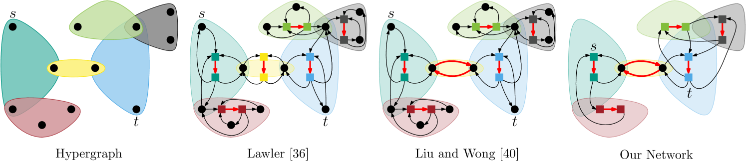
While flow-based approaches have not yet been considered as refinement algorithms for multilevel HGP, several works deal with flow-based hypergraph min-cut computation. The problem of finding minimum -cuts in hypergraphs was first considered by Lawler [36], who showed that it can be reduced to computing maximum flows in directed graphs. Hu and Moerder [29] present an augmenting path algorithm to compute a minimum-weight vertex separator on the star-expansion of the hypergraph. Their vertex-capacitated network can also be transformed into an edge-capacitated network using a transformation due to Lawler [37]. Yang and Wong [57] use repeated, incremental max-flow min-cut computations on the Lawler network [36] to find -balanced hypergraph bipartitions. Solution quality and running time of this algorithm are improved by Lillis and Cheng [39] by introducing advanced heuristics to select source and sink nodes. Furthermore, they present a preflow-based [22] min-cut algorithm that implicitly operates on the star-expanded hypergraph. Pistorius and Minoux [45] generalize the algorithm of Edmonds and Karp [18] to hypergraphs by labeling both vertices and nets. Liu and Wong [40] simplify Lawler’s hypergraph flow network [36] by explicitly distinguishing between graph edges and hyperedges with three or more pins. This approach significantly reduces the size of flow networks derived from VLSI hypergraphs, since most of the nets in a circuit are graph edges. Note that the above-mentioned approaches to model hypergraphs as flow networks for max-flow min-cut computations do not contradict the negative results of Ihler et al. [30], who show that, in general, there does not exist an edge-weighted graph that correctly represents the min-cut properties of the corresponding hypergraph .
Flow-Based Graph Partitioning.
Flow-based refinement algorithms for graph partitioning include Improve [6] and MQI [35], which improve expansion or conductance of bipartitions. MQI also yields as small improvement when used as a post processing technique on hypergraph bipartitions initially computed by hMetis [35]. FlowCutter [24] uses an approach similar to Yang and Wong [57] to compute graph bisections that are Pareto-optimal in regard to cut size and balance. Sanders and Schulz [47] present a flow-based refinement framework for their direct -way graph partitioner KaFFPa. The algorithm works on pairs of adjacent blocks and constructs flow problems such that each min-cut in the flow network is a feasible solution in regard to the original partitioning problem.
KaHyPar.
Since our algorithm is integrated into the KaHyPar framework, we briefly review its core components. While traditional multilevel HGP algorithms contract matchings or clusterings and therefore work with a coarsening hierarchy of levels, KaHyPar instantiates the multilevel paradigm in the extreme -level version, removing only a single vertex between two levels. After coarsening, a portfolio of simple algorithms is used to create an initial partition of the coarsest hypergraph. During uncoarsening, strong localized local search heuristics based on the FM algorithm [19, 46] are used to refine the solution. Our work builds on KaHyPar-CA [28], which is a direct -way partitioning algorithm for optimizing the -metric. It uses an improved coarsening scheme that incorporates global information about the community structure of the hypergraph into the coarsening process.
2.3. The Flow-Based Improvement Framework of KaFFPa
We discuss the framework of Sanders and Schulz [47] in greater detail, since our work makes use of the techniques proposed by the authors. For simplicity, we assume . The techniques can be applied on a -way partition by repeatedly executing the algorithm on pairs of adjacent blocks. To schedule these refinements, the authors propose an active block scheduling algorithm, which schedules blocks as long as their participation in a pairwise refinement step results in some changes in the -way partition.
An -balanced bipartition of a graph is improved with flow computations as follows. The basic idea is to construct a flow network based on the induced subgraph , where is a set of nodes around the cut of . The size of is controlled by an imbalance factor , where is a scaling parameter that is chosen adaptively depending on the result of the min-cut computation. If the heuristic found an -balanced partition using , the cut is accepted and is increased to where is a predefined upper bound. Otherwise it is decreased to . This scheme continues until a maximal number of rounds is reached or a feasible partition that did not improve the cut is found.
In each round, the corridor is constructed by performing two breadth-first searches (BFS). The first BFS is done in the induced subgraph . It is initialized with the boundary nodes of and stops if would exceed . The second BFS constructs in an analogous fashion using . Let be the border of . Then is constructed by connecting all border nodes of to the source and all border nodes to the sink using directed edges with an edge weight of . By connecting and to the respective border nodes, it is ensured that edges incident to border nodes, but not contained in , cannot become cut edges. For , the size of thus ensures that the flow network has the cut property, i.e., each -min-cut in yields an -balanced partition of with a possibly smaller cut. For larger values of , this does not have to be the case.
After computing a max-flow in , the algorithm tries to find a min-cut with better balance. This is done by exploiting the fact that one -max-flow contains information about all -min-cuts [44]. More precisely, the algorithm uses the 1–1 correspondence between -min-cuts and closed sets containing in the Picard-Queyranne-DAG of the residual graph [44]. First, is constructed by contracting each strongly connected component of the residual graph. Then the following heuristic (called most balanced minimum cuts) is repeated several times using different random seeds. Closed node sets containing are computed by sweeping through the nodes of in reverse topological order (e.g. computed using a randomized DFS). Each closed set induces a differently balanced min-cut and the one with the best balance (with respect to the original balance constraint) is used as resulting bipartition.
3. Hypergraph Max-Flow Min-Cut Refinement
In the following, we generalize the flow-based refinement algorithm of KaFFPa to hypergraph partitioning. In Section 3.1 we first show how hypergraph flow networks are constructed in general and introduce a technique to reduce their size by removing low-degree hypernodes. Given a -way partition of a hypergraph , a pair of blocks adjacent in the quotient graph , and a corridor , Section 3.2 then explains how is used to build a flow problem based on a -induced subhypergraph . The flow problem is constructed such that an -max-flow computation optimizes the cut metric of the bipartition of and thus improves the -metric in . Section 3.3 then discusses the integration into KaHyPar and introduces several techniques to speed up flow-based refinement. Algorithm 1 gives a pseudocode description of the entire flow-based refinement framework.
3.1. Hypergraph Flow Networks
The Liu-Wong Network [40].
Given a hypergraph and two distinct nodes and , an -min-cut can be computed by finding a minimum-capacity cut in the following flow network :
-
•
contains all vertices in .
-
•
For each multi-pin net with , add two bridging nodes and to and a bridging edge with capacity to . For each pin , add two edges and with capacity to .
-
•
For each two-pin net , add two bridging edges and with capacity to .
The flow network of Lawler [36] does not distinguish between two-pin and multi-pin nets. This increases the size of the network by two vertices and three edges per two-pin net. Figure 1 shows an example of the Lawler and Liu-Wong hypergraph flow networks as well as of our network described in the following paragraph.
Removing Low Degree Hypernodes.
We further decrease the size of the network by using the observation that the problem of finding an -min-cut of can be reduced to finding a minimum-weight -vertex-separator in the star-expansion, where the capacity of each star-node is the weight of the corresponding net and all other nodes (corresponding to vertices in ) have infinite capacity [29]. Since the separator has to be a subset of the star-nodes, it is possible to replace any infinite-capacity node by adding a clique between all adjacent star-nodes without affecting the separator. The key observation now is that an infinite-capacity node with degree induces infinite-capacity edges in the Lawler network [36], while a clique between star-nodes induces edges. For hypernodes with , it therefore holds that . Thus we can reduce the number of nodes and edges of the Liu-Wong network as follows. Before applying the transformation on the star-expansion of , we remove all infinite-capacity nodes corresponding to hypernodes with that are not incident to any two-pin nets and add a clique between all star-nodes adjacent to . In case was a source or sink node, we create a multi-source multi-sink problem by adding all adjacent star-nodes to the set of sources resp. sinks [20].
Reconstructing Min-Cuts.
After computing an -max-flow in the Lawler or Liu-Wong network, an -min-cut of can be computed by a BFS in the residual graph starting from . Let be the set of nodes corresponding to vertices of reached by the BFS. Then is an -min-cut. Since our network does not contain low degree hypernodes, we use the following lemma to compute an -min-cut of :
Lemma 3.1.
Let be a maximum -flow in the Lawler network of a hypergraph and be the corresponding -min-cut in . Then for each node , the residual graph contains at least one path to a bridging node of a net .
Proof 3.2.
Since , there has to be some path in . By definition of the flow network, this path can either be of the form or for some bridging nodes corresponding to nets . In the former case we are done, since . In the latter case the existence of edge implies that there is a positive flow over edge . Due to flow conservation, there exists at least one edge with , which implies that . Thus we can extend the path to .
Thus is an -min-cut of , where . Furthermore this allows us to search for more balanced min-cuts using the Picard-Queyranne-DAG of as described in Section 2.3. By the definition of closed sets it follows that if a bridging node is contained in a closed set , then all nodes (which correspond to vertices of ) are also contained in . Thus we can use the respective bridging nodes as representatives of removed low degree hypernodes.
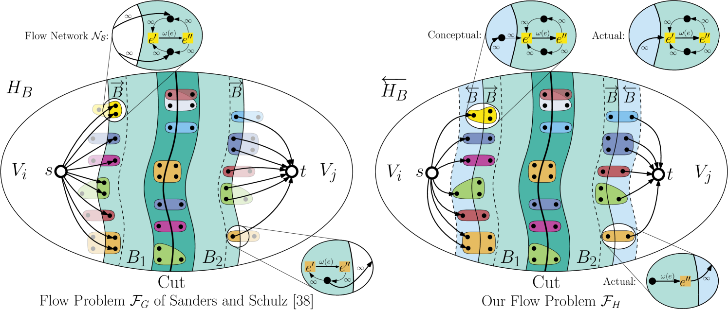
3.2. Constructing the Hypergraph Flow Problem
Let be the subhypergraph of that is induced by a corridor computed in the bipartition . In the following, we distinguish between the set of internal border nodes and the set of external border nodes . Similarly, we distinguish between external nets with no pins inside , internal nets with all pins inside , and border nets with some pins inside and some pins outside of . We use to denote the set of border nets.
A hypergraph flow problem consists of a flow network derived from and two additional nodes and that are connected to some nodes . Our approach works with all flow networks presented in Section 3.1. A flow problem has the cut property if the resulting min-cut bipartition of does not increase the -metric in . Thus it has to hold that . While external nets are not affected by a max-flow computation, the max-flow min-cut theorem [21] ensures the cut property for all internal nets. Border nets however require special attention. Since a border net is only partially contained in , it will remain connected to the blocks of its external border nodes in . In case external border nodes connect to both and , it will remain a cut net in even if it is removed from the cut-set in . It is therefore necessary to “encode” information about external border nodes into the flow problem.
The KaFFPa Model and its Limitations.
In KaFFPa, this is done by directly connecting internal border nodes to and . This approach can also be used for hypergraphs. In the hypergraph flow problem , the source is connected to all nodes and all nodes are connected to using directed edges with infinite capacity. While this ensures that has the cut property, applying the graph-based model to hypergraphs unnecessarily restricts the search space. Since all internal border nodes are connected to either or , every min-cut will have and . The KaFFPa model therefore prevents all min-cuts in which any non-cut border net (i.e., with ) becomes part of the cut-set. This restricts the space of possible solutions, since corridor was computed such that even a min-cut along either side of the border would result in a feasible cut in . Thus, ideally, all vertices should be able to change their block as result of an -max-flow computation on – not only vertices . This limitation becomes increasingly relevant for hypergraphs with large nets as well as for partitioning problems with small imbalance , since large nets are likely to be only partially contained in and tight balance constraints enforce small -corridors. While the former is a problem only for HGP, the latter also applies to GP.
A more flexible Model.
We propose a more general model that allows an -max-flow computation to also cut through border nets by exploiting the structure of hypergraph flow networks. Instead of directly connecting and to internal border nodes and thus preventing all min-cuts in which these nodes switch blocks, we conceptually extend to contain all external border nodes and all border nets . The resulting hypergraph is . The key insight now is that by using the flow network of and connecting resp. to the external border nodes resp. , we get a flow problem that does not lock any node in its block, since none of these nodes is directly connected to either or . Due to the max-flow min-cut theorem [21], this flow problem furthermore has the cut property, since all border nets of are now internal nets and all external border nodes are locked inside their block. However, it is not necessary to use instead of to achieve this result. For all vertices the flow network of contains paths and that only involve infinite-capacity edges. Therefore we can remove all nodes by directly connecting and to the corresponding bridging nodes via infinite-capacity edges without affecting the maximal flow [20]. More precisely, in the hypergraph flow problem , we connect to all bridging nodes corresponding to border nets and all bridging nodes corresponding to border nets to using directed, infinite-capacity edges.
Single-Pin Border Nets.
Furthermore, we model border nets with more efficiently. For such a net , the flow problem contains paths of the form or which can be replaced by paths of the form or with resp. . In both cases we can thus remove one bridging node and two infinite-capacity edges. A comparison of and is shown in Figure 2.
3.3. Implementation Details
Since KaHyPar is an -level partitioner, its FM-based local search algorithms are executed each time a vertex is uncontracted. To prevent expensive recalculations, it therefore uses a cache to maintain the gain values of FM moves throughout the -level hierarchy [2]. In order to combine our flow-based refinement with FM local search, we not only perform the moves induced by the max-flow min-cut computation but also update the FM gain cache accordingly.
Since it is not feasible to execute our algorithm on every level of the -level hierarchy, we use an exponentially spaced approach that performs flow-based refinements after uncontracting vertices for . This way, the algorithm is executed more often on smaller flow problems than on larger ones. To further improve the running time, we introduce the following speedup techniques:
-
•
S1: We modify active block scheduling such that after the first round the algorithm is only executed on a pair of blocks if at least one execution using these blocks improved connectivity or imbalance of the partition on previous levels.
-
•
S2: For all levels except the finest level: Skip flow-based refinement if the cut between two adjacent blocks is less than ten.
-
•
S3: Stop resizing the corridor if the current -cut did not improve the previously best solution.
4. Experimental Evaluation
We implemented the max-flow min-cut refinement algorithm in the -level hypergraph partitioning framework KaHyPar (Karlsruhe Hypergraph Partitioning). The code is written in C++ and compiled using g++-5.2 with flags -O3 -march=native. The latest version of the framework is called KaHyPar-CA [28]. We refer to our new algorithm as KaHyPar-MF. Both versions use the default configuration for community-aware direct -way partitioning.111https://github.com/SebastianSchlag/kahypar/blob/master/config/km1_direct_kway_sea17.ini
Instances.
All experiments use hypergraphs from the benchmark set of Heuer and Schlag [28]222The complete benchmark set along with detailed statistics for each hypergraph is publicly available from http://algo2.iti.kit.edu/schlag/sea2017/., which contains hypergraphs derived from four benchmark sets: the ISPD98 VLSI Circuit Benchmark Suite [3], the DAC 2012 Routability-Driven Placement Contest [55], the University of Florida Sparse Matrix Collection [15], and the international SAT Competition 2014 [9]. Sparse matrices are translated into hypergraphs using the row-net model [12], i.e., each row is treated as a net and each column as a vertex. SAT instances are converted to three different representations: For literal hypergraphs, each boolean literal is mapped to one vertex and each clause constitutes a net [43], while in the primal model each variable is represented by a vertex and each clause is represented by a net. In the dual model the opposite is the case [41]. All hypergraphs have unit vertex and net weights.
Table 1 gives an overview about the different benchmark sets used in the experiments. The full benchmark set is referred to as set A. We furthermore use the representative subset of 165 hypergraphs proposed in [28] (set B) and a smaller subset consisting of hypergraphs (set C), which is used to devise the final configuration of KaHyPar-MF. Basic properties of set C can be found in Table 10 in Appendix C. Unless mentioned otherwise, all hypergraphs are partitioned into blocks with . For each value of , a -way partition is considered to be one test instance, resulting in a total of instances for set C, instances for set B and instances for set A. Furthermore we use 15 graphs from [42] to compare our flow model to the KaFFPa [47] model . Table 11 in Appendix C summarizes the basic properties of these graphs, which constitute set D.
System and Methodology.
All experiments are performed on a single core of a machine consisting of two Intel Xeon E5-2670 Octa-Core processors (Sandy Bridge) clocked at GHz. The machine has GB main memory, MB L3- and 8x256 KB L2-Cache and is running RHEL 7.2. We compare KaHyPar-MF to KaHyPar-CA, as well as to the -way (hMetis-K) and the recursive bisection variant (hMetis-R) of hMetis 2.0 (p1) [32, 33], and to PaToH 3.2 [12]. These HGP libraries were chosen because they provide the best solution quality [2, 28]. The partitioning results of these tools are already available from http://algo2.iti.kit.edu/schlag/sea2017/. For each partitioner except PaToH the results summarize ten repetitions with different seeds for each test instance and report the arithmetic mean of the computed cut and running time as well as the best cut found. Since PaToH ignores the random seed if configured to use the quality preset, the results contain both the result of single run of the quality preset (PaToH-Q) and the average over ten repetitions using the default configuration (PaToH-D). Each partitioner had a time limit of eight hours per test instance. We use the same number of repetitions and the same time limit for our experiments with KaHyPar-MF.
In the following, we use the geometric mean when averaging over different instances in order to give every instance a comparable influence on the final result. In order to compare the algorithms in terms of solution quality, we perform a more detailed analysis using improvement plots. For each algorithm, these plots relate the minimum connectivity of KaHyPar-MF to the minimum connectivity produced by the corresponding algorithm on a per-instance basis. For each algorithm, these ratios are sorted in decreasing order. The plots use a cube root scale for the y-axis to reduce right skewness [14] and show the improvement of KaHyPar-MF in percent (i.e., ) on the y-axis. A value below zero indicates that the partition of KaHyPar-MF was worse than the partition produced by the corresponding algorithm, while a value above zero indicates that KaHypar-MF performed better than the algorithm in question. A value of zero implies that the partitions of both algorithms had the same solution quality. Values above one correspond to infeasible solutions that violated the balance constraint. In order to include instances with a cut of zero into the results, we set the corresponding cut values to one for ratio computations.
| Type | # | ||||
|---|---|---|---|---|---|
| DAC | 5 | 3.32 | 3.28 | 3.37 | 3.35 |
| ISPD | 10 | 4.20 | 4.24 | 3.89 | 3.90 |
| Primal | 30 | 16.29 | 9.97 | 2.63 | 2.39 |
| Literal | 30 | 8.21 | 4.99 | 2.63 | 2.39 |
| Dual | 30 | 2.63 | 2.38 | 16.29 | 9.97 |
| SPM | 60 | 24.78 | 14.15 | 26.58 | 15.01 |
4.1. Evaluating Flow Networks, Models, and Algorithms
Flow Networks and Algorithms.
To analyze the effects of the different hypergraph flow networks we compute five bipartitions for each hypergraph of set B with KaHyPar-CA using different seeds. Statistics of the hypergraphs are shown in Table 2. The bipartitions are then used to generate hypergraph flow networks for a corridor of size hypernodes around the cut. Figure 3 (top) summarizes the sizes of the respective flow networks in terms of number of nodes and number of edges for each instance class. The flow networks of primal and literal SAT instances are the largest in terms of both numbers of nodes and edges. High average vertex degree combined with low average net sizes leads to subhypergraphs containing many small nets, which then induce many nodes and (infinite-capacity) edges in . Dual instances with low average degree and large average net size on the other hand lead to smaller flow networks. For VLSI instances (DAC, ISPD) both average degree and average net sizes are low, while for SPM hypergraphs the opposite is the case. This explains why SPM flow networks have significantly more edges, despite the number of nodes being comparable in both classes.
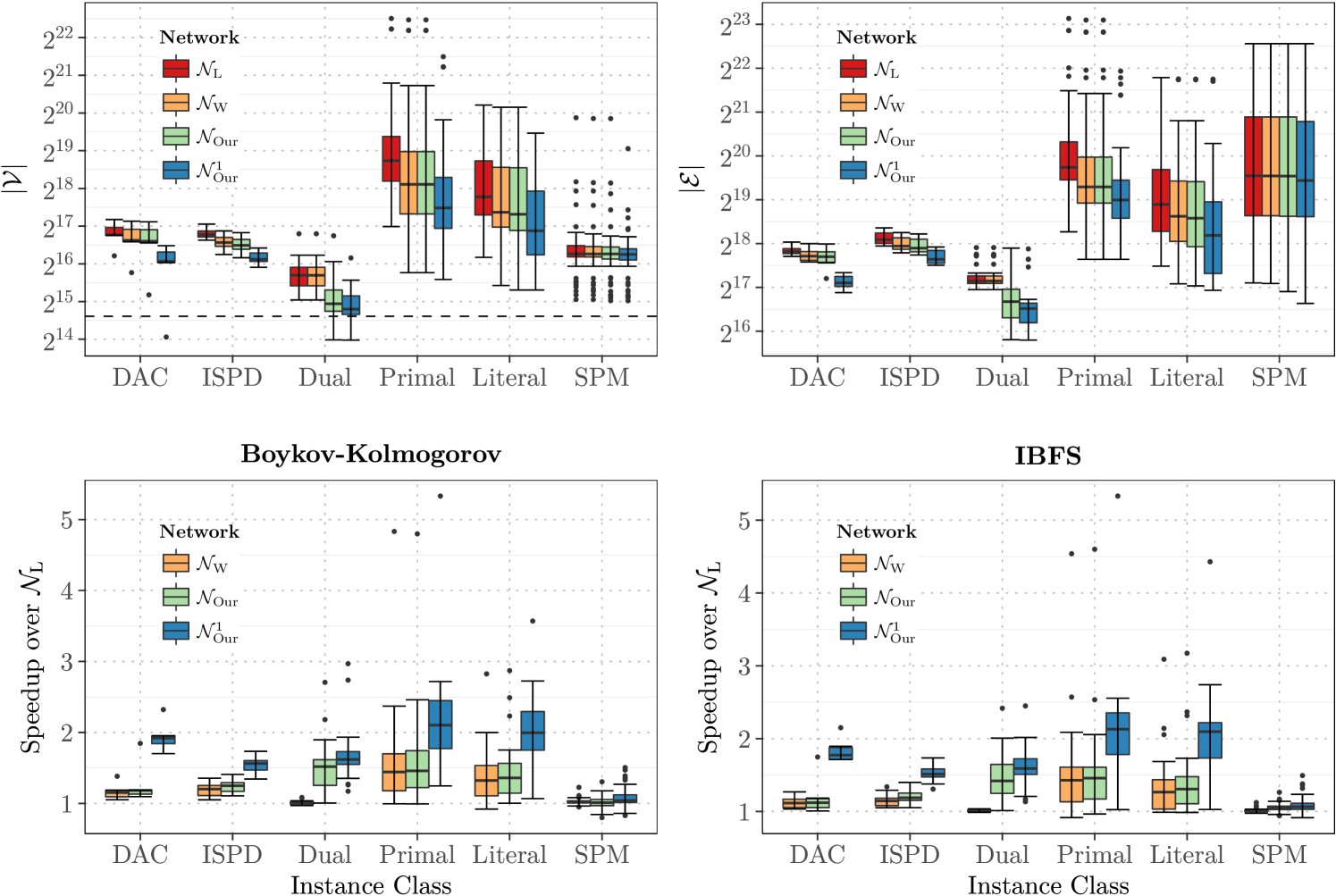
As expected, the Lawler-Network induces the biggest flow problems. Looking at the Liu-Wong network , we can see that distinguishing between graph edges and nets with pins has an effect for all hypergraphs with many small nets (i.e., DAC, ISPD, Primal, Literal). While this technique alone does not improve dual SAT instances, we see that the combination of the Liu-Wong approach and our removal of low degree hypernodes in reduces the size of the networks for all instance classes except SPM. Both techniques only have a limited effect on these instances, since both hypernode degrees and net sizes are large on average. Since our flow problems are based on -corridor induced subhypergraphs, additionally models single-pin border nets more efficiently as described in Section 3.2. This further reduces the network sizes significantly. As expected, the reduction in numbers of nodes and edges is most pronounced for hypergraphs with low average net sizes because these instances are likely to contain many single-pin border nets.
To further see how these reductions in network size translate to improved running times of max-flow algorithms, we use these networks to create flow problems using our flow model and compute min-cuts using two highly tuned max-flow algorithms, namely the BK-algorithm333Available from: https://github.com/gerddie/maxflow [10] and the incremental breadth-first search (IBFS) algorithm444Available from: http://www.cs.tau.ac.il/~sagihed/ibfs/code.html [23]. These algorithms were chosen because they performed best in preliminary experiments [27]. We then compare the speedups of these algorithms when executed on , , and to the execution on the Lawler network . As can be seen in Figure 3 (bottom) both algorithms benefit from improved network models and the speedups directly correlate with the reductions in network size. While significantly reduces the running times for Primal and Literal instances, additionally leads to a speedup for Dual instances. By additionally considering single-pin border nets, results in an average speedup between and (except for SPM instances). Since IBFS outperformed the BK algorithm in [27], we use and IBFS in all following experiments.
| Hypergraphs | Graphs | |||||
Flow Models.
We now compare the flow model of KaFFPa to our advanced model described in Section 3.2. The experiments summarized in Table 4.1 were performed using sets C and D. To focus on the impact of the models on solution quality, we deactivated KaHyPar’s FM local search algorithms and only use flow-based refinement without the most balanced minimum cut heuristic. The results confirm our hypothesis that restricts the space of possible solutions. For all flow problem sizes and all imbalances tested, yields better solution quality. As expected, the effects are most pronounced for small flow problems and small imbalances where many vertices are likely to be border nodes. Since these nodes are locked inside their respective block in , they prevent all non-cut border nets from becoming part of the cut-set. Our model, on the other hand, allows all min-cuts that yield a feasible solution for the original partitioning problem. The fact that this effect also occurs for the graphs of set D indicates that our model can also be effective for traditional graph partitioning. All following experiments are performed using .
4.2. Configuring the Algorithm
We now evaluate different configurations of the max-flow min-cut based refinement framework on set C. In the following, KaHyPar-CA [28] is used as a reference. Since it neither uses (F)lows nor the (M)ost balanced minimum cut heuristic and only relies on the (FM) algorithm for local search, it is referred to as (-F,-M,+FM). This basic configuration is then successively extended with specific components. The results of our experiments are summarized in Table 4.2 for increasing scaling parameter . The table furthermore includes a configuration Constant128. In this configuration all components are enabled (+F,+M,+FM) and we perform flow-based refinements every 128 uncontractions. While this configuration is slow, it is used as a reference point for the quality achievable using flow-based refinement.
The results indicate that only using flows (+F,-M,-FM) as refinement technique is inferior to localized FM local search in regard to both running time and solution quality. Although the quality improves with increasing flow problem size (i.e., increasing ), the average connectivity is still worse than the reference configuration. Enabling the most balanced minimum cut heuristic improves partitioning quality. Configuration (+F,+M,-FM) performs better than the basic configuration for . By combining flows with the FM algorithm (+F,-M,+FM) we get a configuration that improves upon the baseline configuration even for small flow problems. However, comparing this variant with (+F,+M,-FM) for , we see that using large flow problems together with the most balanced minimum cut heuristic yields solutions of comparable quality. Enabling all components (+F,+M,+FM) and using large flow problems performs best. Furthermore we see that enabling FM local search slightly improves the running time for . This can be explained by the fact that the FM algorithm already produces good cuts between the blocks such that fewer rounds of pairwise flow refinements are necessary to further improve the solution. Comparing configuration (+F,+M,+FM) with Constant128 shows that performing flows more often further improves solution quality at the cost of slowing down the algorithm by more than an order of magnitude. In all further experiments, we therefore use configuration (+F,+M,+FM) with for KaHyPar-MF. This configuration also performed best in the effectiveness tests presented in Appendix A. While this configuration performs better than KaHyPar-CA, its running time is still more than a factor of higher.
We therefore perform additional experiments on set B and successively enable the speedup heuristics described in Section 3.3. The results are summarized in Table 4.2. Only executing pairwise flow refinements on blocks that lead to an improvement on previous levels (S1) reduces the running time of flow-based refinement by a factor of , while skipping flows in case of small cuts (S2) results in a further speedup of . By additionally stopping the resizing of the flow problem as early as possible (S3), we decrease the running time of flow-based improvement by a factor of in total, while still computing solutions of comparable quality. Thus in the comparisons with other systems, all heuristics are enabled.
4.3. Comparison with other Systems
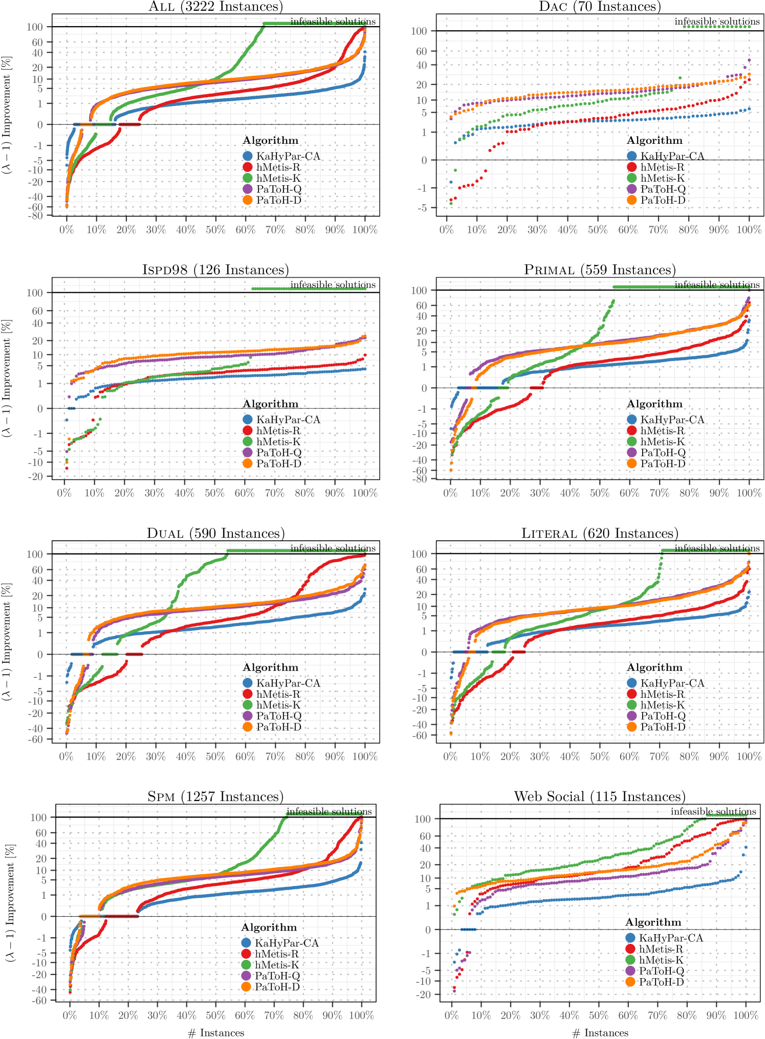
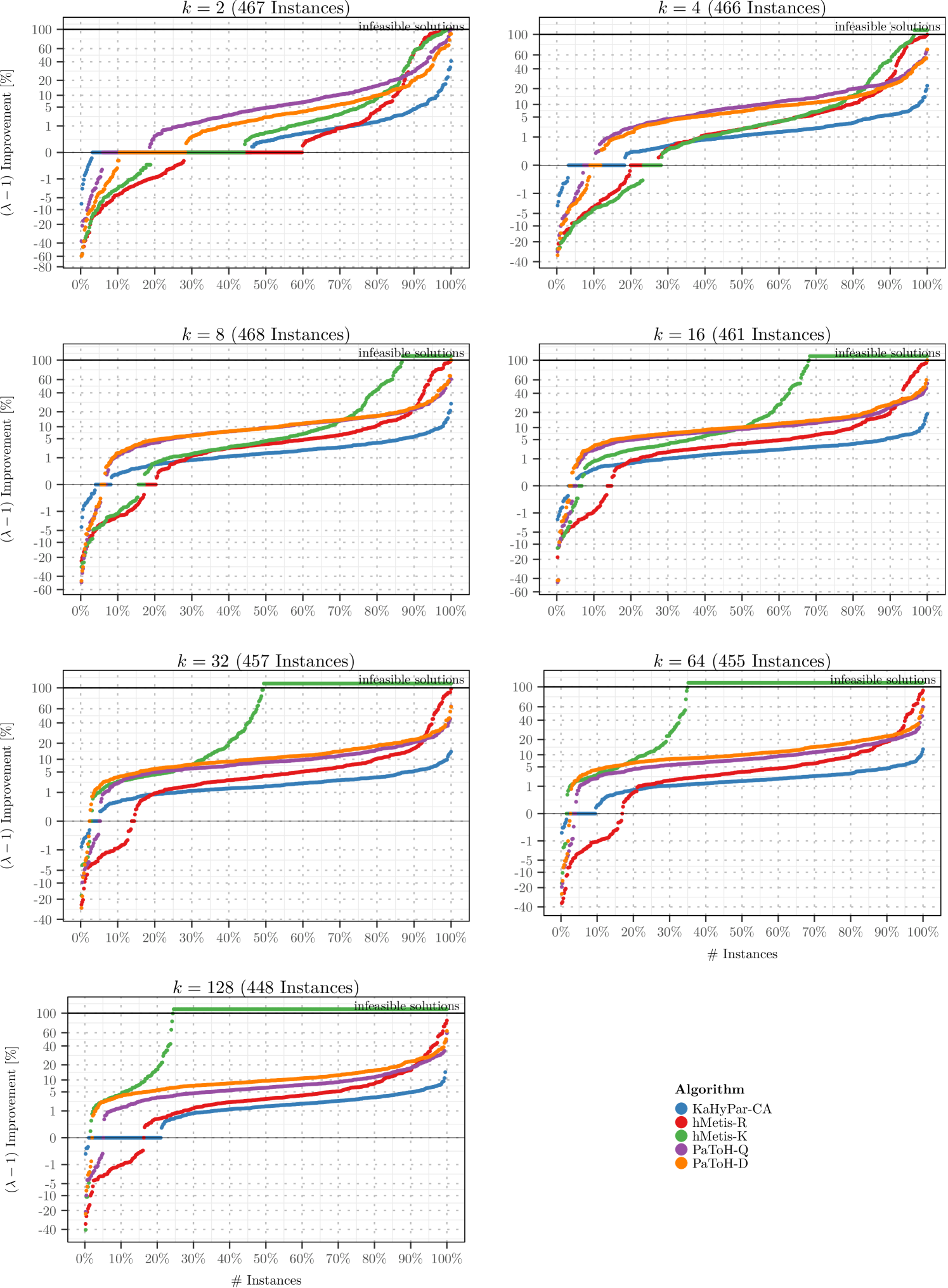
Finally, we compare KaHyPar-MF to different state-of-the-art hypergraph partitioners on the full benchmark set. We exclude the same out of instances as in [28] because either PaToH-Q could not allocate enough memory or other partitioners did not finish in time. The excluded instances are shown in Table LABEL:tbl:excluded in Appendix D. Note that KaHyPar-MF did not lead to any further exclusions. The following comparison is therefore based on the remaining 3222 instances. As can be seen in Figure 4, KaHyPar-MF outperforms all other algorithms on all benchmark sets. Comparing the best solutions of KaHyPar-MF to each partitioner individually across all instances (top left), KaHyPar-MF produced better partitions than PaToH-Q, PaToH-D, hMetis-K, KaHyPar-CA, hMetis-R for , , , , and of the instances, respectively.
Comparing the best solutions of all systems simultaneously, KaHyPar-MF produced the best partitions for of the instances. It is followed by hMetis-R (), KaHyPar-CA (), hMetis-K (), PaToH-D (), and PaToH-Q (). Note that for some instances multiple partitioners computed the same best solution and that we disqualified infeasible solutions that violated the balance constraint.
Figure 5 shows that KaHyPar-MF also performs best for different values of and that pairwise flow refinements are an effective strategy to improve -way partitions. As can be seen in Table 4.3, the improvement over KaHyPar-CA is most pronounced for hypergraphs derived from matrices of web graphs and social networks555Based on the following matrices: webbase-1M, ca-CondMat, soc-sign-epinions, wb-edu, IMDB, as-22july06, as-caida, astro-ph, HEP-th, Oregon-1, Reuters911, PGPgiantcompo, NotreDame_www, NotreDame_actors, p2p-Gnutella25, Stanford, cnr-2000. and dual SAT instances. While the former are difficult to partition due to skewed degree and net size distributions, the latter are difficult because they contain many large nets.
Finally, Table B compares the running times of all partitioners. By using simplified flow networks, highly tuned flow algorithms and several techniques to speed up the flow-based refinement framework, KaHyPar-MF is less than a factor of two slower than KaHyPar-CA and still achieves a running time comparable to that of hMetis.
KaHyPar-MF 1005.76 2985.22 5805.19 9097.31 14352.34 21537.33 31312.48 KaHyPar-CA 1.71 2.16 2.51 2.51 2.45 2.16 2.05 hMetis-R 22.25 17.62 15.63 14.29 11.94 9.80 8.01 hMetis-K 21.82 13.66 12.76 13.49 10.62 9.18 7.81 PaToH-Q 14.92 12.60 11.81 11.66 10.66 9.77 8.63 PaToH-D 8.54 10.41 13.64 14.50 12.70 12.66 11.89
KaHyPar-MF 19.75 32.89 47.52 60.38 78.51 100.34 119.15 KaHyPar-CA 12.68 17.16 23.88 31.01 41.69 57.35 76.61 hMetis-R 27.87 51.59 74.74 91.09 109.13 128.66 149.34 hMetis-K 25.47 32.27 42.50 53.41 74.00 109.12 152.92 PaToH-Q 1.93 3.61 5.44 7.01 8.40 10.06 11.44 PaToH-D 0.43 0.77 1.12 1.42 1.71 2.02 2.29
5. Conclusion
We generalize the flow-based refinement framework of KaFFPa [47] from graph to hypergraph partitioning. We reduce the size of Liu and Wong’s hypergraph flow network [40] by removing low degree hypernodes and exploiting the fact that our flow problems are built on subhypergraphs of the input hypergraph. Furthermore we identify shortcomings of the KaFFPa [47] approach that restrict the search space of feasible solutions significantly and introduce an advanced model that overcomes these limitations by exploiting the structure of hypergraph flow networks. Lastly, we present techniques to improve the running time of the flow-based refinement framework by a factor of without affecting solution quality. The resulting hypergraph partitioner KaHyPar-MF performs better than all competing algorithms on all instance classes of a large benchmark set and still has a running time comparable to that of hMetis.
Since our flow problem formulation yields significantly better solutions for both hypergraphs and graphs than the KaFFPa [47] approach, future work includes the integration of our flow model into KaFFPa and the evaluation in the context of a high quality graph partitioner. Furthermore an approach similar to Yang and Wong [57] could be used as an alternative to the most balanced minimum cut heuristic and adaptive -corridor resizing. We also plan to extend our framework to optimize other objective functions such as cut or sum of external degrees.
References
- [1] P. Agrawal, B. Narendran, and N. Shivakumar. Multi-way partitioning of VLSI circuits. In Proceedings of 9th International Conference on VLSI Design, pages 393–399, Jan 1996.
- [2] Y. Akhremtsev, T. Heuer, P. Sanders, and S. Schlag. Engineering a direct k-way hypergraph partitioning algorithm. In 19th Workshop on Algorithm Engineering and Experiments, (ALENEX), pages 28–42, 2017.
- [3] C. J. Alpert. The ISPD98 Circuit Benchmark Suite. In Proceedings of the 1998 International Symposium on Physical Design, pages 80–85. ACM, 1998.
- [4] C. J. Alpert, J.-H. Huang, and A. B. Kahng. Multilevel Circuit Partitioning. IEEE Transactions on Computer-Aided Design of Integrated Circuits and Systems, 17(8):655–667, 1998.
- [5] C. J. Alpert and A. B. Kahng. Recent Directions in Netlist Partitioning: a Survey. Integration, the VLSI Journal, 19(1–2):1 – 81, 1995.
- [6] Reid Andersen and Kevin J Lang. An Algorithm for Improving Graph Partitions. In Proceedings of the 19th annual ACM-SIAM Symposium on Discrete Algorithms, pages 651–660. Society for Industrial and Applied Mathematics, 2008.
- [7] C. Aykanat, B. B. Cambazoglu, and B. Uçar. Multi-level Direct K-way Hypergraph Partitioning with Multiple Constraints and Fixed Vertices. Journal of Parallel and Distributed Computing, 68(5):609–625, 2008.
- [8] D. A. Bader, H. Meyerhenke, P. Sanders, and D. Wagner, editors. Proc. Graph Partitioning and Graph Clustering - 10th DIMACS Implementation Challenge Workshop, volume 588 of Contemporary Mathematics. AMS, 2013.
- [9] A. Belov, D. Diepold, M. Heule, and M. Järvisalo. The SAT Competition 2014. http://www.satcompetition.org/2014/, 2014.
- [10] Yuri Boykov and Vladimir Kolmogorov. An Experimental Comparison of Min-Cut/Max-Flow Algorithms for Energy Minimization in Vision. IEEE Transactions on Pattern Analysis and Machine Intelligence, 26(9):1124–1137, 2004.
- [11] T. N. Bui and C. Jones. A Heuristic for Reducing Fill-In in Sparse Matrix Factorization. In SIAM Conference on Parallel Processing for Scientific Computing, pages 445–452, 1993.
- [12] Ü. V. Catalyürek and C. Aykanat. Hypergraph-Partitioning-Based Decomposition for Parallel Sparse-Matrix Vector Multiplication. IEEE Transactions on Parallel and Distributed Systems, 10(7):673–693, Jul 1999.
- [13] J. Cong and M. Smith. A Parallel Bottom-up Clustering Algorithm with Applications to Circuit Partitioning in VLSI Design. In 30th Conference on Design Automation, pages 755–760, June 1993.
- [14] N. J. Cox. Stata tip 96: Cube roots. Stata Journal, 11(1):149–154(6), 2011. URL: http://www.stata-journal.com/article.html?article=st0223.
- [15] T. A. Davis and Y. Hu. The University of Florida Sparse Matrix Collection. ACM Transactions on Mathematical Software, 38(1):1:1–1:25, 2011.
- [16] K. D. Devine, E. G. Boman, R. T. Heaphy, R. H. Bisseling, and Ü. V. Catalyürek. Parallel Hypergraph Partitioning for Scientific Computing. In 20th International Conference on Parallel and Distributed Processing, IPDPS, pages 124–124. IEEE, 2006.
- [17] W.E. Donath. Logic partitioning. Physical Design Automation of VLSI Systems, pages 65–86, 1988.
- [18] J. Edmonds and R. M. Karp. Theoretical Improvements in Algorithmic Efficiency for Network Flow Problems. Journal of the ACM, 19(2):248–264, 1972.
- [19] C. Fiduccia and R. Mattheyses. A Linear Time Heuristic for Improving Network Partitions. In 19th ACM/IEEE Design Automation Conf., pages 175–181, 1982.
- [20] D. R. Ford and D. R. Fulkerson. Flows in Networks. Princeton University Press, 1962.
- [21] Lester R Ford and Delbert R Fulkerson. Maximal Flow through a Network. Canadian Journal of Mathematics, 8(3):399–404, 1956.
- [22] A. V. Goldberg and R. E. Tarjan. A new approach to the maximum-flow problem. Journal of the ACM, 35(4):921–940, 1988.
- [23] Andrew Goldberg, Sagi Hed, Haim Kaplan, Robert Tarjan, and Renato Werneck. Maximum Flows by Incremental Breadth-First Search. Proceedings of 2011 European Symposium on Algorithms, pages 457–468, 2011.
- [24] M. Hamann and B. Strasser. Graph Bisection with Pareto-Optimization. In Proceedings of the Eighteenth Workshop on Algorithm Engineering and Experiments, ALENEX 2016, Arlington, Virginia, USA, January 10, 2016, pages 90–102, 2016.
- [25] S. Hauck and G. Borriello. An Evaluation of Bipartitioning Techniques. IEEE Transactions on Computer-Aided Design of Integrated Circuits and Systems, 16(8):849–866, Aug 1997.
- [26] B. Hendrickson and R. Leland. A Multi-Level Algorithm For Partitioning Graphs. SC Conference, 0:28, 1995.
- [27] T. Heuer. High Quality Hypergraph Partitioning via Max-Flow-Min-Cut Computations. Master’s thesis, KIT, 2018.
- [28] T. Heuer and S. Schlag. Improving Coarsening Schemes for Hypergraph Partitioning by Exploiting Community Structure. In 16th International Symposium on Experimental Algorithms, (SEA), page 21:1–21:19, 2017.
- [29] T. C. Hu and K. Moerder. Multiterminal Flows in a Hypergraph. In T.C. Hu and E.S. Kuh, editors, VLSI Circuit Layout: Theory and Design, chapter 3, pages 87–93. IEEE Press, 1985.
- [30] E. Ihler, D. Wagner, and F. Wagner. Modeling Hypergraphs by Graphs with the Same Mincut Properties. Inf. Process. Lett., 45(4):171–175, 1993.
- [31] I. Kabiljo, B. Karrer, M. Pundir, S. Pupyrev, A. Shalita, Y. Akhremtsev, and Presta. A. Social Hash Partitioner: A Scalable Distributed Hypergraph Partitioner. PVLDB, 10(11):1418–1429, 2017.
- [32] G. Karypis, R. Aggarwal, V. Kumar, and S. Shekhar. Multilevel Hypergraph Partitioning: Applications in VLSI Domain. IEEE Transactions on Very Large Scale Integration VLSI Systems, 7(1):69–79, 1999.
- [33] G. Karypis and V. Kumar. Multilevel -way Hypergraph Partitioning. In Proceedings of the 36th ACM/IEEE Design Automation Conference, pages 343–348. ACM, 1999.
- [34] B. W. Kernighan and S. Lin. An Efficient Heuristic Procedure for Partitioning Graphs. The Bell System Technical Journal, 49(2):291–307, Feb 1970.
- [35] K. Lang and S. Rao. A Flow-Based Method for Improving the Expansion or Conductance of Graph Cuts. In Proceedings of 10th International IPCO Conference, volume 4, pages 325–337. Springer, 2004.
- [36] E. Lawler. Cutsets and Partitions of Hypergraphs. Networks, 3(3):275–285, 1973.
- [37] E. Lawler. Combinatorial Optimization : Networks and Matroids. Holt, Rinehart, and Whinston, 1976.
- [38] T. Lengauer. Combinatorial Algorithms for Integrated Circuit Layout. John Wiley & Sons, Inc., 1990.
- [39] J. Li, J. Lillis, and C. K. Cheng. Linear decomposition algorithm for VLSI design applications. In Proceedings of IEEE International Conference on Computer Aided Design (ICCAD), pages 223–228, Nov 1995.
- [40] H. Liu and D. F. Wong. Network-Flow-Based Multiway Partitioning with Area and Pin Constraints. IEEE Transactions on Computer-Aided Design of Integrated Circuits and Systems, 17(1):50–59, Jan 1998.
- [41] Z. Mann and P. Papp. Formula partitioning revisited. In Daniel Le Berre, editor, POS-14. Fifth Pragmatics of SAT workshop, volume 27 of EPiC Series in Computing, pages 41–56. EasyChair, 2014.
- [42] H. Meyerhenke, P. Sanders, and C. Schulz. Partitioning Complex Networks via Size-Constrained Clustering. In 13th International Symposium on Experimental Algorithms, (SEA), pages 351–363, 2014.
- [43] D. A. Papa and I. L. Markov. Hypergraph Partitioning and Clustering. In T. F. Gonzalez, editor, Handbook of Approximation Algorithms and Metaheuristics. Chapman and Hall/CRC, 2007.
- [44] Jean-Claude Picard and Maurice Queyranne. On the Structure of all Minimum Cuts in a Network and Applications. Combinatorial Optimization II, pages 8–16, 1980.
- [45] Joachim Pistorius and Michel Minoux. An Improved Direct Labeling Method for the Max–Flow Min–Cut Computation in Large Hypergraphs and Applications. International Transactions in Operational Research, 10(1):1–11, 2003.
- [46] L. A. Sanchis. Multiple-way Network Partitioning. IEEE Trans. on Computers, 38(1):62–81, 1989. doi:10.1109/12.8730.
- [47] P. Sanders and C. Schulz. Engineering Multilevel Graph Partitioning Algorithms. In 19th European Symposium on Algorithms, volume 6942 of LNCS, pages 469–480. Springer, 2011.
- [48] S. Schlag, V. Henne, T. Heuer, H. Meyerhenke, P. Sanders, and C. Schulz. -way Hypergraph Partitioning via -Level Recursive Bisection. In 18th Workshop on Algorithm Engineering and Experiments (ALENEX), pages 53–67, 2016.
- [49] D. G. Schweikert and B. W. Kernighan. A Proper Model for the Partitioning of Electrical Circuits. In Proceedings of the 9th Design Automation Workshop, DAC, pages 57–62. ACM, 1972.
- [50] A. Trifunovic. Parallel Algorithms for Hypergraph Partitioning. PhD thesis, University of London, 2006.
- [51] A. Trifunović and W. J. Knottenbelt. Parallel Multilevel Algorithms for Hypergraph Partitioning. Journal of Parallel and Distributed Computing, 68(5):563 – 581, 2008.
- [52] Ü. V. Çatalyürek and M. Deveci and K. Kaya and B. Uçar. UMPa: A multi-objective, multi-level partitioner for communication minimization. In Bader et al. [8], pages 53–66.
- [53] B. Uçar and C. Aykanat. Encapsulating Multiple Communication-Cost Metrics in Partitioning Sparse Rectangular Matrices for Parallel Matrix-Vector Multiplies. SIAM Journal on Scientific Computing, 25(6):1837–1859, 2004.
- [54] B. Vastenhouw and R. H. Bisseling. A Two-Dimensional Data Distribution Method for Parallel Sparse Matrix-Vector Multiplication. SIAM Review, 47(1):67–95, 2005.
- [55] N. Viswanathan, C. Alpert, C. Sze, Z. Li, and Y. Wei. The dac 2012 routability-driven placement contest and benchmark suite. In Proceedings of the 49th Annual Design Automation Conference, DAC ’12, pages 774–782. ACM, 2012.
- [56] S. Wichlund. On multilevel circuit partitioning. In 1998 International Conference on Computer-aided Design, ICCAD, pages 505–511. ACM, 1998.
- [57] H. H. Yang and D. F. Wong. Efficient Network Flow Based Min-Cut Balanced Partitioning. IEEE Transactions on Computer-Aided Design of Integrated Circuits and Systems, 15(12):1533–1540, 1996.
Appendix A Effectiveness Tests
To evaluate the effectiveness of our configurations presented in Section 4.2 we give each configuration the same time to compute a partition. For each instance (hypergraph, ), we execute each configuration once and note the largest running time . Then each configuration gets time to compute a partition (i.e., we take the best partition out of several repeated runs). Whenever a new run of a partition would exceed the largest running time, we perform the next run with a certain probability such that the expected running time is . The results of this procedure, which was initially proposed in [47], are presented in Table A. We see that the combinations of flow-based refinement and FM local search perform better than repeated executions of the baseline configuration (-F,-M,+FM). The most effective configuration is (+F,+M,-FM) with , which was chosen as the default configuration for KaHyPar-MF.
Appendix B Average Connectivity Improvement
KaHyPar-MF 1057.93 3130.20 6032.58 9362.55 14693.96 21893.59 31706.57 KaHyPar-CA 2.27 2.57 2.80 2.68 2.48 2.24 2.05 hMetis-R 21.38 15.92 14.47 13.63 11.35 9.63 7.80 hMetis-K 21.63 15.15 13.61 13.49 10.52 9.30 7.83 PaToH-Q 10.51 8.36 8.35 9.09 8.54 8.27 7.48 PaToH-D 13.26 14.24 16.07 16.59 13.87 13.61 12.66
Appendix C Properties of Benchmark Sets
| Class | Hypergraph | |||
|---|---|---|---|---|
| ISPD | ibm06 | 32 498 | 34 826 | 128 182 |
| ibm07 | 45 926 | 48 117 | 175 639 | |
| ibm08 | 51 309 | 50 513 | 204 890 | |
| ibm09 | 53 395 | 60 902 | 222 088 | |
| ibm10 | 69 429 | 75 196 | 297 567 | |
| Dual | 6s9 | 100 384 | 34 317 | 234 228 |
| 6s133 | 140 968 | 48 215 | 328 924 | |
| 6s153 | 245 440 | 85 646 | 572 692 | |
| dated-10-11-u | 629 461 | 141 860 | 1 429 872 | |
| dated-10-17-u | 1 070 757 | 229 544 | 2 471 122 | |
| Literal | 6s133 | 96 430 | 140 968 | 328 924 |
| 6s153 | 171 292 | 245 440 | 572 692 | |
| aaai10-planning-ipc5 | 107 838 | 308 235 | 690 466 | |
| dated-10-11-u | 283 720 | 629 461 | 1 429 872 | |
| atco_enc2_opt1_05_21 | 112 732 | 526 872 | 2 097 393 | |
| Primal | 6s153 | 85 646 | 245 440 | 572 692 |
| aaai10-planning-ipc5 | 53 919 | 308 235 | 690 466 | |
| hwmcc10-timeframe | 163 622 | 488 120 | 1 138 944 | |
| dated-10-11-u | 141 860 | 629 461 | 1 429 872 | |
| atco_enc2_opt1_05_21 | 56 533 | 526 872 | 2 097 393 | |
| SPM | mult_dcop_01 | 25 187 | 25 187 | 193 276 |
| vibrobox | 12 328 | 12 328 | 342 828 | |
| RFdevice | 74 104 | 74 104 | 365 580 | |
| mixtank_new | 29 957 | 29 957 | 1 995 041 | |
| laminar_duct3D | 67 173 | 67 173 | 3 833 077 |
| Graph | ||
|---|---|---|
| p2p-Gnutella04 | 6 405 | 29 215 |
| wordassociation-2011 | 10 617 | 63 788 |
| PGPgiantcompo | 10 680 | 24 316 |
| email-EuAll | 16 805 | 60 260 |
| as-22july06 | 22 963 | 48 436 |
| soc-Slashdot0902 | 28 550 | 379 445 |
| loc-brightkite | 56 739 | 212 945 |
| enron | 69 244 | 254 449 |
| loc-gowalla | 196 591 | 950 327 |
| coAuthorsCiteseer | 227 320 | 814 134 |
| wiki-Talk | 232 314 | 1.5M |
| citationCiteseer | 268 495 | 1.2M |
| coAuthorsDBLP | 299 067 | 977 676 |
| cnr-2000 | 325 557 | 2.7M |
| web-Google | 356 648 | 2.1M |
Appendix D Excluded Instances
| Hypergraph | 2 | 4 | 8 | 16 | 32 | 64 | 128 |
| Primal | |||||||
| 10pipe-q0-k | |||||||
| 11pipe-k | ❍ | ||||||
| 11pipe-q0-k | |||||||
| 9dlx-vliw-at-b-iq3 | |||||||
| 9vliw-m-9stages-iq3-C1-bug7 | ❍ | ❍ | ❍ | ||||
| 9vliw-m-9stages-iq3-C1-bug8 | ❍ | ❍ | ❍ | ||||
| blocks-blocks-37-1.130-NOTKNOWN | |||||||
| openstacks-p30-3.085-SAT | |||||||
| openstacks-sequencedstrips-nonadl-nonnegated-os-sequencedstrips-p30-3.025-NOTKNOWN | |||||||
| openstacks-sequencedstrips-nonadl-nonnegated-os-sequencedstrips-p30-3.085-SAT | |||||||
| transport-transport-city-sequential-25nodes-1000size-3degree-100mindistance-3trucks-10packages-2008seed.050-NOTKNOWN | |||||||
| velev-vliw-uns-2.0-uq5 | |||||||
| velev-vliw-uns-4.0-9 | |||||||
| Literal | |||||||
| 11pipe-k | ❍ | ❍ | ❍ | ❍ | |||
| 9vliw-m-9stages-iq3-C1-bug7 | ⚫❍ | ⚫❍ | ⚫❍ | ⚫❍ | ⚫❍ | ||
| 9vliw-m-9stages-iq3-C1-bug8 | ⚫❍ | ⚫❍ | ⚫❍ | ⚫❍ | ⚫❍ | ||
| blocks-blocks-37-1.130 | |||||||
| Dual | |||||||
| 10pipe-q0-k | ❍ | ||||||
| 11pipe-k | ❍ | ❍ | ❍ | ❍ | ❍ | ❍ | |
| 11pipe-q0-k | ❍ | ❍ | |||||
| 9dlx-vliw-at-b-iq3 | |||||||
| 9vliw-m-9stages-iq3-C1-bug7 | ⚫❍ | ⚫❍ | ⚫❍ | ⚫❍ | ⚫❍ | ⚫❍ | |
| 9vliw-m-9stages-iq3-C1-bug8 | ⚫❍ | ⚫❍ | ⚫❍ | ⚫❍ | ⚫❍ | ⚫❍ | |
| blocks-blocks-37-1.130-NOTKNOWN | ❍ | ⚫❍ | ⚫❍ | ⚫❍ | ⚫❍ | ⚫❍ | |
| E02F20 | ❍ | ||||||
| E02F22 | ❍ | ❍ | |||||
| q-query-3-L100-coli.sat | |||||||
| q-query-3-L150-coli.sat | |||||||
| q-query-3-L200-coli.sat | |||||||
| q-query-3-L80-coli.sat | |||||||
| transport-transport-city-sequential-25nodes-1000size-3degree-100mindistance-3trucks-10packages-2008seed.030-NOTKNOWN | |||||||
| velev-vliw-uns-2.0-uq5 | |||||||
| velev-vliw-uns-4.0-9 | |||||||
| SPM | |||||||
| 192bit | |||||||
| appu | ❍ | ❍ | |||||
| ESOC | ❍ | ||||||
| human-gene2 | ❍ | ❍ | ❍ | ||||
| IMDB | |||||||
| kron-g500-logn16 | ❍ | ❍ | |||||
| Rucci1 | |||||||
| sls | ❍ | ❍ | ❍ | ❍ | |||
| Trec14 | ❍ |
| : | KaHyPar-CA exceeded time limit |
|---|---|
| ⚫ : | hMetis-R exceeded time limit |
| ❍ : | hMetis-K exceeded time limit |
| : | PaToH-Q memory allocation error |