Neural Activity of Heterogeneous Inhibitory Spiking Networks with Delay
Abstract
We study a network of spiking neurons with heterogeneous excitabilities connected via inhibitory delayed pulses. For globally coupled systems the increase of the inhibitory coupling reduces the number of firing neurons by following a Winner Takes All mechanism. For sufficiently large transmission delay we observe the emergence of collective oscillations in the system beyond a critical coupling value. Heterogeneity promotes neural inactivation and asynchronous dynamics and its effect can be counteracted by considering longer time delays. In sparse networks, inhibition has the counterintuitive effect of promoting neural reactivation of silent neurons for sufficiently large coupling. In this regime, current fluctuations are on one side responsible for neural firing of sub-threshold neurons and on the other side for their desynchronization. Therefore, collective oscillations are present only in a limited range of coupling values, which remains finite in the thermodynamic limit. Out of this range the dynamics is asynchronous and for very large inhibition neurons display a bursting behaviour alternating periods of silence with periods where they fire freely in absence of any inhibition.
I Introduction
Despite the fact that inhibition emerges only at later stages of development of the brainBen-Ari (2001), its role is fundamental for a correct and healthy functioning of the cerebral circuits. In the adult brain the majority of neurons are excitatory, while only 15-20 % has been identified as inhibitory interneurons. However this limited presence is sufficient to allow for an overall homeostatic regulation of global activity in the cerebral cortex and at the same time for rapid changes in local excitability, which are needed to modify network connections and for processing information Jonas and Buzsaki (2007).
The role of inhibition in promoting brain rhythms at a mesoscopic level, in particular in the beta (12-30 Hz) and gamma (30-100 Hz) bands, has been clearly demonstrated in experiments and network models Whittington et al. (2000); Buzsaki (2006). Furthermore, inhibition induced oscillations provide a temporal framing for the discharge patterns of excitatory cells possibly associated to locomotory behaviours or cognitive functions Buzsáki and Chrobak (1995); Salinas and Sejnowski (2001).
This justifies the interest for studying the dynamics of purely inhibitory neural networks and in particular for the emergence of collective oscillations (COs) in these systems. COs have been usually reported for networks presenting either a time delay in the transmission of the neural signal or a finite synaptic time scale. An interesting analogy can be traced between the dynamics of inhibitory networks with delay and instantaneous synapses and that of circuits where the post-synaptic potential (PSP) has a finite duration, but with no delay in the synaptic transmission. In particular, in van Vreeswijk (1996) it has been shown that in homogeneous fully coupled networks for finite PSPs one usually observes coexistence of synchronized clusters of different sizes, analogously to what reported in Ernst et al. (1995); Friedrich and Kinzel (2009) for delayed systems. Furthermore, in Ernst et al. (1995) the authors found that the average number of coexisting clusters decreases with the delay, somehow analogously to what reported in van Vreeswijk (1996) for increasing duration of the PSP. As a matter of fact stable splay states (corresponding to a number of clusters equal to the number of neurons) are observable in the limit of zero delay and instantaneous synapses Zillmer et al. (2006).
The introduction of disorder in the network, at the level of connection or excitability distributions, does not prevent the emergence of COs, as shown for systems with delay Brunel and Hakim (1999); Brunel (2000); Politi and Luccioli (2010) or with finite PSPs Golomb and Hansel (2000). The only case in which COs have been reported in sparse networks in absence of delay and for instantaneous synapses is for Quadratic Integrate-and-Fire (QIF) neurons in a balanced regime di Volo and Torcini (2018).
A common phenomenon observable in inhibitory networks is the progressive silencing (neurons’ death) of less excitable neurons induced by the activity of the most excitable ones when the inhibition increase. This mechanism, referred in the literature as Winner Takes All (WTA) with inhibitory feedback Coultrip et al. (1992); Fukai and Tanaka (1997); Itti and Koch (2001), has been employed to explain attention activate competition among visual filters Lee et al. (1999), visual discrimination tasks Wang (2002); Wong and Wang (2006), as well as the so-called -cycle documented in several brain regions Fries et al. (2007). Furthermore, the WTA mechanism has been demonstrated to emerge in inhibitory spiking networks for heterogeneous distributions of the neural excitabilities Angulo-Garcia et al. (2017). However, while in globally coupled networks (GCNs) the increase in synaptic inhibition can finally lead to only few or even only one surviving neuron, in sparse networks (SNs) inhibition can astonishingly promote, rather than depress, neural activity inducing the reactivation of silent neurons Ponzi and Wickens (2013); Angulo-Garcia et al. (2015, 2017).
Our aim is to analize in neural networks with delay the combined effect of synaptic inhibition and different types of disorder on neurons’ death and reactivation, as well as on the emergence of COs. In particular, we will first investigate GCNs showing that in this case despite the number of active neurons steadily decrease with the inhibition, due to the WTA mechanism, COs can emerge for sufficiently large synaptic inhibition and delay. An increase of the heterogeneity in the neural excitabilities promotes neural’s death and asynchronous behaviour in the network. This effect can be somehow compensated by considering longer time delays.
In SNs, at sufficiently large synaptic coupling current fluctuations, induced by the disorder in the pre-synaptic connections Brunel and Hakim (1999); Brunel (2000), are responsible for the firing of inactive neurons. At the same time, these fluctuations desynchronize the neural activity leading to the disappearence of COs. Therefore in SNs by varying the synaptic coupling one can observe two successive dynamical transitions: one at small coupling from asynchronous to coherent dynamics and another at larger inhibition from COs to asynchronous evolution. Furthermore, we show that the interval of synaptic couplings where COs are observable remains finite in the thermodynamic limit.
The paper is organized as follows: Section II is devoted to the introduction of the studied model and of the microscopic and macroscopic indicators employed to characterize its dynamics. The system is analyzed in Section III for a globally coupled topology, where the WTA mechanism and the emergence of COs are discussed. In Section IV, we study sparse random networks, with emphasis on the role of current fluctuations to induce a rebirth in the neural activity at large synaptic scale as well as their influence on collective behaviours. The combined role of heterogeneity and delay on the dynamical behaviour of the system is addressed both for GCNs (Sect. III) and SNs (in Sect. IV). Section V deals with a detailed analysis of the effect of disorder on finite size networks. Finally, a brief discussion of the reported results can be found in Section VI.
II Model – Microscopic and Macroscopic Indicators
We consider a heterogeneous inhibitory random network made of pulse-coupled leaky-integrate-and-fire (LIF) neurons. The evolution of the membrane potential of the neuron in the network, denoted by , is given by:
| (1) |
whenever reaches the firing threshold it is instantaneously reset to the resting value and a instantaneous -spike is emitted at time and received by its post-synaptic neighbours after a delay . The sum appearing in (1) runs over all the spikes received by the neuron up to the time . denotes the connectivity matrix, with entries , whenever a link connects the pre-synaptic neuron to the post-synaptic neuron , and , otherwise. We consider both sparse (SNs) and globally coupled networks (GCNs). For sparse networks we randomly select the entries of , however we impose that the number of pre-synaptic connections is constant and equal to for each neuron , namely , since autaptic connections are not allowed. Therefore, for the GCN we have . The positive parameter appearing in (1) represents the coupling strength and the preceding negative sign denotes the inhibitory nature of the synapse. Each neuron is subject to a different supra-threshold input current , representing the contribution both of the intrinsic neural excitability and of the external excitation due to projections of neurons situated outside the considered recurrent network. Heterogeneity in the excitabilities is introduced by randomly drawing from an uniform distribution of width defined over the interval . For simplicity, all variables are assumed to be dimensionless.
The microscopic dynamics can be characterized in terms of the interspike interval (ISI) statistics for each neuron . The statistics is known once the corresponding probability density functon (PDF) is given, from which it can be obtained the average firing period as well as the coefficient of variation , being the standard deviation of the distribution. The average firing rate of neuron is given by . For the considered heterogeneous distribution of the excitabilities, each isolated neuron is characterized by a different free spiking period, namely . However, in the network the activity of each neuron is modified by the the firing activity of its pre-synaptic neighbours. In particular, the effective input to a generic neuron in the network can be written, within a mean-field approximation, as follows:
| (2) |
where is the average firing rate, with denoting the ensemble average over all the neurons, and is the percentage of active neurons. A neuron will be supra- or below-threshold depending if is larger or smaller than . The percentage of active neurons in a certain time interval is a quantity that we will employ to characterize the network at a microscopic level. This is measured as the percentage of neurons that have emitted at least two spikes within a time period after discarding a transient corresponding to the emission of spikes (we employ these values for all the reported simulations, unless otherwise stated).
In order to study the collective behavior of the network we introduce an auxiliary field for each neuron representing the linear superposition of the received train of spikes filtered opportunely. In particular we filter each spike with a post-synaptic profile having the shape of a -function (), therefore the corresponding effective fields can be obtained by integrating the following second order ordinary differential equations:
| (3) |
where represents the inverse pulse width and it is fixed to 20. The integration of the set of ordinary differential equations (1) and (3) has been performed in an exact manner by employing a refined event driven technique explained in details in Politi and Luccioli (2010).
The macroscopic dynamics of the network can be analysed in terms of the mean field
which gives a measure of the instantaneous firing activity at the network level. Furthermore, to identify collective oscillations it is more convenient to use the variance of the mean field defined as
where indicates the time average.
In general we will always measure either the time average or the variance of , hence to avoid overuse of symbols and unless otherwise stated, and .

III Globally Coupled network
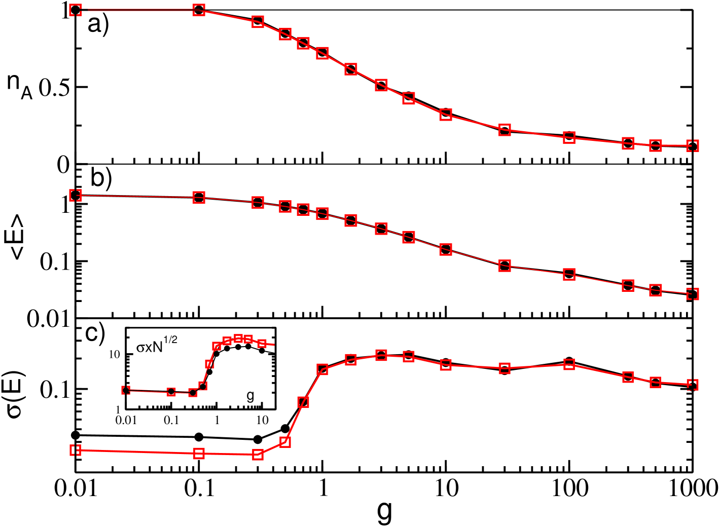
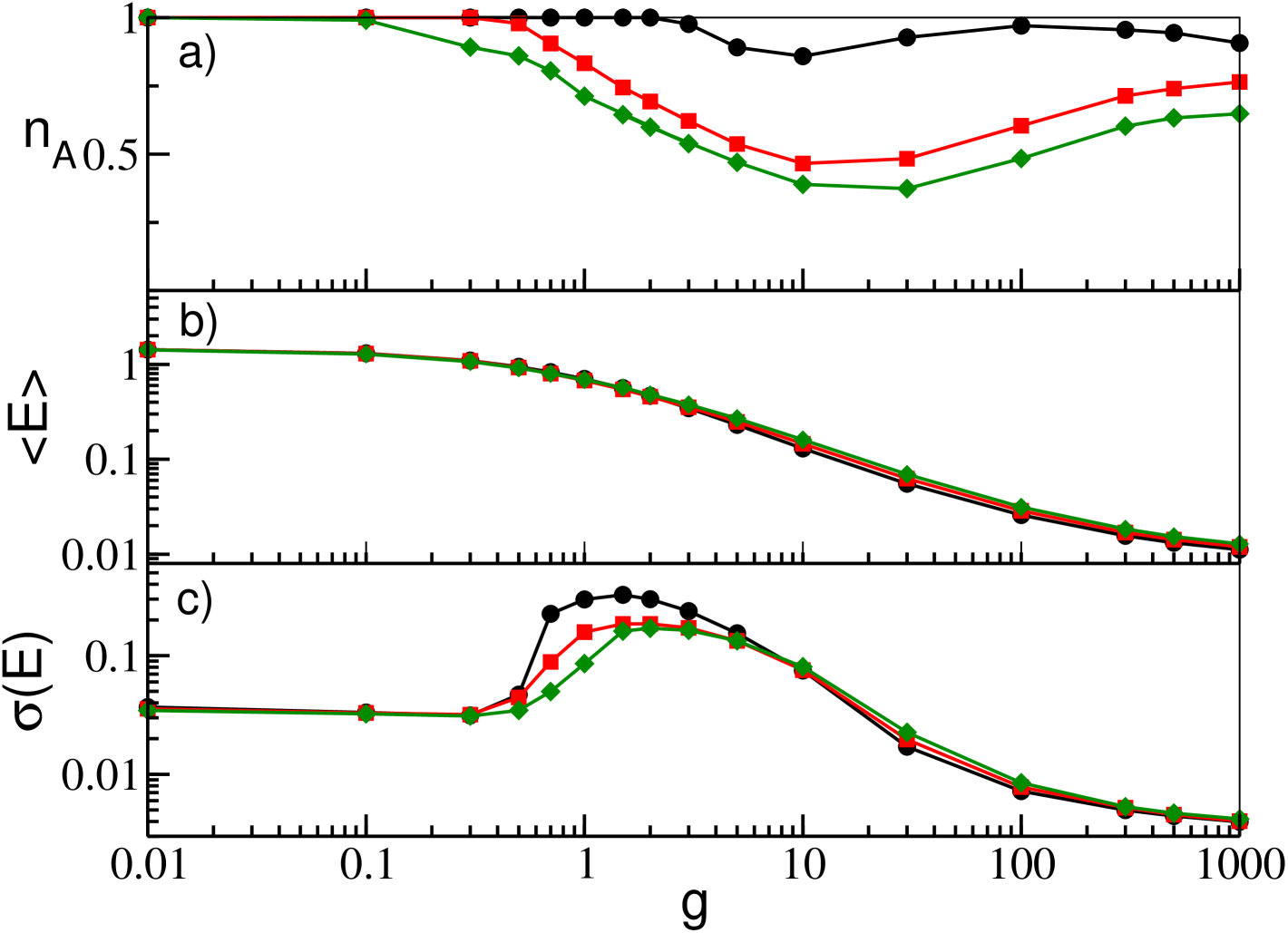
First we will examine how the dynamics of a GCN will change for increasing synaptic coupling strengths , for a chosen time delay and a certain quenched distribution of the neuronal excitability. The results of this analysis are reported in Fig. 1 (a-c) for two different system sizes, namely and . Analogously to what found in absence of delay in Angulo-Garcia et al. (2017), we observe a steady decrease of the value of for increasing and essentially no dependence on the system size. Furthermore, the value of is independent of the value of the considered time period once a transient time is discarded.
For sufficiently small coupling all the neurons are active (i.e., ), and the field , which is a proxy of the firing activity of the network, presents an almost constant value with few or none fluctuations. This indicates an asynchronous activity Olmi et al. (2012), as confirmed by the raster plot shown in Fig. 1 (d) for . By increasing the coupling, reduces below one, because now the neuronal population splits in two groups : one displaying a high activity, the winners, which are able to mute the other group of neurons, the losers, which are usually characterized by lower values of the excitability . Further increases in the inhibition produces a steady decrease of the percentage of active neurons due to the increased inhibitory action of the winners that induces an enlargement of the family of the losers and an associated decrease in the network activity measured by as shown in Fig. 1 (b). This is clearly an effect, which can be attributed to the WTA mechanism.
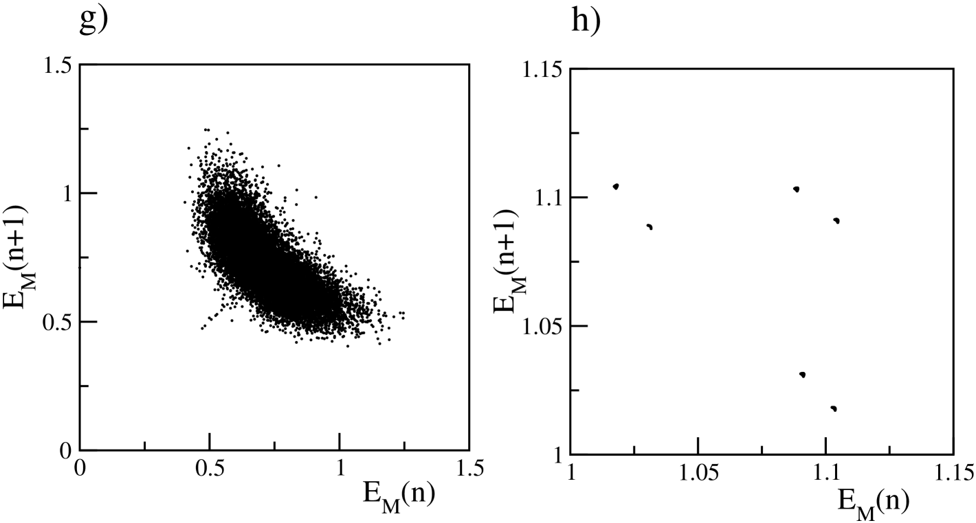
In Ernst et al. (1995) it has been shown that perfectly synchronized clusters of neurons emerge in homogeneous fully coupled inhibitory networks due to the transmission delay. The presence of disorder (either in the excitability distribution or in the connections) leads to a smearing of the clusters associated to a non perfect synchronization Politi and Luccioli (2010); Luccioli and Politi (2010); Zillmer et al. (2009) as we observe in the present case. As shown in Fig. 1 (e) and (f), for sufficiently large , the emergence of the partially synchronized clusters produce collective oscillations at the macroscopic level. In particular, we observe a transition from an asynchronous state to collective oscillations, as demonstrated in Fig. 1 (c) by reporting as a function of for different system sizes. At tends to vanish as , a typical signature of asynchronous dynamics, for larger values of the coupling strength (namely ), displays a finite value independent of the system size signaling the presence of collective oscillations. The nature of these oscillations has been previously extensively analysed in Luccioli and Politi (2010). In such study the authors have shown that at intermediate coupling strengths the collective dynamics is irregular, despite the linear stability of the system, due to stable chaos mechanisms Politi and Torcini (2010). This is evident from Fig. 1 (e), where the first return map for the maxima of the field is reported for . In the present analysis we examine much larger coupling strength than in Politi and Torcini (2010), namely . At these large synaptic strenghts we observe that the complexity of the collectve dynamics reduces due to the fact that the number of active neurons drastically declines, as shwon in Fig. 1 (a). The few active neurons have a quite limited spread in their excitabilities (namely not ) thus promoting their reciprocal synchronization. This is also evident from the sharp peaks in the mean field evolution (see Fig.1 (f)) and from the periodic behaviour of the first return map of , shown in Fig.1 (h).
III.1 Role of the heterogeneity and the delay
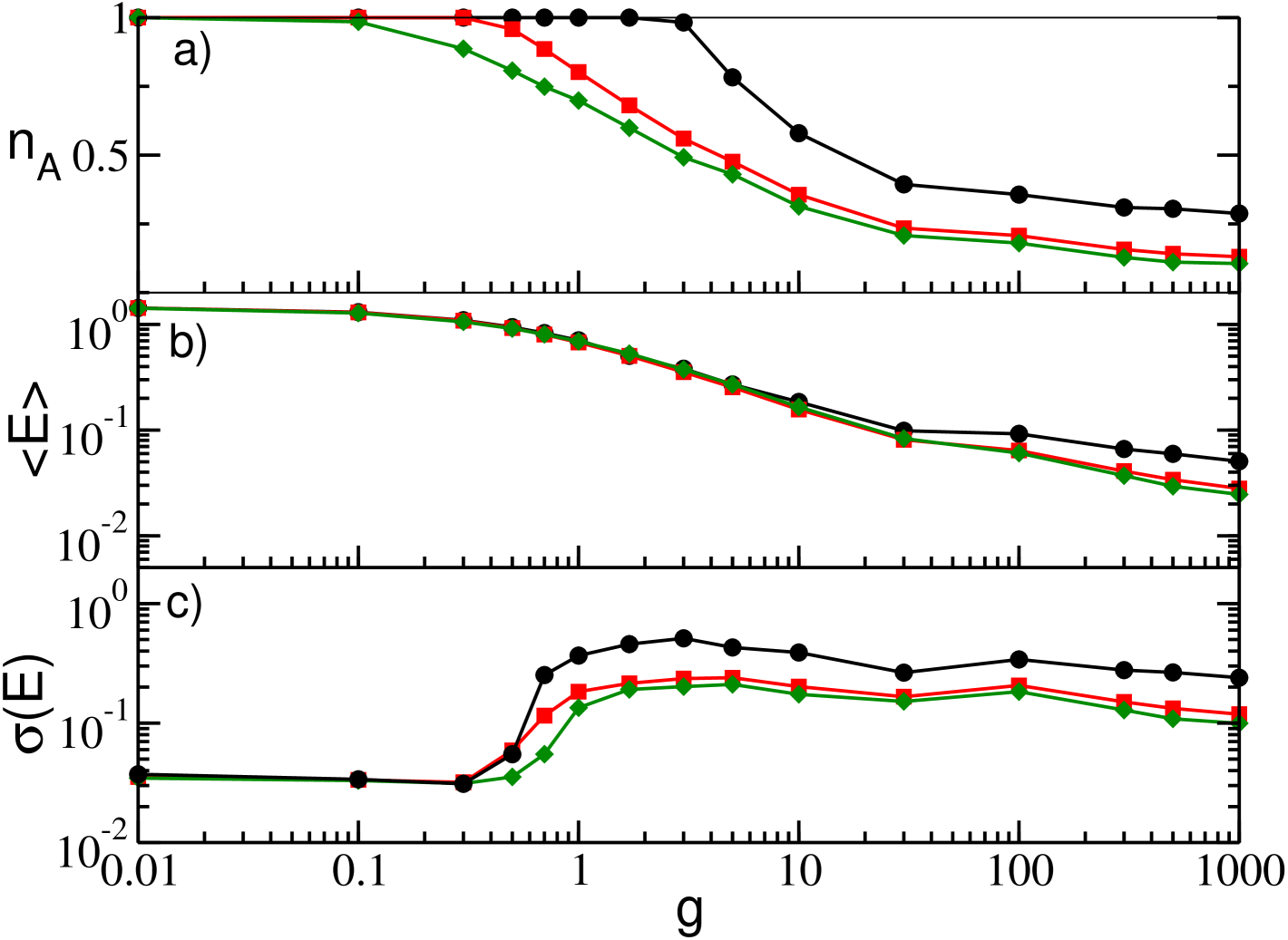
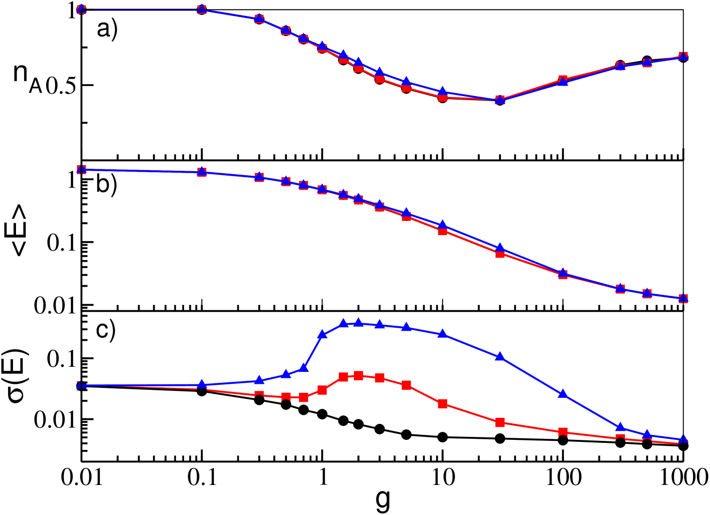
To better understand the influence on the dynamics of the parameters entering in the model, we considered different distributions of the excitabilities and different time delays . Let us first consider heterogeneity distributions with different widths , but with the same average value , for a fixed value of the delay (namely, ). As shown in Fig. 2 (a) and as already demonstrated in case of absence of delay Angulo-Garcia et al. (2017) for (corresponding to in the present case) any arbitrary small amount of inhibition is sufficient to induce neuronal deactivation. However, for increasing values of (for decreasing widths ) the onset of neuronal deactivation occurs at increasingly larger -values, since larger amount of inhibition are required to silence the neurons with smallest excitability. This also explains why the values of the curves decrease for increasing , as shown in Fig. 2 (a).
The average mean field does not present significant modifications with as seen in Fig. 2 (b). This is due to the fact that, from a mean field perspective, the system is subject to the same average excitability and hence one does not expect large deviations in the average firing rates. There are only small deviations at very large where the network with wider dispersion in the excitabilities display slightly smaller firing rates, just because the number of active neurons is drastically decreased. This effect is much more evident in Fig. 2 (c), where we can observe that the value of significatively affects both the onset and the amplitude of the collective oscillations as measured by . This because the decrease of brings to a reduction in the number of partially synchronized neurons and in turn of the amplitude of the fluctuations of the field.
Let us now consider the influence of the time delay, for a fixed heterogeneity distribution. From Fig. 3 (a), it appears that approaches an asymptotic plateau for very large coupling, whose value steadily decreases for increasing . Indeed, for very small delays the survivors reduce to few units, e.g. see the example reported in Fig. 3 (a) for . This dependence of on the delay at large couplings is confirmed also by the corresponding values of the field shown in Fig. 3 (b). Overall, longer synaptic delays counteract the effect of the heterogeneity and therefore the neural deactivation, as a matter of fact for the fraction of active neuron is still for g=1000 (data not shown).
Furthermore, the delay has a crucial role in the emergence of collective oscillations that can be observed already for extremely small delay, e.g for the parameters considered in Fig. 3 (c). Indeed, no collective oscillations have been observed in heterogeneous GCN in absence of delay at any coupling stregth Angulo-Garcia et al. (2017). By increasing the delay we observe larger and larger oscillations in the field , as shown by the curves reported in Fig. 3 (c).
These behaviours can be explained by the fact that collective oscillations are due to the presence of clusters of neurons at a microscopic level. As shown in Ernst et al. (1995, 1998) for homogeneous systems and confirmed in Politi and Luccioli (2010) for heterogenous networks the average number of clusters increases proportionally to the inverse of the delay. Therefore for small delay we expect to observe an asynchronous state, characterized by , while for increasing delay decreases and thus the neurons are more and more synchronized, thus promoting larger collective fluctuations. The increase in the overall synchronization leads to a reduced effective variability in the neuron dynamics, thus preventing neuronal deactivation. Indeed, disorder promotes deactivation as demonstrated in Angulo-Garcia et al. (2017) in absence of delay and as shown in Fig. 2 (a), where is reported for various values.
IV Sparse Network
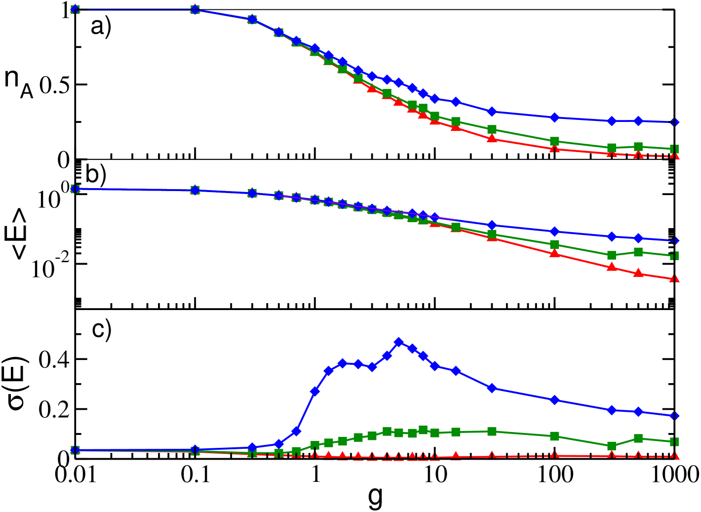
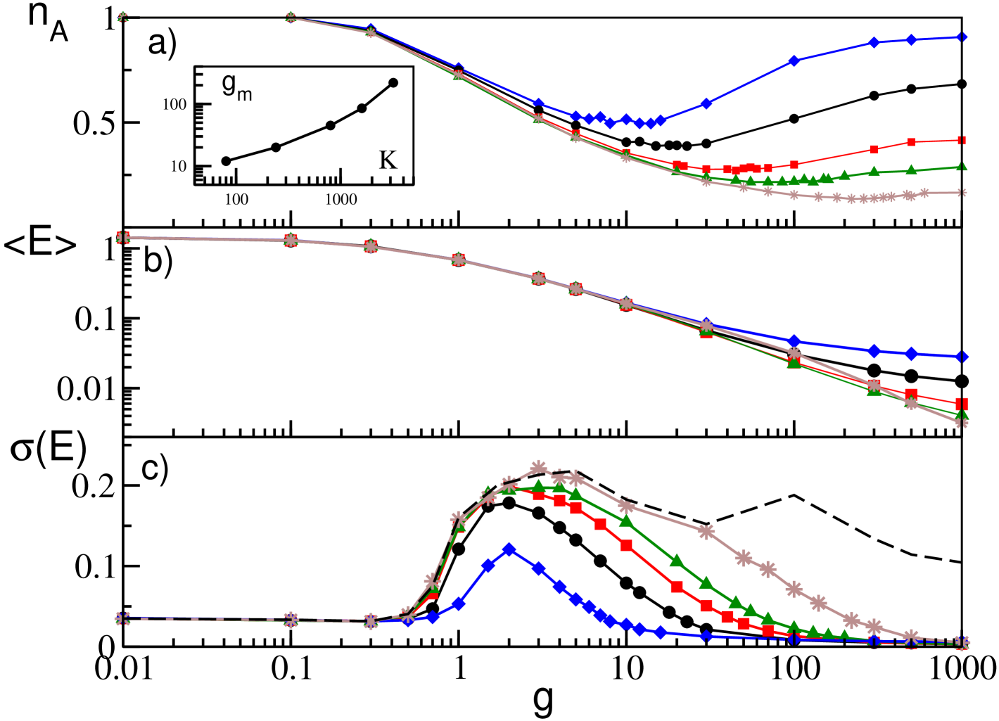
We will now consider the diluted case, i.e. each neuron has now exactly random pre-synaptic neighbours. In this case we observe that has a non-monotonic behaviour with , as shown in Fig. 4 (a) for different values of the in-degree for a fixed system size, namely . In particular, we observe that for small coupling shows a decrease analogous to the one reported for the GCN, hower for for synaptic coupling larger than a critical value the percentage of active neurons increases with . This behaviour indicates that large inhibtory coupling can lead to a reactivation of previously inactive neurons in sparse networks, as prevously reported in inhibtory networks in absence of delay for conductance based Ponzi and Wickens (2013) and LIF neuronal models Angulo-Garcia et al. (2015, 2017). The value of grows faster than a power-law with the in-degree , as shown in the inset of Fig. 4 (a). In particular, we expect that for , i.e. by recovering the fully coupled case, and converges towards the curve reported in Fig. 1 (a).
Analogously to GCNs the average mean field is steadily decreasing with indicating that the neuronal dynamics slow down for increasing inhibition and that for sufficiently large all the neurons can eventually be reactivated but with a definitely low firing rate. The dependence of on , shown in Fig. 4 (b), reveals that for essentially all curves coincide, while at larger synaptic coupling the smaller is the larger is the value of the field, this behaviour is clearly dictated by that of . More neurons are reactivated, higher is the filtered firing rate measured by .
The mean field fluctuations have now a striking different behaviour with respect to the GCN, because now displays a maximum at some intermediate value, while for small and large coupling tends to vanish, as shown in Fig. 4 (c). This suggests that collective oscillations are present only at intermediate coupling, while out of this range the dynamics is asynchronous. This is confirmed by the raster plots and the fields reported in Fig. 4 (d-f) for different synaptic couplings. At small coupling (namely, ) a clear asynchronous state, characterized by an almost constant , is observable , while in an intermediate range of synaptic couplings clear collective oscillations are present, as testified by the raster plot and the field shown in Fig. 4 (e) for . Furthermore, for sufficiently large coupling the asynchronous dynamics is characterized by a sporadic bursting activity with an intra-burst period corresponding to to of the considered neuron, as shown for in Fig. 4 (f).
From Fig. 4 (c) it is also evident that the onset and the amplitude of the collective dynamics strongly depend on the dilution measured in terms of the in-degree , and that for the globally coupled behavior is recovered. In particular, smaller is smaller is the amplitude of the collective oscillations and narrower is the synaptic coupling interval where they are observable. These two effects are due to the fact that the disorder in the connectivity distribution increases as . Therefore, on one side the clusters of partially synchronized neurons, which are responsible for the collectivve oscillations, are more smeared at smaller thus inducing smaller amplitudes of the oscillations. On the other side, the disorder prevent the emergence of collective oscillations, thus the region of existence is reduced at lower . As a matter of fact, for 4000 we start to observe collective oscillations only when . The existence of a critical connectivity for the emergence of collective dynamics is a general feature of sparse networks Luccioli et al. (2012); di Volo and Torcini (2018).

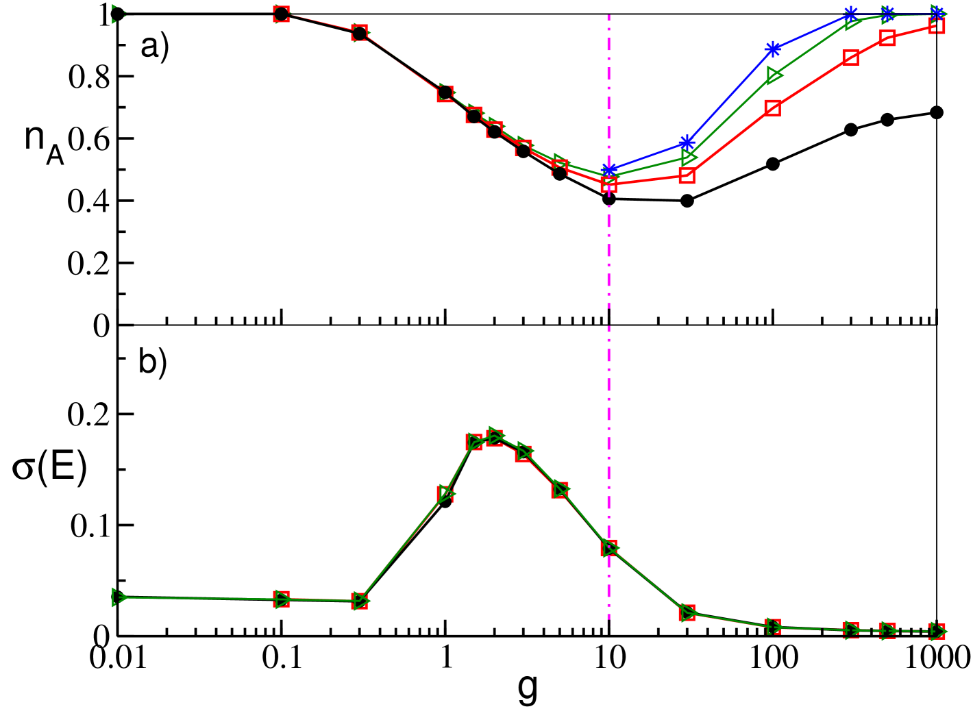
In order to understand if the value of the time interval over which we measure and has an influence on the observed effects, let us examine the dependence of these two quantities on for a fixed size and in-degree . The results of this analysis reported in Fig. 5 show that for the percentage of active neurons is almost insensible to the considered time window, similarly to what observed for the GCN. On the other hand, for the value grows with and for sufficiently long times and for sufficiently large eventually all the neurons can be reactivated. However, as shown in Fig. 5 (a) the growth noticeably slow down for increasing and we can safely affirm that for the further evolution of occurs on unrealistic long time scales. For what concerns finite time effects are essentially not present, as shown in Fig. 5 (b).
IV.1 The role of current fluctuations
Previous analysis of inhibitory networks in absence of delay Ponzi and Wickens (2013); Angulo-Garcia et al. (2015, 2017) have clearly shown that the position of the minimum of marks the transition from a regime dominated by the activity of the supra-threshold neurons (mean driven) to a regime where the most part of the neurons are below threshold and the firing is mainly due to current fluctuations (fluctuation driven) Renart et al. (2007).
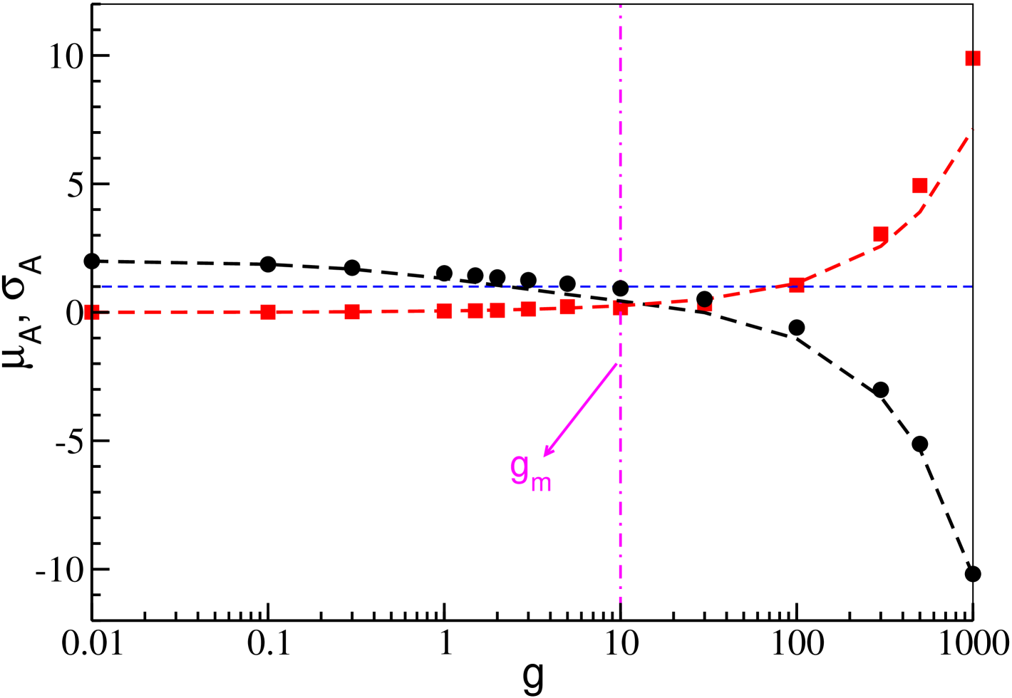
In order to verify if also in the present case the origin of the neuronal reactivation is related to such a transition, let us analyze the system at a mean-field level, in this framework the activty of a neuron is completely determined by the average input current and by its fluctuations. Let us limit our analysis to the active neurons, since these are the only ones contributing to the network dynamcs, in particular the average effective input to the active neurons can be estimated as follows
| (4) |
where () is the average excitability (firing rate) of the active neurons. The current fluctuations can be estimated by following Tuckwell (2005); Brunel and Hakim (1999), despite the dynamics is fully deterministic, thanks to the disorder induced by the sparsness in the connections each neuron can be seen as subject to uncorrelated Poissonian trains of inhibitory spikes of constant amplitude and characterized by an average firing rate . Therefore the current fluctuations can be estimated as follows:
| (5) |
As it can be appreciated from Fig. 6, the theoretical estimations (4) and (5) (dashed curves) are in very good agreement with the numerical data for and (filled symbols) over the whole considered range of the synaptic inhibition (corresponding to five orders of magnitude). In the same figure, one observes a steady decrease of with , which can be understood from its expression (4), since is a quantity monotonically decreasing with the synaptic strenght despite the neural reactivation present in SNs. This can be inferred from the behaviour of the mean field , which is strictly connected to , reported in Fig. 4 (b). On the other hand, the fluctuations of the input currents increase with , thus indicating that in (5) the growth of prevails over the decrease of .
The key result explaining the mechanism behind neural reactivation is reported in Fig. 6: it is clear that becomes smaller than the firing threshold exactly at , in concomitance with a dramatic growth of the current fluctuations. Therefore for , since all the neurons are on average below threshold, the neural firing is mostly due to current fluctuations and not to the intrinsic excitability of each neuron. Therefore we expect that for large coupling strength, on one side the average firing of the neurons will become slower, as indeed shown in Fig. 4 (b), while on the other side the fraction of firing neurons will increase, thanks to the increase of with . Therefore we can confirm that the occurrence of the minimum in signals a transition from a mean driven to a fluctuation driven dynamics, analogously to what found in Angulo-Garcia et al. (2017) in absence of delay.
However, in the present case current fluctuations have also a destructive role on the collective dynamics induced by the delay. As it can be inferred from Fig. 5 (b) (see also Fig. 11 in the last section), the coherent motion disappears as soon as due to the random fluctuations in the input currents which completely desynchronize the neural activity.
IV.2 Characterization of the microscopic dynamics
The analysis of the microscopic dynamics can clarify the different observed regimes. In particular, we will consider the dynamics of the neurons in a network with and in three typical regimes: namely, in presence of collective motion (), in proximity of the minimum of () and for very large inhibition (). In particular, for each synaptic coupling we study the distribution of the ISIs, , for three representative neurons characterized by high (H), intermediate (I) and low (L) average firing rates.
The results of this analysis are reported in Fig. 7, where we considered (a,b), (c) and (d). In particular, corresponds to the maximum in the amplitude of the collective oscillations measured by (see Fig. 5). For this synaptic coupling the distrbutions are quite peculiar, being characterized by several peaks separated by a constant time lag . The number of peaks and the value of increase going from the fastest to the slowest neuron: namely, the time lag varies from (F) to (I) and (L).
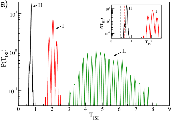
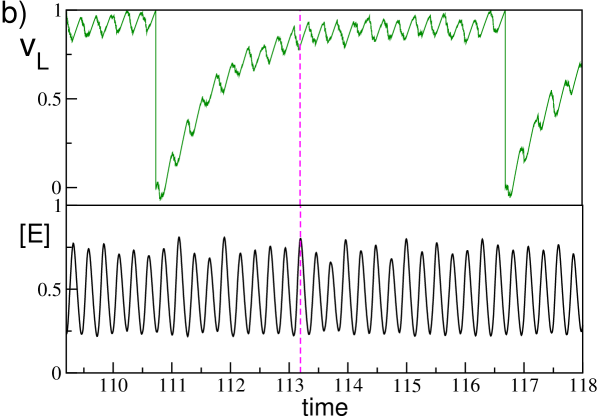
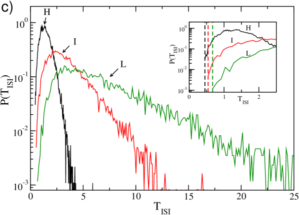
This structure can be traced back to the coherent inhibitory action of clusters of partially synchronized neurons, coarse grained by the collective field , on the targeted neuron. This effect is shown in Fig. 7 (b), where on the same time interval are reported the membrane potential of the neuron with low firing rate and . The average field displays irregular oscillations due to the clustered activity of the neurons, furthermore it is clear that the occurrence of every local maximum in is in perfect correspondence with a local minimum of . Therefore, a spike can be emitted only in correspondence of a local minimum of the field, thus the of neuron (L) should be multiples of the oscillation period of , which is . The locking with the collective field is progressively less effective for the neurons with higher firing rates (namely, (I) and (H)) and this reduces the multi-peak structure and the value of . Moreover, in this regime dominated by collective inhibitory oscillations the minimal for each neuron is definitely larger than the corresponding . Obviously, the more active the neuron is, the closer to is the minimal (see the inset in Fig. 7 (a)).
For larger values of , the collective oscillations vanish and accordingly the multi-peak structure in disappears, while the statistics of the firing times becomes essentially Poissonian as shown in Fig. 7 (c). Moreover, starting from the coupling strength , where no more collective effects are present the free spiking period appears as the minimal of the distributions (see the inset in Fig. 7 (c)).
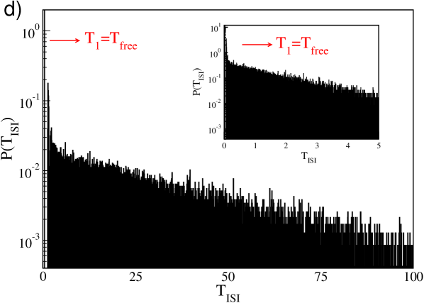
Finally, in the regime of very large , an interesting phenomenon emerges shown in Fig. 7 (d) for : the ISI distribution displays a large peak at and and exponential tail, a typical signature of Poissonian firing. This structure is due to the bursting activity of the neuron (see also Fig. 4 (f)). Indeed, for this large coupling the firing rate of the pre-synaptic neurons is very low, therefore the post-synaptic neurons are usually not inhibited and fire with their free spiking period . However, whenever they receive sporadically inhibitory kicks of large amplitude , the neurons are silent for the long period necessary to the membrane potential to recover positive values. Furthermore, the Poissonian nature of the distribution of the kick arrival times, due to the network sparsness, reflects in the long tail of the .
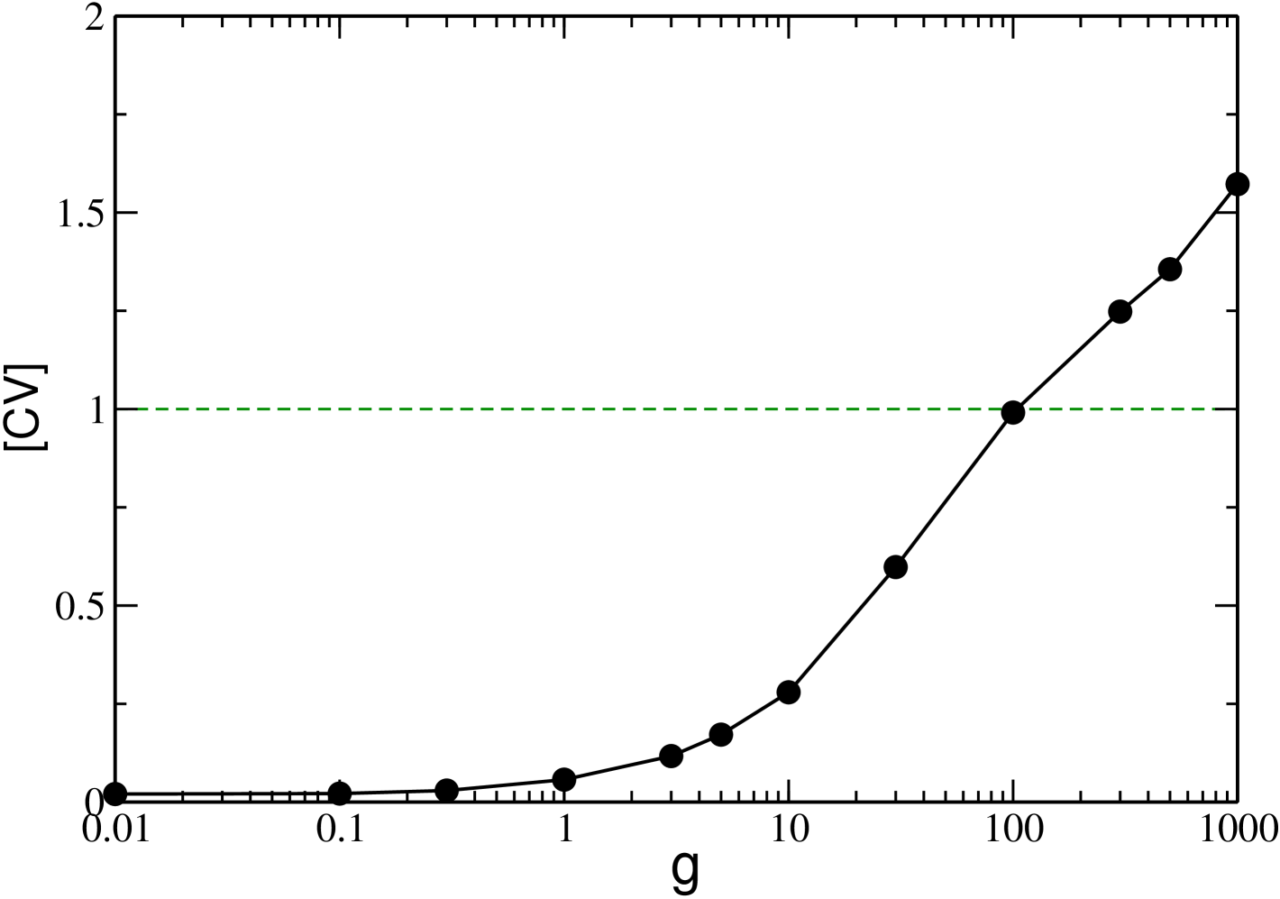
Overall, upon increasing inhibition, on one side we observe that the average frequency of neurons steadily decreases, on the other side the neurons tend to fire occasionally at the fastest possible frequency, namely . This behaviour is joined to a steadily increasing variability in the microscopic firing of the neurons, as clearly shown in Fig. 8 where we report the ensemble average of the coefficients of variation, . In particular, we observe upon increasing , a transition from a very regular firing characterized by to a dynamics with , which is a signature of multi-modal ISI distributions.
IV.3 Role of the heterogeneity and of the delay
Analogously to what done for the GCNs, we analyzed the influence of different excitability distributions as well as of the time delay on the dynamics of SNs. The results of these analyses are reported in Figs. 9 and 10.
In order to study the effect of the heterogeneity in the neuronal excitabilities, we choose to mantain constant the average =2 and to vary . As discussed in the previous sub-sections, heterogeneity is necessary for the WTA mechanism to kick in. Therefore for small the overall deactivation-reactivation effect is less evident, because the percentage of inactive neurons is much smaller then at larger and the complete reactivation of all neurons is obtained at relatively smaller (see Fig. 9 (a)). Similarly to the GCNs, the average network activity as measured by remains unchanged, because it is mainly dictated by the average synaptic current (see Fig. 9 (b)). Finally, also in this case, the value of affects the onset and the amplitude of the collective motion (see Fig. 9 (c)), due to the same mechanism already discussed for GCNs.
Regarding the delay, it is worth to remind that in the globally coupled system the effects of the synaptic delays were observable for and only at large inhibition, where the WTA mechanism reduces largely the number of active neurons. This effect is not present in SNs due to the reactivation process occurring at sufficiently large (see Fig. 10 (a,b)). However, similarly to the GCNs, the collective activity can emerge only for sufficiently long delays, namely , and the amplitude of the collective oscillations, measured by increases with as shown in Fig. 10 (c).
V Finite size effects
In this Section we report a detailed analysis of the effects of the disorder on finite size networks. In GCNs the only source of disorder is associated to the distribution of the excitabilites, while in SNs, the disorder is due also to the random distribution of the connections. In both cases we consider for each system size 10 different network realizations, which implies different excitability and connectivity distributions.
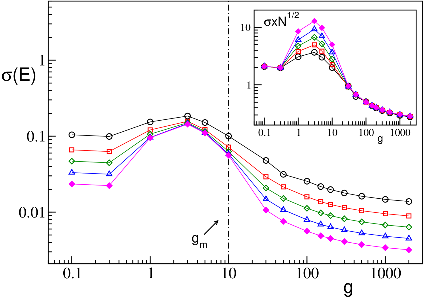
Let us first consider the field and its fluctuations , similarly to what reported for the GCNs (see Fig. 1 (b)) also for the SNs the average value of does not depend on (data not shown). Instead, the mean field fluctuations strongly depend on the size , as shown also for the GCNs in Fig. 1 (c). In particular, for SNs we report as a function of in Fig. 11 for a fixed in-degree for system sizes ranging from to . From the figure (and the inset) it is clear that for and indicating that in the thermodynamic limit the dynamics is asynchronous for small and large couplings. For intermediate values of (namely ) saturates, for sufficiently large , to an asymptotic finite value, thus showing clearly the persistence of the collective behaviour in the thermodynamic limit. From this analysis we can conclude that the collective oscillations are present in an interval of which remains finite in the thermodynamic limit and whose width is determined by the value of (as shown in Fig. 4 (c)) but not by the size . Furthermore, for SNs with sufficiently long delay we have two phase transitions: from asynchronous to collective behaviour (at small coupling) and from collective to asynchronous dynamics (at large ).
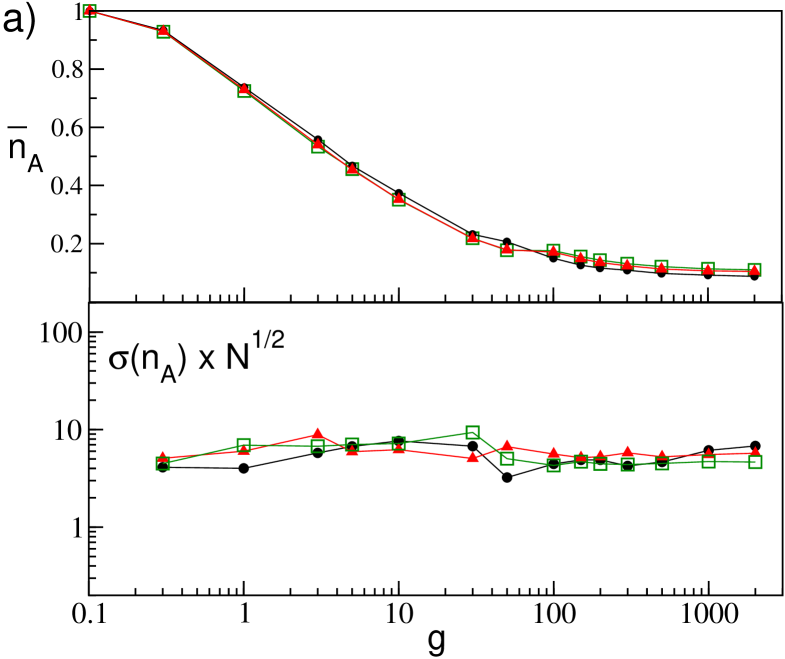
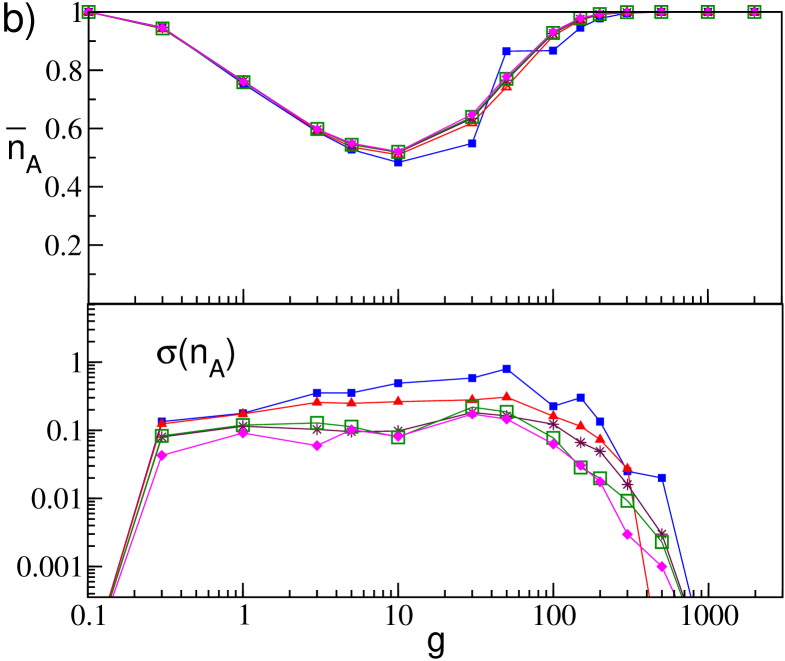
Let us now consider the effect of the realizations of disorder on the percentage of active neurons. In particular, in Fig. 12 we report the average, , and the standard deviation, , of the fraction of active neurons obtained for 10 different network realizations for increasing both for GCNs an SNs. As a general remark we observe that is not particularly sensible to the system size, apart for really small sizes () in the SN case (see the upper panels in Fig. 12 (a) and (b)). The case of small network sizes for SNs will be discussed in the following of this Section.
For what concerns for the GCNs we observe, as expected, a decrease as with the system size, as clearly evident from the lower panel in Fig. 12 (a). Moreover we observe that is essentially constant over the whole range of the coupling strength, apart the case of very small coupling strength, (not shown in the figure), where due to the essentially uncoupled dynamics of the neurons for every . The behavior is quite different for SNs as it is shown in Fig. 12 (b) for networks with . As a general remark we observe that whenever (i.e. for and ) the fluctuations vanish and exhibit finite values in the range of synaptc strenght where . Furthermore, for increasing the values of saturate towards an asymptotic profile. Therefore the fluctuations will persist even in the thermodynamic limit, in agreement with the results reported in Luccioli et al. (2012), and they assume an almost constant value () in the range of existence of collective oscillations (namely, ).
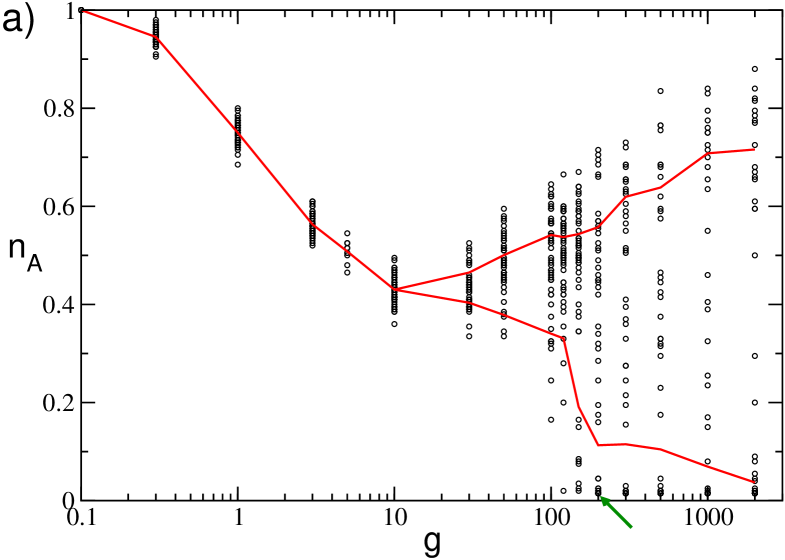
The sparsness of the network can give rise to striking effects for small system size, as it is shown in Fig. 13. In particular, in Fig. 13 (a) we report the values of for 50 different realizations of the network for and . For small coupling strength, namely , we observe that the distribution of values has a single peak centered around the average . While, for larger coupling strength the distribution reveals two distinct peaks: one associated to the typical dynamics of a sparse network at large (i.e. neural reactivation) and one to the typical dynamics of a GCN (i.e. the WTA mechanism). Thus rendering the definition of quite questionable. As a matter of fact, for we estimated two distinct averages for each , one based on the values larger than and one on the smaller values, these are reported as red lines in Fig. 13 (a). We observe this coexistence of two different type of dynamics also by considering different initial conditions for a fixed disorder realization (data not shown).
A peculiar dynamical state can be observed for sufficiently large , denoted by a green arrow in Fig. 13 (a). In this case the corresponding raster plot (shown in Fig. 13 (b)) reveals, after a short transient, the convergence towards a dynamical state where only few neurons survive (namely, three in this case), while the rest of the network becomes silent. The interesting aspect is that these three neurons are completely uncoupled among them and their activity is sufficient to silence all the rest of the neurons. The microscopic analysis reveals that the three neurons have high intrinsic excitability (but not the highest) and that the ensemble of their post-synaptic neurons correspond to the whole network, apart themselves.

The reported effects, i.e. the coexistence of different dynamics as well as the existence of states made of totally uncoupled neurons, disappear increasing the system size. As a matter of fact these effects are already no more observable for .
VI Concluding remarks
In this paper we have clarified how in an inhibitory spiking network the introduction of various ingredients, characteristic of real brain circuits, like delay in the electric signal transmission, heterogeneity of the neurons and random sparseness in the synaptic connections, can influence the neural dynamics.
In particular, we have studied at a macroscopic and microscopic level the dynamics of heterogeneous inhibitory spiking networks with delay for increasing synaptic coupling. In GCNs the heterogeneity is responsible for neuron’s death via the WTA mechanism, while the delay allows for the emergence of COs beyond a critical coupling strength. Furthermore, we have shown that the increase in the delay favours the overall collective dynamics (synchronization) in the system, thus reducing the effective variability in the neuron dynamics. Therefore, longer delays counteract the effect of heterogeneity in the system, which promotes neural deactivation and asynchronous dynamics.
In SNs by increasing the coupling we observe a passage from a mean driven to a fluctuation driven dynamics induced by the sparsness in the connections. We have a transition from a regime where the neurons are on average supra-threshold to a phase where they are on average below-threshold and their firing is induced by large fluctuations in the currents. This transition is signaled by the occurrence of a minimum in the value of the fraction of active neurons as a function of the inhibitory coupling. Therefore we can affirm that we pass from a regime dominated by the WTA mechanism, to an activation regime controlled by fluctuations, where all neurons are finally firing but with firing rates definitely lower then those dictated by their excitabilities Angulo-Garcia et al. (2017). However, the fluctuations desynchronize the neural dynamics: the COs emerging at small coupling, due to the time delay, disappear at large coupling when current fluctuations become predominant in the neural dynamics.
Finite size analysis confirm that in SNs we have two phase transitions that delimit the finite range of couplings where COs are observable. Outside this range the dynamics is asynchronous, however we have two different kinds of asynchronous dynamics at low and high coupling. At low coupling, we observe a situation where the firing variability of each neuron is quite low and essentially the active neurons behave almost independently. At large coupling, the variability of the firing activity is extremely large, characterized by a bursting behaviour at the level of single neurons. Due to the sparsness and the low activity of the fluctuations activated pre-synaptic neurons, each neuron is subject to low rate Poissonian spike trains of PSPs of large amplitude. Therefore the neurons are for long time active and unaffected by the other neurons, however when they receive large inhibitory PSPs they remain silent for long periods.
It has been shown that heterogeneity and noise can increase the information encoded by a population counteracting the correlation present in neuronal activity Shamir and Sompolinsky (2006); Padmanabhan and Urban (2010); Ecker et al. (2011); Mejias and Longtin (2014, 2012). However, it remains to clarify how disorder (neural heterogeneity and randomness in the connections) and delay should combine to enhance information encoding. The results reported in this paper can help in understanding the influence of delay and disorder on the dynamics of neural circuits and therefore on their ability to store and recover information.
Acknowledgements.
The authors acknowledge N. Brunel, V. Hakim, S. Olmi, for enlightening discussions. AT has received partial support by the Excellence Initiative I-Site Paris Seine (No ANR-16-IDEX-008), by the Labex MME-DII (No ANR-11-LBX-0023-01) and by the ANR Project ERMUNDY (No ANR-18-CE37-0014) all funded by the French programme “Investissements d’Avenir”. DA-G has received financial support from Vicerrectoria de Investigaciones - Universidad de Cartagena (Project No. 085-2018) and from CNRS for a research period at LPTM, UMR 8089, Université de Cergy-Pontoise, France. The work has been partly realized at the Max Planck Institute for the Physics of Complex Systems (Dresden, Germany) as part of the activity of the Advanced Study Group 2016/17 “From Microscopic to Collective Dynamics in Neural Circuits”.References
- Ben-Ari (2001) Y. Ben-Ari, Trends in neurosciences 24, 353 (2001).
- Jonas and Buzsaki (2007) P. Jonas and G. Buzsaki, Scholarpedia 2, 3286 (2007).
- Whittington et al. (2000) M. A. Whittington, R. Traub, N. Kopell, B. Ermentrout, and E. Buhl, International journal of psychophysiology 38, 315 (2000).
- Buzsaki (2006) G. Buzsaki, Rhythms of the Brain (Oxford University Press, USA, 2006), 1st ed., ISBN 0195301064.
- Buzsáki and Chrobak (1995) G. Buzsáki and J. J. Chrobak, Current opinion in neurobiology 5, 504 (1995).
- Salinas and Sejnowski (2001) E. Salinas and T. J. Sejnowski, Nature reviews neuroscience 2, 539 (2001).
- van Vreeswijk (1996) C. van Vreeswijk, Phys. Rev. E 54, 5522 (1996).
- Ernst et al. (1995) U. Ernst, K. Pawelzik, and T. Geisel, Physical review letters 74, 1570 (1995).
- Friedrich and Kinzel (2009) J. Friedrich and W. Kinzel, Journal of computational neuroscience 27, 65 (2009).
- Zillmer et al. (2006) R. Zillmer, R. Livi, A. Politi, and A. Torcini, Phys. Rev. E 74, 036203 (2006).
- Brunel and Hakim (1999) N. Brunel and V. Hakim, Neural. Comput. 11, 1621 (1999).
- Brunel (2000) N. Brunel, J. Comput. Neurosci. 8, 183 (2000), ISSN 0929-5313.
- Politi and Luccioli (2010) A. Politi and S. Luccioli, in Network Science: Complexity in Nature and Technology (Springer, London, 2010), p. 217.
- Golomb and Hansel (2000) D. Golomb and D. Hansel, Neural computation 12, 1095 (2000).
- di Volo and Torcini (2018) M. di Volo and A. Torcini, Physical review letters 121, 128301 (2018).
- Coultrip et al. (1992) R. Coultrip, R. Granger, and G. Lynch, Neural networks 5, 47 (1992).
- Fukai and Tanaka (1997) T. Fukai and S. Tanaka, Neural computation 9, 77 (1997).
- Itti and Koch (2001) L. Itti and C. Koch, Nature reviews neuroscience 2, 194 (2001).
- Lee et al. (1999) D. K. Lee, L. Itti, C. Koch, and J. Braun, Nature neuroscience 2, 375 (1999).
- Wang (2002) X.-J. Wang, Neuron 36, 955 (2002).
- Wong and Wang (2006) K.-F. Wong and X.-J. Wang, Journal of Neuroscience 26, 1314 (2006).
- Fries et al. (2007) P. Fries, D. Nikolić, and W. Singer, Trends in neurosciences 30, 309 (2007).
- Angulo-Garcia et al. (2017) D. Angulo-Garcia, S. Luccioli, S. Olmi, and A. Torcini, New Journal of Physics 19, 053011 (2017).
- Ponzi and Wickens (2013) A. Ponzi and J. R. Wickens, PLoS computational biology 9, e1002954 (2013).
- Angulo-Garcia et al. (2015) D. Angulo-Garcia, J. D. Berke, and A. Torcini, PLoS Comput Biol 12, e1004778 (2015).
- Olmi et al. (2012) S. Olmi, A. Politi, and A. Torcini, The Journal of Mathematical Neuroscience 2, 12 (2012).
- Luccioli and Politi (2010) S. Luccioli and A. Politi, Phys. Rev. Lett. 105, 158104+ (2010).
- Zillmer et al. (2009) R. Zillmer, N. Brunel, and D. Hansel, Phys. Rev. E 79, 031909 (2009).
- Politi and Torcini (2010) A. Politi and A. Torcini, in Nonlinear Dynamics and Chaos: Advances and Perspectives (Springer, 2010), pp. 103–129.
- (30) The winners are the neurons with higher values of the excitability. In the case of a uniform distribution defined in the interval the smallest excitability of an active neuron is . Therefore the spread of the excitabilities of the ative neuron is given by .
- Ernst et al. (1998) U. Ernst, K. Pawelzik, and T. Geisel, Phys. Rev. E 57, 2150 (1998).
- Luccioli et al. (2012) S. Luccioli, S. Olmi, A. Politi, and A. Torcini, Phys. Rev. Lett. 109, 138103 (2012).
- Renart et al. (2007) A. Renart, R. Moreno-Bote, X.-J. Wang, and N. Parga, Neural. Comput. 19, 1 (2007).
- Tuckwell (2005) H. C. Tuckwell, Introduction to theoretical neurobiology: Volume 2, nonlinear and stochastic theories, vol. 8 (Cambridge University Press, 2005).
- Shamir and Sompolinsky (2006) M. Shamir and H. Sompolinsky, Neural computation 18, 1951 (2006).
- Padmanabhan and Urban (2010) K. Padmanabhan and N. N. Urban, Nature neuroscience 13, 1276 (2010).
- Ecker et al. (2011) A. S. Ecker, P. Berens, A. S. Tolias, and M. Bethge, Journal of Neuroscience 31, 14272 (2011).
- Mejias and Longtin (2014) J. F. Mejias and A. Longtin, Frontiers in computational neuroscience 8, 107 (2014).
- Mejias and Longtin (2012) J. Mejias and A. Longtin, Physical Review Letters 108, 228102 (2012).