Neural Microfacet Fields for Inverse Rendering
Abstract
We present Neural Microfacet Fields, a method for recovering materials, geometry, and environment illumination from images of a scene. Our method uses a microfacet reflectance model within a volumetric setting by treating each sample along the ray as a (potentially non-opaque) surface. Using surface-based Monte Carlo rendering in a volumetric setting enables our method to perform inverse rendering efficiently by combining decades of research in surface-based light transport with recent advances in volume rendering for view synthesis. Our approach outperforms prior work in inverse rendering, capturing high fidelity geometry and high frequency illumination details; its novel view synthesis results are on par with state-of-the-art methods that do not recover illumination or materials.
![[Uncaptioned image]](https://cdn.awesomepapers.org/papers/7ce36141-d723-4a65-a69a-32e7c9094544/x1.png)
1 Introduction
Simultaneous recovery of the light sources illuminating a scene and the materials and geometry of objects inside it, given a collection of images, is a fundamental problem in computer vision and graphics. This decomposition enables editing and downstream usage of a scene: rendering it from novel viewpoints, and arbitrarily changing the scene’s illumination, geometry, and material properties. This disentanglement is especially useful for creating 3D assets that can be inserted into other environments and realistically rendered under novel lighting conditions.
Recent methods for novel view synthesis based on neural radiance fields [27] have been highly successful at decomposing scenes into their geometry and appearance components, enabling rendering from new, unobserved viewpoints. However, the geometry and appearance recovered are often of limited use in manipulating either materials or illumination, since they model each point as a direction-dependent emitter rather than as reflecting the incident illumination. To tackle the task of further decomposing appearance into illumination and materials, we return to a physical model of light-material interaction, which models a surface as a distribution of microfacets that reflect light rather than emitting it. By explicitly modeling this interaction during optimization, our method can recover both material properties and the scene’s illumination.
Our method uses a Monte Carlo rendering approach with a hybrid surface-volume representation, where the scene is parameterized as a 3D field of microfacets: the scene’s geometry is represented as a volume density, but its materials are parameterized using a spatially varying Bidirectional Reflectance Distribution Function (BRDF). The volumetric representation of geometry has been shown to be effective for optimization [27, 44], and treating each point in space as a microfaceted surface allows us to use ideas stemming from decades of prior work on material parameterization and efficient surface-based rendering. Despite its volumetric parameterization, we verify experimentally that our model shrinks into a surface around opaque objects, with all contributions to the color of a ray coming from the vicinity of its intersection with the object.
To summarize, our method (1) combines aspects of volume-based and surface-based rendering for effective optimization, enabling reconstructing high-fidelity scene geometry, materials, and lighting from a set of calibrated images; (2) uses an optimizable microfacet material model rendered using Monte Carlo integration with multi-bounce raytracing, allowing for realistic interreflections on nonconvex objects; and (3) is efficient: it optimizes a scene from scratch in 3 hours on a single NVIDIA GTX 3090.
2 Related work
Our work lies in the rich field of inverse rendering, in which the goal is to reconstruct the geometry, material properties, and illumination that gave rise to a set of observed images. This task is a severely underconstrained inverse problem, with challenges ranging from lack of differentiability [22] to the computational cost-variance tradeoff of the forward rendering process [17].
Recent progress in inverse rendering, and in particular in view synthesis, has been driven by modeling scenes as radiance fields [27, 3, 4], which can produce photorealistic models of a scene based on calibrated images.
Inverse rendering.
Inverse rendering techniques can be categorized based on the combination of unknowns recovered and assumptions made. Common assumptions include far field illumination, isotropic BRDFs, and no interreflections or self-occlusions. Early work by Ramamoorthi and Hanrahan [33] handled unknown lighting, texture, and BRDF by using spherical harmonic representations of both BRDF and lighting, which allowed recovering materials and low frequency lighting components. More recent methods used differentiable rendering of known geometry, first through differentiable rasterization [24, 23, 9] and later through differentiable ray tracing [22, 2, 31]. Later methods built on differentiable ray tracing, making use of Signed Distance Fields (SDFs) to also reconstruct geometry [46, 29, 17].
Following the success of NeRF [27], volumetric rendering has emerged as a useful tool for inverse rendering. Some methods based on volume rendering assume known lighting and only recover geometry and materials [37, 5, 1], while others solve for both lighting and materials, but assume known geometry [25, 49] or geometry without self-occlusions [7, 6]. Some methods simultaneously recover illumination, geometry, and materials, but assume that illumination comes from a single point light source [16, 45]. However, to the best of our knowledge none of these existing volumetric inverse rendering methods are able to capture high frequency lighting (and appearance of specular objects) from just the input images themselves.
An additional challenge is in handling multi-bounce illumination, or interreflections, in which light from a source bounces off multiple objects before reaching the camera. In this case, computational tradeoffs are unavoidable due to the exponential growth of rays with the number of such bounces. Park et al. [31] model interreflections assuming known geometry, but do not model materials, which is equivalent to treating all objects as perfect mirrors. Other methods use neural networks to cache visibility fields [37, 49] or radiance transfer fields [25, 16]. Our method handles interreflections by casting additional rays through the scene, using efficient Monte Carlo sampling.
Volumetric view synthesis.
We base our representation of geometry on recent advances in volumetric view synthesis, following NeRF [27]. Specifically, we retain the idea of using differentiable volumetric rendering to model geometry, using a voxel-based representation of the underlying density field [14, 28, 8].
Of particular relevance to our work are prior methods such as [41, 15] that are specifically designed for high-fidelity appearance of glossy objects. In general, most radiance field models fail at rendering high-frequency appearance caused by reflections from shiny materials under natural illumination, instead rendering blurry appearance [47]. To enable our method to handle these highly specular materials, and to improve the normal vectors estimated by our method, which are key to the rendered appearance, we utilize regularizers from Ref-NeRF [41].
3 Preliminaries
Our method combines aspects of volumetric and surface-based rendering; we begin with a brief introduction to each before describing our method in Section 4.
3.1 Volume Rendering
The core idea in emission-absorption volume rendering is that light accumulates along rays, with “particles” along the ray both emitting and absorbing light. The color measured by a camera pixel corresponding to a ray with origin and direction is:
| (1) | ||||
| (2) |
where is a camera ray, is the density at point in the volume, denotes transmittance along the ray, and is the outgoing radiance. This formula is often approximated numerically using quadrature, following [26]:
| (3) | ||||
| (4) | ||||
| (5) |
In this volume rendering paradigm, multiple 3D points can contribute to the color of a ray, with nearer and denser points contributing most.
3.2 Surface Rendering
In surface rendering, and assuming fully-opaque surfaces, the color of a ray is determined solely by the light reflected by the first surface it encounters. Consider that the ray from camera position in direction intersects its first surface at a 3D position . The ray color is then:
| (6) |
where is the direction of incident light, is the surface normal at , is the BRDF describing the material of the surface at , is the incident radiance, and is a truncated cosine lobe (i.e. its negative values are clipped to zero) facing outward from the surface. Note that this equation is recursive: inside the integral may be the outgoing radiance coming from a different scene point. The integral in Equation 6 is also typically approximated by discrete (and often random) sampling, and is the subject of a rich body of work [11, 40].
4 Method
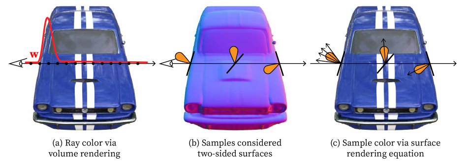
We present Neural Microfacet Fields to tackle the problem of inverse rendering by combining volume and surface rendering, as shown in Figure 2. Our method takes as input a collection of images ( in our experiments) with known cameras, and outputs the volumetric density and normals, materials (BRDFs), and far-field illumination (environment map) of the scene. We assume that all light sources are infinitely far away from the scene, though light may interact locally with multiple bounces through the scene.
In this section, we describe our representation of a scene and the rendering pipeline we use to map this representation into pixel values. Section 4.1 introduces the main idea of our method, to build intuition before diving into the details. Section 4.2 describes our representation of the scene geometry, including density and normal vectors. Section 4.3 describes our representation of materials and how they reflect light via the BRDF. Section 4.4 introduces our parameterization of illumination, which is based on a far-field environment map equipped with an efficient integrator for faster evaluations of the rendering integral. Finally, Section 4.5 describes the way we combine these different components to render pixel values in the scene.
4.1 Main Idea
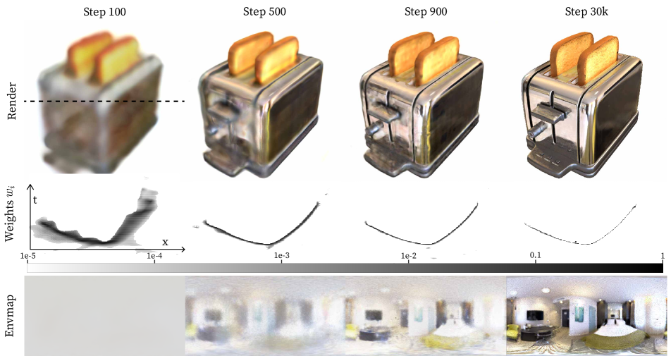
The key to our method is a novel combination of the volume rendering and surface rendering paradigms: we model a density field as in volume rendering, and we model outgoing radiance at every point in space using surface-based light transport (approximated using Monte Carlo ray sampling). Volume rendering with a density field lends itself well to optimization: initializing geometry as a semi-transparent cloud creates useful gradients (see Figure 3), and allows for changes in geometry and topology. Using surface-based rendering allows modeling the interaction of light and materials, and enables recovering these materials.
We combine these paradigms by modeling a microfacet field, in which each point in space is endowed with a volume density and a local micro-surface. Light accumulates along rays according to the volume rendering integral of Equation 1, but the outgoing light of each 3D point is determined by surface rendering as in Equation 6, using rays sampled according to its local micro-surface. This combination of volume-based and surface-based representation and rendering, shown in Figure 2, enables us to optimize through a severely underconstrained inverse problem, recovering geometry, materials, and illumination simultaneously.
4.2 Geometry Parameterization
We represent geometry using a low-rank tensor data structure based on TensoRF [8], with small modifications described in Appendix C. Our model stores both density and a spatially-varying feature that is decoded into the material’s BRDF at every point in space. We initialize our model at low resolution and gradually upsample it during optimization (see Appendix C for details).
Similar to prior work [37, 41], we use the negative normalized gradient of the density field as a field of “volumetric normals.” However, like [20], we found that numerically computing spatial gradients of the density field using finite differences rather than using analytic gradients leads to normal vectors that we can use directly, without using features predicted by a separate MLP. Additionally, these numerical gradients can be efficiently computed using 2D and 1D convolution using TensorRF’s low-rank density decomposition (see Appendix C). These accurate normals are then used for rendering the appearance at a volumetric microfacet, as will be discussed in Sections 4.3 and 4.5.
Our volumetric normals are regularized using the orientation loss introduced by Ref-NeRF [41]:
| (7) |
where is the view direction facing towards the camera, and is the normal vector at the th point along the ray. The orientation loss penalizes normals that face away from the camera yet contribute to the color of the ray (as quantified by weights ).
Because our volumetric normals are derived from the density field, this regularizer has a direct effect on the reconstructed geometry: it decreases the weight of backwards-facing normals by decreasing their density or increasing the density between them and the cameras, thereby promoting hard surfaces and improving reconstruction. Note that unlike Ref-NeRF, we do not use “predicted normals” for surface rendering, as our Gaussian-smoothed derivative filter achieves similar effect.
4.3 Material Representation
We write our spatially varying BRDF model as a combination of diffuse and specular components:
| (8) |
where is the RGB albedo, is the half vector, is the Fresnel term, is the specular component of the BRDF for outgoing view direction and incident light direction . The spatial dependence of these terms on the point is omitted for brevity. We use the Schlick approximation [35] for the Fresnel term:
| (9) |
where is the spatially varying reflectance at the normal incidence at the point , and we base our specular BRDF on the Cook-Torrance BRDF [38], using:
| (10) |
where is a Trowbridge-Reitz distribution [39] (popularized by the GGX BRDF model [42]), is the Smith shadow masking function for the Trowbridge-Reitz distribution, and is a shallow multilayer perceptron (MLP) with a sigmoid nonlinearity at its output. The distribution models the roughness of the material, and it is used for importance sampling, as described in Section 4.5). The MLP captures other material properties not included in its explicit components.
The parameters for each of the diffuse and specular BRDF components are stored as features in the TensoRF representation (alongside density ), allowing them to vary in space. We compute the roughness , albedo and reflectance at the normal incidence by applying a single linear layer with sigmoid activation to the spatially-localized features . Details about the architecture of the MLP and its input encoding can be found in Appendix B.
We can approximately evaluate the rendering equation integral in Equation 6 more efficiently by assuming all microfacets at a point have the same irradiance :
| (11) | ||||
| (12) |
The irradiance , defined as:
| (13) |
can then be easily evaluated using an irradiance environment map approximated by low-degree spherical harmonics, as done by Ramamoorthi and Hanrahan [32]. At every optimization step, we obtain the current irradiance environment map by integrating the environment map with spherical harmonic functions up to degree , and combining the result with the coefficients of a clamped cosine lobe pointing in direction to obtain the irradiance [32]. Equation 4.3 can then be importance sampled according to and integrated using Monte Carlo sampling of incoming light.
We sample half vectors from the distribution of visible normals [18], which is defined as:
| (14) |
However, to perform Monte Carlo integration of the rendering equation, we need to convert from half vector space to the space of incoming light, which requires multiplying by the determinant of the Jacobian of the reflection equation , which is [42]. Multiplying by the term from Equation 6 as well as the Jacobian and Equation 14 results in the following Monte Carlo estimate:
| (15) | ||||
4.4 Illumination
We model far field illumination using an environment map, represented using an equirectangular image with dimensions , with and . We map the optimizable parameters in our environment map parameterization into high dynamic range RGB values by applying an elementwise exponential function.
We use the term primary to denote a ray originating at the camera, and secondary to denote a ray bounced from a surface to evaluate its reflected light (whether that light arrives directly from the environment map, or from another scene point).
To minimize sampling noise, instead of using a single environment map element per secondary ray, we use the mean value over an axis-aligned rectangle in spherical coordinates, with the solid angle covered by the rectangle adjusted to match the sampling distribution at that point. Concretely, to query the environment map at a given incident light direction, we first compute its corresponding spherical coordinates , where and are the polar and azimuthal angles respectively. We then compute the mean value of the environment map over a (spherical) rectangle centered at , whose size we constrain to have aspect ratio . To choose the solid angle of the rectangle, , we modify the method from [10], which is based on Nyquist’s sampling theorem (see Appendix A). We compute these mean values efficiently using integral images, also known as summed-area tables [13].
4.5 Rendering
In this section, we describe how the model components representing geometry (Section 4.2), materials (Section 4.3), and illumination (Section 4.4) are combined to render the color of a pixel. For each primary ray, we choose a set of sample points following the rejection-sampling strategy of [21, 28] to prioritize points near object surfaces. We query our geometry representation [8] for the density at each point, and use Equation 4 to estimate the contribution weight of each point to the final ray color.
To compute the color for each of these points, we compute the irradiance from the environment map and apply Equation 4.3 to obtain , as described in Section 4.3.
For each primary ray sample with weight , we allocate secondary rays, where is an upper bound on the total number of secondary rays for each primary ray (since ). The secondary rays are sampled according to the Trowbridge-Reitz distribution using the normal vector and roughness value at the current sample.
When computing the incoming light , we save memory by randomly selecting a fixed number of secondary rays to interreflect through the scene while others index straight into the environment map. We importance sample these secondary rays according to the largest channel of the weighted RGB multiplier . In practice, we find that adding a small amount of random noise to the weighted RGB multiplier before choosing the largest values improves performance by slightly increasing the variation of the selected rays.
The remaining secondary rays with lower contribution are rendered more cheaply by evaluating the environment map directly rather than considering further interactions with the scene, as described in Section 4.4.
This combined sample color value is then weighted by , and the resulting colors are summed along the primary ray samples to produce pixel values. Finally, the resulting pixel values are tonemapped to sRGB color and clipped to .
Dynamic batching.
We apply the dynamic batch size strategy from NeRFAcc [21] to the TensoRF [8] sampler, which controls the number of samples per batch using the number of primary rays per batch. Since the number of secondary rays scales with the number of primary rays, we bound the maximal number of primary rays to avoid casting too many secondary rays. We use the same method to control , the number of secondary bounces that retrace through the scene. During test time, we shuffle the image to match the training distribution, then unshuffle the image to get the result.
5 Experiments
We evaluate our method using two synthetic datasets: the Blender dataset from NeRF [27], and the Shiny Blender dataset from Ref-NeRF [41]. Both datasets contain objects rendered against a white background; the Shiny Blender dataset focuses on shiny materials with high-frequency reflections whereas the Blender dataset contains a mixture of specular, glossy, and Lambertian materials.
We evaluate standard metrics PSNR, SSIM [43], and LPIPS [48] on the novel view synthesis task for each dataset. To quantify the quality of our reconstructed geometry, we also evaluate the Mean Angular Error (MAE∘) of the normal vectors. MAE∘ is evaluated over the same test set of novel views; for each view we take the dot product between the ground truth and predicted normals, multiply the of this angle by the ground truth opacity of the pixel, and take the mean over all pixels. This gives us an error of if the predicted normals are missing (i.e. if the pixel is mistakenly predicted as transparent). We summarize these quantitative metrics in Table 1, with per-scene results in Appendix D.
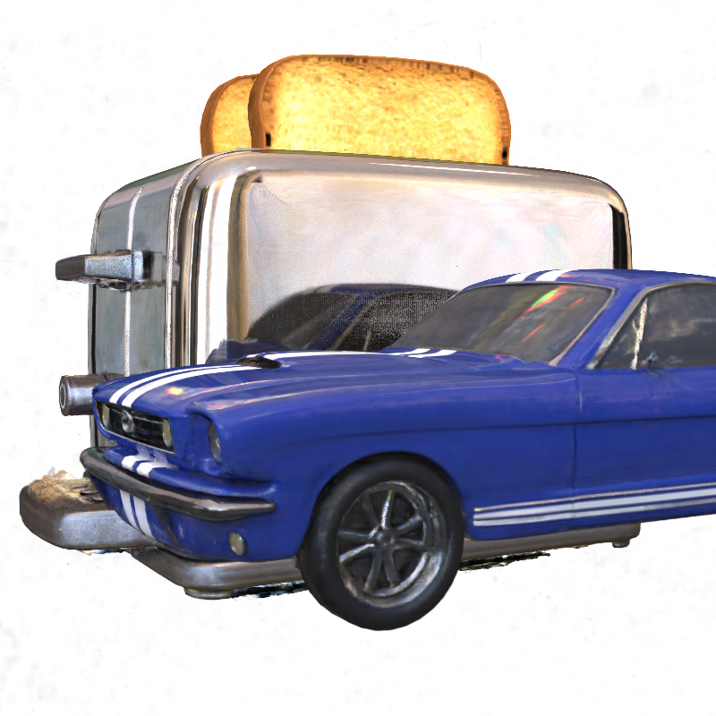
We provide qualitative comparisons of our reconstructed environment maps with prior inverse rendering approaches in Figures 5 and 6, and additional results in Appendix D. We also demonstrate two applications of our scene decomposition in Figure 4. For Figure 4 (a), we render the geometry and spatially varying BRDF recovered from the materials scene with the environment map optimized from the helmet scene, showing convincing new reflections while retaining the original object shape and material properties. For Figure 4 (b), we take this a step further by training the toaster and car scenes with the same neural material decoder, which enabled us to compose the two scenes under the environment map recovered from the toaster scene.
To quantitatively measure the quality of our method’s disentanglement, we evaluate it similarly to NeRFactor [49]. Since our method is specifically designed to handle more specular objects, we modify the Shiny Blender dataset from Ref-NeRF [41] by rendering the images in HDR under both the original lighting and an unseen lighting condition. We then optimize each method on each of the scenes with original lighting, then render the estimated geometry and materials using the unseen lighting condition. For computing quality metrics, we find the (ambiguous) per-channel scaling factor by minimizing the mean squared error. The scaled image is then evaluated against the ground truth relit image using PSNR, SSIM, and LPIPS.
The results are presented in Table 2, showing that our method is able to relight shiny objects with significantly increased accuracy when compared to state of the art inverse rendering methods such as NVDiffRec and NVDiffRecMC.
|
|
|
| Materials BRDF | |
|
|
|
| Helmet Lighting |
|
|
| Combined Rendering (a) |
Combined Rendering (b)
Table 1 also shows quantitative ablation studies on our model. If we do not use integral images for the far field illumination (“no integral image”), the sparse gradient on the environment map prevents the model from learning to use it to explain reflections. Using the derivative of the linear interpolation of the density instead of smoothed numerical derivatives (“analytical grad”), results in more holes in the geometry, limiting performance. If we do not utilize multiple ray bounces for interreflections (“single bounce”), all metrics are slightly worse, with most of the errors arising in regions with strong interreflections. Finally, replacing the neural network with the identity function (“no neural”), results in slightly worse performance, especially in regions with strong interreflections.
|
Novel View |
||||
|---|---|---|---|---|
|
Normals |
||||
|
Environment |
||||
| Ground Truth | Ours | NVDiffRec | NVDiffRecMC |
|
Novel View |
|
|
|
|
|---|---|---|---|---|
|
Normals |
|
|
|
|
|
Environment |
||||
| Ground Truth | Ours | NVDiffRec | NVDiffRecMC |
| Blender | Shiny Blender | |||||||
| PSNR | SSIM | LPIPS | PSNR | SSIM | LPIPS | |||
| PhySG1 | 18.54 | .847 | .182 | 29.17 | 26.21 | .921 | .121 | 8.46 |
| NVDiffRec1 | 28.79 | .939 | .068 | 11.788 | 29.90 | .945 | .114 | 31.885 |
| NVDiffRecMC1 | 25.81 | .904 | .111 | 9.003 | 28.20 | .902 | .175 | 28.682 |
| Ref-NeRF2 | \cellcolor[HTML]FFB3B333.99 | \cellcolor[HTML]FFB3B3.966 | \cellcolor[HTML]FFB3B3.038 | 23.22 | \cellcolor[HTML]FFB3B335.96 | \cellcolor[HTML]FFB3B3.967 | \cellcolor[HTML]FFD9B3.059 | 18.38 |
| Ours, no integral image | 28.47 | .920 | .069 | 27.988 | 27.33 | .869 | .170 | 34.118 |
| Ours, analytical derivative | 28.94 | .926 | .064 | 13.976 | 29.22 | .900 | .140 | 24.295 |
| Ours, single bounce | \cellcolor[HTML]FFFFB430.68 | \cellcolor[HTML]FFD9B3.944 | \cellcolor[HTML]FFD9B3.045 | \cellcolor[HTML]FFD9B36.216 | \cellcolor[HTML]FFFFB434.39 | \cellcolor[HTML]FFFFB4.962 | \cellcolor[HTML]FFB3B3.053 | \cellcolor[HTML]FFD9B317.647 |
| Ours, no neural | 29.40 | .933 | .057 | \cellcolor[HTML]FFFFB47.325 | 33.00 | .955 | \cellcolor[HTML]FFFFB4.063 | \cellcolor[HTML]FFFFB419.190 |
| Ours | \cellcolor[HTML]FFD9B330.71 | \cellcolor[HTML]FFFFB4.940 | \cellcolor[HTML]FFFFB4.053 | \cellcolor[HTML]FFB3B36.061 | \cellcolor[HTML]FFD9B334.56 | \cellcolor[HTML]FFD9B3.963 | \cellcolor[HTML]FFB3B3.053 | \cellcolor[HTML]FFB3B317.497 |
1 requires object masks during training. 2 view synthesis method, not inverse rendering. Red is best, followed by orange, then yellow.
| PSNR | toaster | coffee | helmet | ball | teapot | car | mean |
|---|---|---|---|---|---|---|---|
| NVDiffRec1 | \cellcolor[HTML]FFFFB412.56 | 20.30 | \cellcolor[HTML]FFFFB417.73 | 13.21 | \cellcolor[HTML]FFFFB433.00 | 19.84 | 19.44 |
| NVDiffRecMC1 | \cellcolor[HTML]FFD9B314.55 | \cellcolor[HTML]FFD9B323.39 | \cellcolor[HTML]FFD9B320.44 | \cellcolor[HTML]FFFFB413.23 | 32.51 | \cellcolor[HTML]FFFFB420.09 | \cellcolor[HTML]FFFFB420.70 |
| Ours | \cellcolor[HTML]FFB3B320.05 | \cellcolor[HTML]FFFFB424.21 | \cellcolor[HTML]FFB3B325.69 | \cellcolor[HTML]FFB3B323.50 | \cellcolor[HTML]FFD9B334.37 | \cellcolor[HTML]FFB3B323.19 | \cellcolor[HTML]FFB3B325.17 |
| LPIPS | toaster | coffee | helmet | ball | teapot | car | mean |
| NVDiffRec1 | .378 | .208 | .229 | .467 | .027 | .113 | .237 |
| NVDiffRecMC1 | \cellcolor[HTML]FFFFB4.290 | \cellcolor[HTML]FFFFB4.177 | \cellcolor[HTML]FFFFB4.217 | \cellcolor[HTML]FFFFB4.423 | \cellcolor[HTML]FFFFB4.024 | \cellcolor[HTML]FFFFB4.105 | \cellcolor[HTML]FFFFB4.206 |
| Ours | \cellcolor[HTML]FFB3B3.170 | \cellcolor[HTML]FFD9B3.142 | \cellcolor[HTML]FFB3B3.129 | \cellcolor[HTML]FFB3B3.191 | \cellcolor[HTML]FFB3B3.017 | \cellcolor[HTML]FFB3B3.063 | \cellcolor[HTML]FFB3B3.119 |
| SSIM | toaster | coffee | helmet | ball | teapot | car | mean |
| NVDiffRec1 | .624 | .870 | .824 | .626 | .985 | .853 | .797 |
| NVDiffRecMC1 | \cellcolor[HTML]FFD9B3.741 | \cellcolor[HTML]FFFFB4.913 | \cellcolor[HTML]FFFFB4.861 | \cellcolor[HTML]FFFFB4.761 | \cellcolor[HTML]FFFFB4.986 | \cellcolor[HTML]FFFFB4.869 | \cellcolor[HTML]FFFFB4.855 |
| Ours | \cellcolor[HTML]FFB3B3.864 | \cellcolor[HTML]FFB3B3.910 | \cellcolor[HTML]FFB3B3.918 | \cellcolor[HTML]FFB3B3.897 | \cellcolor[HTML]FFD9B3.987 | \cellcolor[HTML]FFB3B3.917 | \cellcolor[HTML]FFB3B3.916 |
1 requires object masks during training. Red is best, followed by orange, then yellow.
6 Discussion and Limitations
We introduced a novel and successful approach for the task of inverse rendering, using calibrated images alone to decompose a scene into its geometry, far-field illumination, and material properties. Our approach uses a combination of volumetric and surface-based rendering, in which we endow each point in space with both a density and a local microsurface, so that it can both occlude and reflect light from its environment. We verified experimentally that our method, which enjoys both the optimization landscape of volume rendering, as well as the richness and efficiency of surface-based Monte Carlo rendering, provides superior results relative to prior work.
However, our method is not without limitations. First, although it can handle non-convex geometry, it assumes far field illumination and thus performs poorly when this assumption is not satisfied. This issue is most clear in the coffee scene in the Shiny Blender dataset, which has near-field light sources. It also does not handle interreflections very well, since the number of secondary bounces is limited, and due to our acceleration scheme of often directly querying the environment map, as explained in Section 4.5. Our model also does not handle refractive media, which is most clear in the drums and ship scenes in the Blender dataset. Our diffuse lighting model also assumes far field illumination, and thus fails to fully isolate shadows from the albedo, most obvious in the lego scene in the Blender dataset. These scenes are visualized in Appendix D. Another limitation of our model’s BRDF parameterization is that it struggles to represent anisotropic materials. Finally, our method exhibits some speckle noise in its renderings, particularly near bright spots, which may be alleviated by using a denoiser as was used in [17]. We believe these limitations would make for interesting future work, as well as applying our method to other field representations and larger scenes captured in the wild.
7 Acknowledgements
We would like to thank Tzu-Mao Li for his advice, especially regarding the BRDF formulation, as well as his La Jolla renderer, which we used as a reference. AM is supported by ALERTCalifornia, developing technology to stay ahead of disasters, and the National Science Foundation under award #CNS-1338192, MRI: Development of Advanced Visualization Instrumentation for the Collaborative Exploration of Big Data, and Kinsella Expedition Fund. This material is partially based upon work supported by the National Science Foundation under Award No. 2303178 to SFK.
References
- [1] Meghna Asthana, William Smith, and Patrik Huber. Neural apparent brdf fields for multiview photometric stereo. In Proceedings of the 19th ACM SIGGRAPH European Conference on Visual Media Production, pages 1–10, 2022.
- [2] Dejan Azinović, Tzu-Mao Li, Anton Kaplanyan, and Matthias Nießner. Inverse path tracing for joint material and lighting estimation. In Proc. Computer Vision and Pattern Recognition (CVPR), IEEE, 2019.
- [3] Jonathan T. Barron, Ben Mildenhall, Matthew Tancik, Peter Hedman, Ricardo Martin-Brualla, and Pratul P. Srinivasan. Mip-nerf: A multiscale representation for anti-aliasing neural radiance fields. In 2021 IEEE/CVF International Conference on Computer Vision, ICCV 2021, Montreal, QC, Canada, October 10-17, 2021, pages 5835–5844. IEEE, 2021.
- [4] Jonathan T. Barron, Ben Mildenhall, Dor Verbin, Pratul P. Srinivasan, and Peter Hedman. Mip-nerf 360: Unbounded anti-aliased neural radiance fields. In IEEE/CVF Conference on Computer Vision and Pattern Recognition, CVPR 2022, New Orleans, LA, USA, June 18-24, 2022, pages 5460–5469. IEEE, 2022.
- [5] Sai Bi, Zexiang Xu, Pratul Srinivasan, Ben Mildenhall, Kalyan Sunkavalli, Miloš Hašan, Yannick Hold-Geoffroy, David Kriegman, and Ravi Ramamoorthi. Neural reflectance fields for appearance acquisition. arXiv preprint arXiv:2008.03824, 2020.
- [6] Mark Boss, Raphael Braun, Varun Jampani, Jonathan T Barron, Ce Liu, and Hendrik Lensch. Nerd: Neural reflectance decomposition from image collections. In Proceedings of the IEEE/CVF International Conference on Computer Vision, pages 12684–12694, 2021.
- [7] Mark Boss, Varun Jampani, Raphael Braun, Ce Liu, Jonathan Barron, and Hendrik Lensch. Neural-pil: Neural pre-integrated lighting for reflectance decomposition. Advances in Neural Information Processing Systems, 34:10691–10704, 2021.
- [8] Anpei Chen, Zexiang Xu, Andreas Geiger, Jingyi Yu, and Hao Su. Tensorf: Tensorial radiance fields. In European Conference on Computer Vision, pages 333–350. Springer, 2022.
- [9] Wenzheng Chen, Huan Ling, Jun Gao, Edward Smith, Jaakko Lehtinen, Alec Jacobson, and Sanja Fidler. Learning to predict 3d objects with an interpolation-based differentiable renderer. Advances in neural information processing systems, 32, 2019.
- [10] Mark Colbert and Jaroslav Krivanek. Gpu-based importance sampling. GPU Gems, 3:459–476, 2007.
- [11] Robert L Cook and Kenneth E. Torrance. A reflectance model for computer graphics. ACM Transactions on Graphics (ToG), 1(1):7–24, 1982.
- [12] Roy Cranley and Thomas NL Patterson. Randomization of number theoretic methods for multiple integration. SIAM Journal on Numerical Analysis, 13(6):904–914, 1976.
- [13] Franklin C Crow. Summed-area tables for texture mapping. In Proceedings of the 11th annual conference on Computer graphics and interactive techniques, pages 207–212, 1984.
- [14] Sara Fridovich-Keil, Alex Yu, Matthew Tancik, Qinhong Chen, Benjamin Recht, and Angjoo Kanazawa. Plenoxels: Radiance fields without neural networks. In IEEE/CVF Conference on Computer Vision and Pattern Recognition, CVPR 2022, New Orleans, LA, USA, June 18-24, 2022, pages 5491–5500. IEEE, 2022.
- [15] Wenhang Ge, Tao Hu, Haoyu Zhao, Shu Liu, and Ying-Cong Chen. Ref-NeuS: Ambiguity-reduced neural implicit surface learning for multi-view reconstruction with reflection, 2023.
- [16] Michelle Guo, Alireza Fathi, Jiajun Wu, and Thomas Funkhouser. Object-centric neural scene rendering. arXiv preprint arXiv:2012.08503, 2020.
- [17] Jon Hasselgren, Nikolai Hofmann, and Jacob Munkberg. Shape, Light, and Material Decomposition from Images using Monte Carlo Rendering and Denoising. arXiv:2206.03380, 2022.
- [18] Eric Heitz. Sampling the ggx distribution of visible normals. Journal of Computer Graphics Techniques (JCGT), 7(4):1–13, 2018.
- [19] Diederik P Kingma and Jimmy Ba. Adam: A method for stochastic optimization. arXiv preprint arXiv:1412.6980, 2014.
- [20] Zhengfei Kuang, Kyle Olszewski, Menglei Chai, Zeng Huang, Panos Achlioptas, and Sergey Tulyakov. NeROIC: Neural rendering of objects from online image collections. ACM Transactions on Graphics (TOG), 41(4):1–12, 2022.
- [21] Ruilong Li, Matthew Tancik, and Angjoo Kanazawa. Nerfacc: A general nerf acceleration toolbox. arXiv preprint arXiv:2210.04847, 2022.
- [22] Tzu-Mao Li, Miika Aittala, Frédo Durand, and Jaakko Lehtinen. Differentiable monte carlo ray tracing through edge sampling. ACM Trans. Graph., 37(6), dec 2018.
- [23] Shichen Liu, Tianye Li, Weikai Chen, and Hao Li. Soft rasterizer: A differentiable renderer for image-based 3d reasoning. In Proceedings of the IEEE/CVF International Conference on Computer Vision (ICCV), October 2019.
- [24] Matthew M Loper and Michael J Black. Opendr: An approximate differentiable renderer. In Computer Vision–ECCV 2014: 13th European Conference, Zurich, Switzerland, September 6-12, 2014, Proceedings, Part VII 13, pages 154–169. Springer, 2014.
- [25] Linjie Lyu, Ayush Tewari, Thomas Leimkühler, Marc Habermann, and Christian Theobalt. Neural radiance transfer fields for relightable novel-view synthesis with global illumination. arXiv preprint arXiv:2207.13607, 2022.
- [26] N. Max. Optical models for direct volume rendering. IEEE Transactions on Visualization and Computer Graphics, 1(2):99–108, 1995.
- [27] Ben Mildenhall, Pratul P Srinivasan, Matthew Tancik, Jonathan T Barron, Ravi Ramamoorthi, and Ren Ng. Nerf: Representing scenes as neural radiance fields for view synthesis. Communications of the ACM, 65(1):99–106, 2021.
- [28] Thomas Müller, Alex Evans, Christoph Schied, and Alexander Keller. Instant neural graphics primitives with a multiresolution hash encoding. ACM Trans. Graph., 41(4):102:1–102:15, July 2022.
- [29] Jacob Munkberg, Jon Hasselgren, Tianchang Shen, Jun Gao, Wenzheng Chen, Alex Evans, Thomas Mueller, and Sanja Fidler. Extracting Triangular 3D Models, Materials, and Lighting From Images. arXiv:2111.12503, 2021.
- [30] Art B Owen. Randomly permuted (t, m, s)-nets and (t, s)-sequences. In Monte Carlo and Quasi-Monte Carlo Methods in Scientific Computing: Proceedings of a conference at the University of Nevada, Las Vegas, Nevada, USA, June 23–25, 1994, pages 299–317. Springer, 1995.
- [31] Jeong Joon Park, Aleksander Holynski, and Steven M Seitz. Seeing the world in a bag of chips. In Proceedings of the IEEE/CVF Conference on Computer Vision and Pattern Recognition, pages 1417–1427, 2020.
- [32] Ravi Ramamoorthi and Pat Hanrahan. An efficient representation for irradiance environment maps. In Proceedings of the 28th annual conference on Computer graphics and interactive techniques, pages 497–500, 2001.
- [33] Ravi Ramamoorthi and Pat Hanrahan. A signal-processing framework for inverse rendering. In Proceedings of the 28th annual conference on Computer graphics and interactive techniques, pages 117–128, 2001.
- [34] Szymon M Rusinkiewicz. A new change of variables for efficient brdf representation. In Eurographics Workshop on Rendering Techniques, pages 11–22. Springer, 1998.
- [35] Christophe Schlick. An inexpensive brdf model for physically-based rendering. In Computer graphics forum, volume 13, pages 233–246. Wiley Online Library, 1994.
- [36] Ilya Meerovich Sobol. On the distribution of points in a cube and the approximate calculation of integrals. Journal of Computational Mathematics and Mathematical Physics, 7(4):784–802, 1967.
- [37] Pratul P Srinivasan, Boyang Deng, Xiuming Zhang, Matthew Tancik, Ben Mildenhall, and Jonathan T Barron. Nerv: Neural reflectance and visibility fields for relighting and view synthesis. In Proceedings of the IEEE/CVF Conference on Computer Vision and Pattern Recognition, pages 7495–7504, 2021.
- [38] Kenneth E Torrance and Ephraim M Sparrow. Theory for off-specular reflection from roughened surfaces. Josa, 57(9):1105–1114, 1967.
- [39] TS Trowbridge and Karl P Reitz. Average irregularity representation of a rough surface for ray reflection. JOSA, 65(5):531–536, 1975.
- [40] Eric Veach. Robust Monte Carlo methods for light transport simulation. Stanford University, 1998.
- [41] Dor Verbin, Peter Hedman, Ben Mildenhall, Todd Zickler, Jonathan T Barron, and Pratul P Srinivasan. Ref-nerf: Structured view-dependent appearance for neural radiance fields. In 2022 IEEE/CVF Conference on Computer Vision and Pattern Recognition (CVPR), pages 5481–5490. IEEE, 2022.
- [42] Bruce Walter, Stephen R Marschner, Hongsong Li, and Kenneth E Torrance. Microfacet models for refraction through rough surfaces. In Proceedings of the 18th Eurographics conference on Rendering Techniques, pages 195–206, 2007.
- [43] Zhou Wang, Alan C Bovik, Hamid R Sheikh, and Eero P Simoncelli. Image quality assessment: from error visibility to structural similarity. IEEE transactions on image processing, 13(4):600–612, 2004.
- [44] Lior Yariv, Jiatao Gu, Yoni Kasten, and Yaron Lipman. Volume rendering of neural implicit surfaces. In Marc’Aurelio Ranzato, Alina Beygelzimer, Yann N. Dauphin, Percy Liang, and Jennifer Wortman Vaughan, editors, Advances in Neural Information Processing Systems 34: Annual Conference on Neural Information Processing Systems 2021, NeurIPS 2021, December 6-14, 2021, virtual, pages 4805–4815, 2021.
- [45] Kai Zhang, Fujun Luan, Zhengqi Li, and Noah Snavely. Iron: Inverse rendering by optimizing neural sdfs and materials from photometric images. In IEEE Conf. Comput. Vis. Pattern Recog., 2022.
- [46] Kai Zhang, Fujun Luan, Qianqian Wang, Kavita Bala, and Noah Snavely. Physg: Inverse rendering with spherical gaussians for physics-based material editing and relighting. In Proceedings of the IEEE/CVF Conference on Computer Vision and Pattern Recognition, pages 5453–5462, 2021.
- [47] Kai Zhang, Gernot Riegler, Noah Snavely, and Vladlen Koltun. Nerf++: Analyzing and improving neural radiance fields. arXiv preprint arXiv:2010.07492, 2020.
- [48] Richard Zhang, Phillip Isola, Alexei A Efros, Eli Shechtman, and Oliver Wang. The unreasonable effectiveness of deep features as a perceptual metric. In Proceedings of the IEEE conference on computer vision and pattern recognition, pages 586–595, 2018.
- [49] Xiuming Zhang, Pratul P Srinivasan, Boyang Deng, Paul Debevec, William T Freeman, and Jonathan T Barron. Nerfactor: Neural factorization of shape and reflectance under an unknown illumination. ACM Transactions on Graphics (TOG), 40(6):1–18, 2021.
Appendix A Rectangle Size Derivation
As mentioned in Section 4.4 of the main paper, a ray that reaches the environment map is assigned a color taken as the average color over an axis-aligned rectangle in spherical coordinates, where the shape of the rectangle depends on the ray’s direction and the material’s roughness at the ray’s origin. We modify the derivation of the area of the rectangle from GPU Gems [10]. Let be the number of samples, be the probability density function of a given sample direction for viewing direction , and let and be the height and width of the environment map (i.e. its polar and azimuthal resolutions). The density of environment map pixels at a given direction must be inversely proportional to the Jacobian’s determinant, , and it must also satisfy:
| (16) |
and therefore:
| (17) |
The number of pixels per sample, which is the area of the rectangle, is then the total solid angle per sample, multiplied by the number of pixels per solid angle:
| (18) |
where is the polar size of the rectangle, and is its azimuthal size, i.e. the rectangle is , in equirectangular coordinates.
As mentioned in Section 4.4 of the main paper, the aspect ratio of the rectangle is set to:
| (19) |
which yields:
| (20) | ||||
| (21) |
Appendix B BSDF Neural Network Parameterization
Once we have sampled the incoming light directions and their respective values , we transform them into the local shading frame to calculate the value of the neural shading network . We parameterize the neural network with 2 hidden layers of width 64 as , where is the position, are the outgoing and incoming light directions, respectively, and is the normal. However, rather than feeding and to the network directly, we follow the schema laid out by Rusinkiewicz [34] and parameterize the input using the halfway vector and difference vector within the local shading frame , which takes the world space to a frame of reference in which the normal vector points upwards:
| (22) | ||||
| (23) | ||||
| (24) | ||||
| (25) |
where is the cross product. Finally, we encode these two directions using spherical harmonics up to degree 4 (as done in Ref-NeRF [41] for encoding view directions), concatenate the feature vector from the field at point , and pass this as input to the network .
Appendix C Optimization and Architecture
To calculate the normal vectors of the density field, we apply a finite difference kernel, convolved with a Gaussian smoothing kernel with , then linearly interpolate between samples to get the resulting gradient in the 3D volume. We supervise our method using photometric loss, along with the orientation loss of Equation 7. Like TensoRF, we use a learning rate of for the rank and tensor components, and a learning rate of for everything else. We use Adam [19] with . Similar to Ref-NeRF [41], we use log-linear learning rate decay with a total decay of and a warmup of steps and a decay multiplier of over total iterations. This gives us the following formula for the learning rate multiplier for some iteration :
| (26) |
We initialize the environment map to a constant value of . Finally, we upsample the resolution of TensoRF from up to cube-root-linearly at steps , and don’t shrink the volume to fit the model.
To further reduce the variance of the estimated value of the rendering equation (see Equation 4.3), we use quasi-random sampling sequences. Specifically, we use a Sobol sequence [36] with Owens scrambling [30], which gives the procedural sequence necessary for assigning an arbitrary number of secondary ray samples to each primary ray sample. We then apply Cranley-Patterson rotation [12] to avoid needing to redraw samples.
Appendix D Additional Results
Tables 2-5 contain full per-scene metrics for our method as well as ablations and baselines. Visual comparisons are also provided in Figures 7-17.
| \rowcolor[HTML]FFFFFF PSNR | \cellcolor[HTML]FFFFFFteapot | \cellcolor[HTML]FFFFFFtoaster | \cellcolor[HTML]FFFFFFcar | \cellcolor[HTML]FFFFFFball | \cellcolor[HTML]FFFFFFcoffee | \cellcolor[HTML]FFFFFFhelmet | \cellcolor[HTML]FFFFFFchair | \cellcolor[HTML]FFFFFFlego | \cellcolor[HTML]FFFFFFmaterials | \cellcolor[HTML]FFFFFFmic | \cellcolor[HTML]FFFFFFhotdog | \cellcolor[HTML]FFFFFFficus | \cellcolor[HTML]FFFFFFdrums | \cellcolor[HTML]FFFFFFship |
|---|---|---|---|---|---|---|---|---|---|---|---|---|---|---|
| \rowcolor[HTML]FFFFFF PhySG1 | 35.83 | 18.59 | 24.40 | 27.24 | 23.71 | 27.51 | 21.87 | 17.10 | 18.02 | 19.16 | 24.49 | 15.25 | 14.35 | 18.06 |
| \rowcolor[HTML]FFFFFF NVDiffRec1 | 40.13 | 24.10 | 27.13 | 30.77 | 30.58 | 26.66 | 32.03 | 29.07 | 25.03 | 30.72 | 33.05 | \cellcolor[HTML]FFD9B331.18 | 24.53 | 24.68 |
| \rowcolor[HTML]FFFFFF NVDiffRecMC1 | 37.91 | 21.93 | 25.84 | 28.89 | 29.06 | 25.57 | 28.13 | 26.46 | 25.64 | 29.03 | 30.56 | 25.32 | 22.78 | 18.59 |
| \rowcolor[HTML]FFB3B3 \cellcolor[HTML]FFFFFFRef-NeRF2 | 47.90 | \cellcolor[HTML]FFFFFF25.70 | 30.82 | 47.46 | 34.21 | \cellcolor[HTML]FFFFB429.68 | 35.83 | 36.25 | 35.41 | 36.76 | 37.72 | 33.91 | 25.79 | 30.28 |
| \rowcolor[HTML]FFFFFF Ours, no integral image | 42.61 | 18.36 | 25.32 | 21.70 | 31.15 | 24.82 | 30.35 | 30.16 | 25.62 | 30.03 | 33.34 | 28.44 | 24.04 | 25.78 |
| \rowcolor[HTML]FFFFFF Ours, analytical derivative | 43.57 | 21.57 | 27.72 | 22.75 | 31.08 | 28.61 | 30.49 | 30.23 | 28.70 | 31.19 | 33.55 | 27.83 | 24.15 | 25.40 |
| \rowcolor[HTML]FFFFB4 \cellcolor[HTML]FFFFFFOurs, single bounce | 45.23 | \cellcolor[HTML]FFD9B326.91 | 30.13 | 38.38 | 31.39 | \cellcolor[HTML]FFD9B334.32 | \cellcolor[HTML]FFD9B332.57 | 32.83 | 30.92 | \cellcolor[HTML]FFD9B332.49 | 35.07 | 29.24 | \cellcolor[HTML]FFD9B324.99 | 27.32 |
| \rowcolor[HTML]FFFFFF Ours, no neural | 45.21 | \cellcolor[HTML]FFFFB425.73 | 29.03 | 37.41 | 30.99 | 29.63 | 30.62 | 31.00 | 29.37 | 31.29 | 33.88 | 28.10 | 24.52 | 26.44 |
| \rowcolor[HTML]FFD9B3 \cellcolor[HTML]FFFFFFOurs | 45.29 | \cellcolor[HTML]FFB3B327.52 | 30.28 | 38.41 | 31.47 | \cellcolor[HTML]FFB3B334.38 | \cellcolor[HTML]FFFFB432.27 | 32.98 | 31.19 | \cellcolor[HTML]FFFFB432.41 | 35.23 | \cellcolor[HTML]FFFFFF29.24 | \cellcolor[HTML]FFFFB424.96 | 27.37 |
1 requires object masks during training. 2 view synthesis method, not inverse rendering. Red is best, followed by orange, then yellow.
| \rowcolor[HTML]FFFFFF SSIM | \cellcolor[HTML]FFFFFFteapot | \cellcolor[HTML]FFFFFFtoaster | \cellcolor[HTML]FFFFFFcar | \cellcolor[HTML]FFFFFFball | \cellcolor[HTML]FFFFFFcoffee | \cellcolor[HTML]FFFFFFhelmet | \cellcolor[HTML]FFFFFFchair | \cellcolor[HTML]FFFFFFlego | \cellcolor[HTML]FFFFFFmaterials | \cellcolor[HTML]FFFFFFmic | \cellcolor[HTML]FFFFFFhotdog | \cellcolor[HTML]FFFFFFficus | \cellcolor[HTML]FFFFFFdrums | \cellcolor[HTML]FFFFFFship |
|---|---|---|---|---|---|---|---|---|---|---|---|---|---|---|
| \rowcolor[HTML]FFFFFF PhySG1 | .990 | .805 | .910 | .947 | .922 | .953 | .890 | .812 | .837 | .904 | .894 | .861 | .823 | .756 |
| \rowcolor[HTML]FFFFFF NVDiffRec1 | .993 | .898 | .938 | .949 | .959 | .931 | \cellcolor[HTML]FFD9B3.969 | .949 | .923 | \cellcolor[HTML]FFFFB4.977 | \cellcolor[HTML]FFD9B3.973 | \cellcolor[HTML]FFD9B3.970 | .916 | \cellcolor[HTML]FFFFB4.833 |
| \rowcolor[HTML]FFFFFF NVDiffRecMC1 | .990 | .842 | .913 | .849 | .942 | .877 | .932 | .909 | .911 | .961 | .945 | .937 | .906 | .732 |
| \rowcolor[HTML]FFB3B3 \cellcolor[HTML]FFFFFFRef-NeRF2 | .998 | .922 | .955 | .995 | .974 | \cellcolor[HTML]FFFFB4.958 | .984 | .981 | .983 | .992 | .984 | .983 | .937 | .880 |
| \rowcolor[HTML]FFFFFF Ours, no integral image | .994 | .734 | .895 | .753 | .959 | .880 | .946 | .946 | .896 | .962 | .954 | .953 | .905 | .794 |
| \rowcolor[HTML]FFFFFF Ours, analytical derivative | \cellcolor[HTML]FFFFB4.995 | .798 | .925 | .790 | .959 | .930 | .948 | .943 | .936 | .972 | .958 | .950 | .910 | .787 |
| \cellcolor[HTML]FFFFFFOurs, single bounce | \cellcolor[HTML]FFD9B3.996 | \cellcolor[HTML]FFFFB4.909 | \cellcolor[HTML]FFD9B3.951 | \cellcolor[HTML]FFD9B3.983 | \cellcolor[HTML]FFD9B3.962 | \cellcolor[HTML]FFB3B3.971 | \cellcolor[HTML]FFFFB4.964 | \cellcolor[HTML]FFD9B3.966 | \cellcolor[HTML]FFFFB4.957 | \cellcolor[HTML]FFD9B3.978 | \cellcolor[HTML]FFFFB4.969 | \cellcolor[HTML]FFFFB4.959 | \cellcolor[HTML]FFD9B3.922 | \cellcolor[HTML]FFD9B3.835 |
| \rowcolor[HTML]FFFFFF Ours, no neural | \cellcolor[HTML]FFD9B3.996 | .903 | \cellcolor[HTML]FFFFB4.945 | \cellcolor[HTML]FFFFB4.980 | .959 | .947 | .949 | .952 | .945 | .972 | .960 | .954 | .916 | .816 |
| \cellcolor[HTML]FFFFFFOurs | \cellcolor[HTML]FFD9B3.996 | \cellcolor[HTML]FFD9B3.917 | \cellcolor[HTML]FFD9B3.951 | \cellcolor[HTML]FFD9B3.983 | \cellcolor[HTML]FFFFB4.960 | \cellcolor[HTML]FFD9B3.969 | \cellcolor[HTML]FFFFFF.956 | \cellcolor[HTML]FFFFB4.963 | \cellcolor[HTML]FFD9B3.959 | \cellcolor[HTML]FFFFFF.977 | \cellcolor[HTML]FFFFFF.964 | \cellcolor[HTML]FFFFFF.952 | \cellcolor[HTML]FFFFB4.917 | \cellcolor[HTML]FFFFFF.828 |
1 requires object masks during training. 2 view synthesis method, not inverse rendering. Red is best, followed by orange, then yellow.
| LPIPS | teapot | toaster | car | ball | coffee | helmet | chair | lego | materials | mic | hotdog | ficus | drums | ship |
| \rowcolor[HTML]FFFFFF PhySG1 | .022 | .194 | .091 | .179 | .150 | .089 | .122 | .208 | .182 | .108 | .163 | .144 | .188 | .343 |
| \rowcolor[HTML]FFFFFF NVDiffRec1 | .022 | .180 | .057 | .194 | .097 | .134 | \cellcolor[HTML]FFD9B3.027 | .037 | .104 | .033 | \cellcolor[HTML]FFFFB4.038 | \cellcolor[HTML]FFD9B3.030 | .070 | .208 |
| \rowcolor[HTML]FFFFFF NVDiffRecMC1 | .029 | .243 | .086 | .346 | .131 | .215 | .080 | .075 | .096 | .057 | .089 | .076 | .096 | .319 |
| \rowcolor[HTML]FFB3B3 \cellcolor[HTML]FFFFFFRef-NeRF2 | .004 | .095 | \cellcolor[HTML]FFFFFF.041 | \cellcolor[HTML]FFFFFF.059 | \cellcolor[HTML]FFFFFF.078 | \cellcolor[HTML]FFFFB4.075 | .017 | \cellcolor[HTML]FFB3B3.018 | .022 | .007 | .022 | .019 | .059 | \cellcolor[HTML]FFD9B3.139 |
| \rowcolor[HTML]FFFFFF Ours, no integral image | .013 | .285 | .077 | .399 | \cellcolor[HTML]FFD9B3.065 | .180 | .055 | .031 | .074 | .042 | .051 | .039 | .077 | .180 |
| \rowcolor[HTML]FFFFFF Ours, analytical derivative | .011 | .235 | .053 | .353 | .071 | .118 | .052 | .031 | .048 | .028 | .047 | .043 | .075 | .190 |
| \cellcolor[HTML]FFFFFFOurs, single bounce | \cellcolor[HTML]FFD9B3.008 | \cellcolor[HTML]FFFFB4.114 | \cellcolor[HTML]FFB3B3.033 | \cellcolor[HTML]FFD9B3.047 | \cellcolor[HTML]FFB3B3.063 | \cellcolor[HTML]FFB3B3.050 | \cellcolor[HTML]FFFFB4.032 | \cellcolor[HTML]FFB3B3.018 | \cellcolor[HTML]FFD9B3.026 | \cellcolor[HTML]FFD9B3.020 | \cellcolor[HTML]FFD9B3.034 | \cellcolor[HTML]FFFFB4.033 | \cellcolor[HTML]FFD9B3.065 | \cellcolor[HTML]FFB3B3.135 |
| \rowcolor[HTML]FFFFFF Ours, no neural | \cellcolor[HTML]FFD9B3.008 | .115 | \cellcolor[HTML]FFFFB4.039 | \cellcolor[HTML]FFFFB4.058 | .071 | .090 | .053 | \cellcolor[HTML]FFD9B3.026 | \cellcolor[HTML]FFFFB4.036 | .027 | .045 | .036 | .070 | .161 |
| \cellcolor[HTML]FFFFFFOurs | \cellcolor[HTML]FFFFB4.010 | \cellcolor[HTML]FFD9B3.104 | \cellcolor[HTML]FFD9B3.034 | \cellcolor[HTML]FFB3B3.046 | \cellcolor[HTML]FFFFB4.069 | \cellcolor[HTML]FFD9B3.055 | \cellcolor[HTML]FFFFFF.044 | \cellcolor[HTML]FFFFB4.024 | \cellcolor[HTML]FFD9B3.026 | \cellcolor[HTML]FFFFB4.022 | \cellcolor[HTML]FFFFFF.046 | \cellcolor[HTML]FFFFFF.044 | \cellcolor[HTML]FFFFB4.068 | \cellcolor[HTML]FFFFB4.149 |
1 requires object masks during training. 2 view synthesis method, not inverse rendering. Red is best, followed by orange, then yellow.
| \cellcolor[HTML]FFFFFFteapot | \cellcolor[HTML]FFFFFFtoaster | \cellcolor[HTML]FFFFFFcar | \cellcolor[HTML]FFFFFFball | \cellcolor[HTML]FFFFFFcoffee | \cellcolor[HTML]FFFFFFhelmet | \cellcolor[HTML]FFFFFFchair | \cellcolor[HTML]FFFFFFlego | \cellcolor[HTML]FFFFFFmaterials | \cellcolor[HTML]FFFFFFmic | \cellcolor[HTML]FFFFFFhotdog | \cellcolor[HTML]FFFFFFficus | \cellcolor[HTML]FFFFFFdrums | \cellcolor[HTML]FFFFFFship | |
|---|---|---|---|---|---|---|---|---|---|---|---|---|---|---|
| PhySG1 | 6.634 | \cellcolor[HTML]FFFFB49.749 | 8.844 | \cellcolor[HTML]FFB3B30.700 | 22.514 | \cellcolor[HTML]FFB3B32.324 | 18.569 | 40.244 | 18.986 | 26.053 | 28.572 | 35.974 | \cellcolor[HTML]FFD9B321.696 | 43.265 |
| NVDiffRec1 | \cellcolor[HTML]FFB3B33.874 | 14.336 | 15.286 | 5.584 | \cellcolor[HTML]FFB3B311.132 | 20.513 | 25.023 | 42.978 | 26.969 | 26.571 | 29.115 | 38.647 | 26.512 | 39.262 |
| NVDiffRecMC1 | 5.928 | 11.905 | \cellcolor[HTML]FFFFB48.357 | 1.313 | 18.385 | 8.131 | 23.469 | 42.706 | 9.132 | 26.184 | 26.470 | \cellcolor[HTML]FFB3B334.324 | 25.219 | 41.952 |
| Ref-NeRF2 | 9.234 | 42.870 | 14.927 | 1.548 | \cellcolor[HTML]FFD9B312.240 | 29.484 | 19.852 | \cellcolor[HTML]FFB3B324.469 | 9.531 | 24.938 | \cellcolor[HTML]FFFFB413.211 | 41.052 | 27.853 | 31.707 |
| Ours, no integral image | 10.078 | 39.779 | 28.744 | 45.998 | 14.776 | 28.550 | 20.594 | 26.712 | 27.462 | 29.956 | 15.188 | 36.543 | 32.118 | 37.464 |
| Ours, analytical derivative | 6.400 | 21.403 | 10.685 | 21.145 | 15.425 | 8.800 | 17.801 | 26.852 | \cellcolor[HTML]FFFFB48.960 | \cellcolor[HTML]FFB3B319.426 | 14.138 | \cellcolor[HTML]FFFFB435.505 | 27.333 | 36.423 |
| Ours, single bounce | 6.343 | \cellcolor[HTML]FFD9B37.133 | \cellcolor[HTML]FFD9B37.746 | \cellcolor[HTML]FFFFB40.722 | \cellcolor[HTML]FFFFB412.950 | \cellcolor[HTML]FFFFB42.401 | \cellcolor[HTML]FFB3B314.285 | \cellcolor[HTML]FFFFB426.082 | \cellcolor[HTML]FFD9B38.315 | \cellcolor[HTML]FFD9B320.004 | \cellcolor[HTML]FFD9B310.263 | 37.498 | \cellcolor[HTML]FFFFB422.358 | \cellcolor[HTML]FFB3B329.771 |
| Ours, no neural | \cellcolor[HTML]FFD9B34.508 | 10.288 | 8.388 | \cellcolor[HTML]FFD9B30.703 | 14.745 | 5.320 | \cellcolor[HTML]FFFFB417.503 | 28.290 | 9.549 | 20.181 | 13.356 | \cellcolor[HTML]FFD9B335.298 | 24.651 | \cellcolor[HTML]FFFFB430.326 |
| Ours | \cellcolor[HTML]FFFFB45.672 | \cellcolor[HTML]FFB3B36.660 | \cellcolor[HTML]FFB3B37.742 | 0.723 | 13.173 | \cellcolor[HTML]FFD9B32.395 | \cellcolor[HTML]FFD9B314.330 | \cellcolor[HTML]FFD9B325.918 | \cellcolor[HTML]FFB3B38.101 | \cellcolor[HTML]FFFFB420.144 | \cellcolor[HTML]FFB3B310.043 | 37.405 | \cellcolor[HTML]FFB3B321.524 | \cellcolor[HTML]FFD9B330.152 |
1 requires object masks during training. 2 view synthesis method, not inverse rendering. Red is best, followed by orange, then yellow.
|
Novel View |
|
|
|
|
|---|---|---|---|---|
|
Normals |
|
|
|
|
|
Environment |
||||
| Ground Truth | Ours | NVDiffRec | NVDiffRecMC |
|
Novel View |
|
|
|
|
|---|---|---|---|---|
|
Normals |
|
|
|
|
|
Environment |
||||
| Ground Truth | Ours | NVDiffRec | NVDiffRecMC |
|
Novel View |
||||
|---|---|---|---|---|
|
Normals |
||||
|
Environment |
||||
| Ground Truth | Ours | NVDiffRec | NVDiffRecMC |
|
Novel View |
|
|
|
|
|---|---|---|---|---|
|
Normals |
|
|
|
|
|
Environment |
||||
| Ground Truth | Ours | NVDiffRec | NVDiffRecMC |
|
Novel View |
||||
|---|---|---|---|---|
|
Normals |
||||
|
Environment |
||||
| Ground Truth | Ours | NVDiffRec | NVDiffRecMC |
|
Novel View |
|
|
|
|
|---|---|---|---|---|
|
Normals |
|
|
|
|
|
Environment |
||||
| Ground Truth | Ours | NVDiffRec | NVDiffRecMC |
|
Novel View |
|
|
|
|
|---|---|---|---|---|
|
Normals |
|
|
|
|
|
Environment |
||||
| Ground Truth | Ours | NVDiffRec | NVDiffRecMC |
|
Novel View |
||||
|---|---|---|---|---|
|
Normals |
||||
|
Environment |
||||
| Ground Truth | Ours | NVDiffRec | NVDiffRecMC |
|
Novel View |
|
|
|
|
|---|---|---|---|---|
|
Normals |
|
|
|
|
|
Environment |
||||
| Ground Truth | Ours | NVDiffRec | NVDiffRecMC |