Neural Operator: Graph Kernel Network
for Partial Differential Equations
Abstract
The classical development of neural networks has been primarily for mappings between a finite-dimensional Euclidean space and a set of classes, or between two finite-dimensional Euclidean spaces. The purpose of this work is to generalize neural networks so that they can learn mappings between infinite-dimensional spaces (operators). The key innovation in our work is that a single set of network parameters, within a carefully designed network architecture, may be used to describe mappings between infinite-dimensional spaces and between different finite-dimensional approximations of those spaces. We formulate approximation of the infinite-dimensional mapping by composing nonlinear activation functions and a class of integral operators. The kernel integration is computed by message passing on graph networks. This approach has substantial practical consequences which we will illustrate in the context of mappings between input data to partial differential equations (PDEs) and their solutions. In this context, such learned networks can generalize among different approximation methods for the PDE (such as finite difference or finite element methods) and among approximations corresponding to different underlying levels of resolution and discretization. Experiments confirm that the proposed graph kernel network does have the desired properties and show competitive performance compared to the state of the art solvers.
1 INTRODUCTION
There are numerous applications in which it is desirable to learn a mapping between Banach spaces. In particular, either the input or the output space, or both, may be infinite-dimensional. The possibility of learning such mappings opens up a new class of problems in the design of neural networks, with widespread potential applicability. New ideas are required to build on traditional neural networks which are mappings from finite-dimensional Euclidean spaces into classes, or into another finite-dimensional Euclidean space. We study the development of neural networks in the setting in which the input and output spaces comprise real-valued functions defined on subsets in
1.1 Literature Review And Context
We formulate a new class of neural networks, which are defined to map between spaces of functions on a bounded open set in Such neural networks, once trained, have the important property that they are discretization invariant, sharing the same network parameters between different discretizations. In contrast, standard neural network architectures depend heavily on the discretization and have difficulty in generalizing between different grid representations. Our methodology has an underlying Nyström approximation formulation [Nyström, 1930] which links different grids to a single set of network parameters. We illustrate the new conceptual class of neural networks within the context of partial differential equations, and the mapping between input data (in the form of a function) and output data (the function which solves the PDE). Both supervised and semisupervised settings are considered.
In PDE applications, the defining equations are often local, whilst the solution operator has non-local effects which, nonetheless, decay. Such non-local effects can be described by integral operators with graph approximations of Nyström type [Belongie et al., 2002] providing a consistent way of connecting different grid or data structures arising in computational methods. For this reason, graph networks hold great potential for the solution operators of PDEs, which is the point of departure for our work.
Partial differential equations (PDEs).
A wide range of important engineering and physical problems are governed by PDEs. Over the past few decades, significant progress has been made on formulating [Gurtin, 1982] and solving [Johnson, 2012] the governing PDEs in many scientific fields from micro-scale problems (e.g., quantum and molecular dynamics) to macro-scale applications (e.g., civil and marine engineering). Despite the success in the application of PDEs to solve real-life problems, two significant challenges remain. First, identifying/formulating the underlying PDEs appropriate for the modeling of a specific problem usually requires extensive prior knowledge in the corresponding field which is then combined with universal conservation laws to design a predictive model; for example, modeling the deformation and fracture of solid structures requires detailed knowledge on the relationship between stress and strain in the constituent material. For complicated systems such as living cells, acquiring such knowledge is often elusive and formulating the governing PDE for these systems remains prohibitive; the possibility of learning such knowledge from data may revolutionize such fields. Second, solving complicated non-linear PDE systems (such as those arising in turbulence and plasticity) is computationally demanding; again the possibility of using instances of data from such computations to design fast approximate solvers holds great potential. In both these challenges, if neural networks are to play a role in exploiting the increasing volume of available data, then there is a need to formulate them so that they are well-adapted to mappings between function spaces.
We first outline two major neural network based approaches for PDEs. We consider PDEs of the form
| (1) | ||||
with solution , and parameter entering the definition of . The domain is discretized into points (see Section 2) and training pairs of coefficient functions and (approximate) solution functions are used to design a neural network. The first approach parametrizes the solution operator as a deep convolutional neural network between finite Euclidean space [Guo et al., 2016, Zhu and Zabaras, 2018, Adler and Oktem, 2017, Bhatnagar et al., 2019]. Such an approach is, by definition, not mesh independent and will need modifications to the architecture for different resolution and discretization of in order to achieve consistent error (if at all possible). We demonstrate this issue in section 4 using the architecture of [Zhu and Zabaras, 2018] which was designed for the solution of (3) on a uniform mesh. Furthermore, this approach is limited to the discretization size and geometry of the training data hence it is not possible to query solutions at new points in the domain. In contrast we show, for our method, both invariance of the error to grid resolution, and the ability to transfer the solution between meshes in section 4.
The second approach directly parameterizes the solution as a neural network [E and Yu, 2018, Raissi et al., 2019, Bar and Sochen, 2019]. This approach is, of course, mesh independent since the solution is defined on the physical domain. However, the parametric dependence is accounted for in a mesh-dependent fashion. Indeed, for any given new equation with new coefficient function , one would need to train a new neural network . Such an approach closely resembles classical methods such as finite elements, replacing the linear span of a finite set of local basis functions with the space of neural networks. This approach suffers from the same computational issue as the classical methods: one needs to solve an optimization problem for every new parameter. Furthermore, the approach is limited to a setting in which the underlying PDE is known; purely data-driven learning of a map between spaces of functions is not possible. The methodology we introduce circumvents these issues.
Our methodology most closely resembles the classical reduced basis method [DeVore, 2014] or the method of [Cohen and DeVore, 2015]. Along with the contemporaneous work [Bhattacharya et al., 2020], our method, to the best of our knowledge, is the first practical deep learning method that is designed to learn maps between infinite-dimensional spaces. It remedies the mesh-dependent nature of the approach in [Guo et al., 2016, Zhu and Zabaras, 2018, Adler and Oktem, 2017, Bhatnagar et al., 2019] by producing a quality of approximation that is invariant to the resolution of the function and it has the ability to transfer solutions between meshes. Moreover it need only be trained once on the equations set ; then, obtaining a solution for a new , only requires a forward pass of the network, alleviating the major computational issues incurred in [E and Yu, 2018, Raissi et al., 2019, Herrmann et al., 2020, Bar and Sochen, 2019]. Lastly, our method requires no knowledge of the underlying PDE; the true map can be treated as a black-box, perhaps trained on experimental data or on the output of a costly computer simulation, not necessarily a PDE.
Graph neural networks.
Graph neural network (GNNs), a class of neural networks that apply on graph-structured data, have recently been developed and seen a variety of applications. Graph networks incorporate an array of techniques such as graph convolution, edge convolution, attention, and graph pooling [Kipf and Welling, 2016, Hamilton et al., 2017, Gilmer et al., 2017, Veličković et al., 2017, Murphy et al., 2018]. GNNs have also been applied to the modeling of physical phenomena such as molecules [Chen et al., 2019] and rigid body systems [Battaglia et al., 2018], as these problems exhibit a natural graph interpretation: the particles are the nodes and the interactions are the edges.
The work [Alet et al., 2019] performed an initial study that employs graph networks on the problem of learning solutions to Poisson’s equation among other physical applications. They propose an encoder-decoder setting, constructing graphs in the latent space and utilizing message passing between the encoder and decoder. However, their model uses a nearest neighbor structure that is unable to capture non-local dependencies as the mesh size is increased. In contrast, we directly construct a graph in which the nodes are located on the spatial domain of the output function. Through message passing, we are then able to directly learn the kernel of the network which approximates the PDE solution. When querying a new location, we simply add a new node to our spatial graph and connect it to the existing nodes, avoiding interpolation error by leveraging the power of the Nyström extension for integral operators.
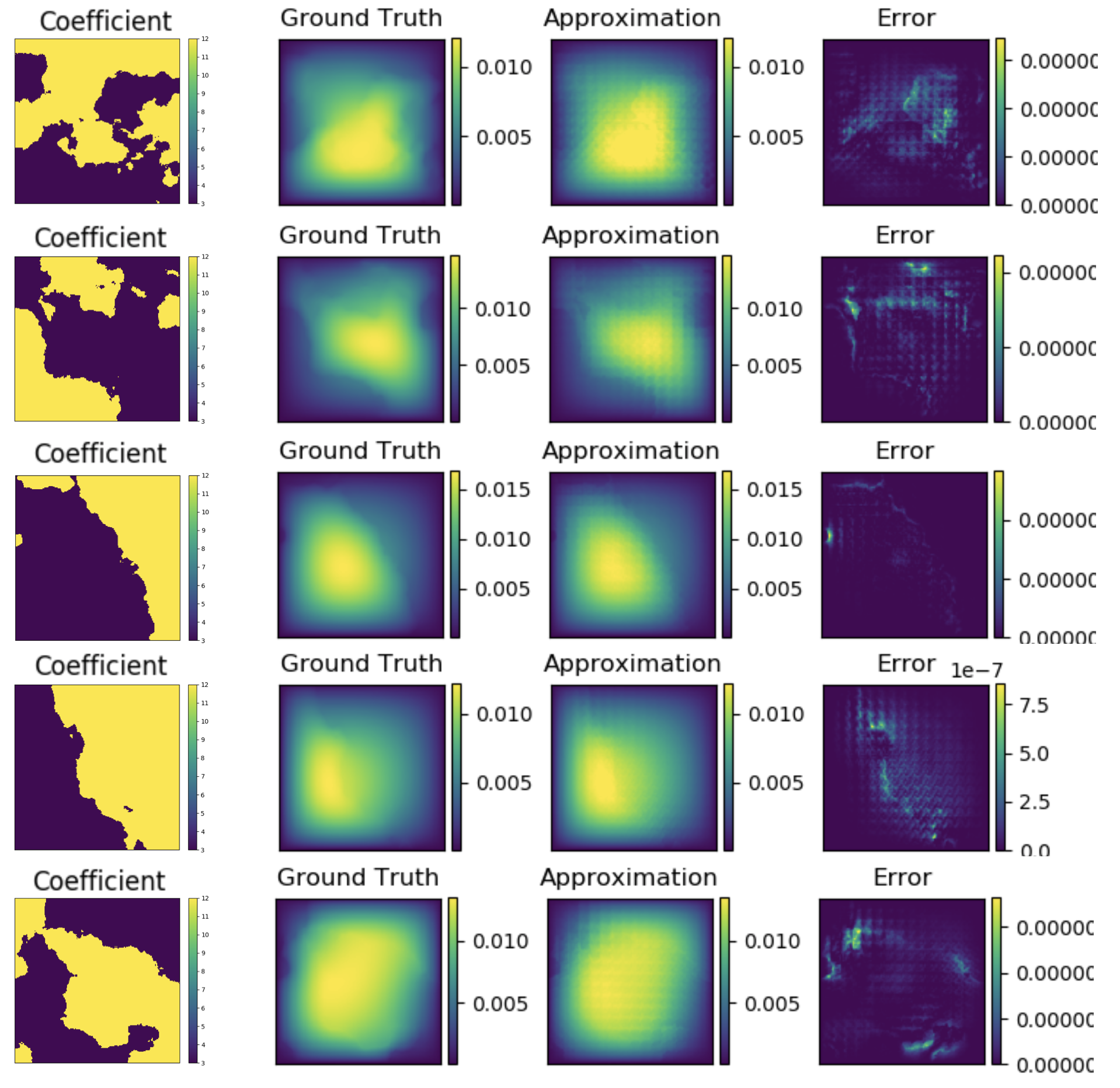
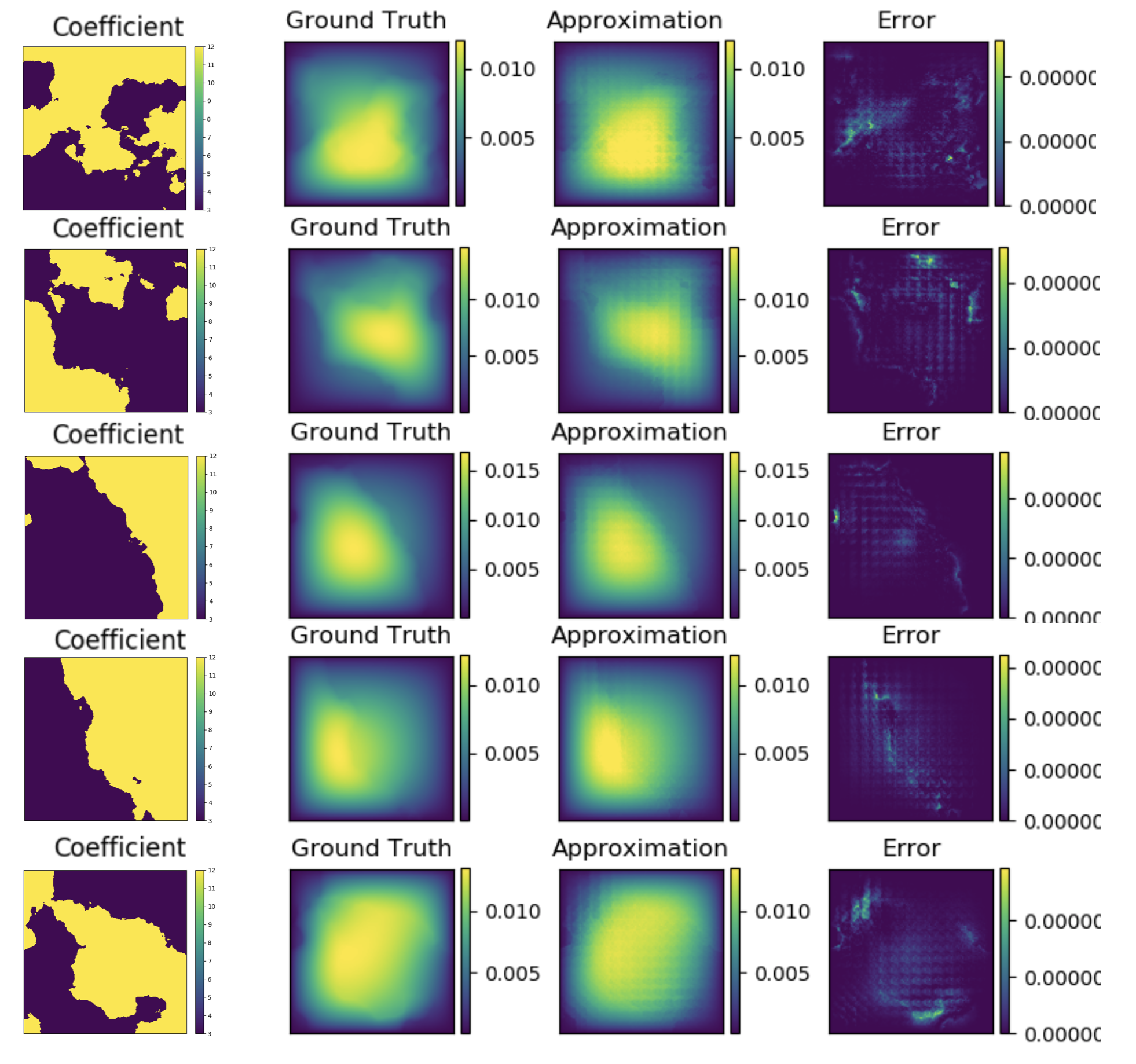
Graph kernel network for the solution of (3). It can be trained on a small resolution and will generalize to a large one. Error is point-wise squared error.
Continuous neural networks.
The concept of defining neural networks in infinite-dimensional spaces is a central problem that long been studied [Williams, 1996, Neal, 1996, Roux and Bengio, 2007, Globerson and Livni, 2016, Guss, 2016]. The general idea is to take the infinite-width limit which yields a non-parametric method and has connections to Gaussian Process Regression [Neal, 1996, Matthews et al., 2018, Garriga-Alonso et al., 2018], leading to the introduction of deep Gaussian processes [Damianou and Lawrence, 2013, Dunlop et al., 2018]. Thus far, such methods have not yielded efficient numerical algorithms that can parallel the success of convolutional or recurrent neural networks in finite dimensions in the setting of mappings between function spaces. Another idea is to simply define a sequence of compositions where each layer is a map between infinite-dimensional spaces with a finite-dimensional parametric dependence. This is the approach we take in this work, going a step further by sharing parameters between each layer.
1.2 Contributions
We introduce the concept of Neural Operator and instantiate it through graph kernel networks, a novel deep neural network method to learn the mapping between infinite-dimensional spaces of functions defined on bounded open subsets of .
-
•
Unlike existing methods, our approach is demonstrably able to learn the mapping between function spaces, and is invariant to different approximations and grids, as demonstrated in Figure 1.
-
•
We deploy the Nyström extension to connect the neural network on function space to families of GNNs on arbitrary, possibly unstructured, grids.
-
•
We demonstrate that the Neural Operator approach has competitive approximation accuracy to classical and deep learning methods.
-
•
Numerical results also show that the Neural Operator needs only to be trained on a few samples in order to generalize to the whole class of problems.
-
•
We show the ability to perform semi-supervised learning, learning from data at only a few points and then generalizing to the whole domain.
These concepts are illustrated in the context of a family of elliptic PDEs prototypical of a number of problems arising throughout the sciences and engineering.
2 PROBLEM SETTING
Our goal is to learn a mapping between two infinite dimensional spaces by using a finite collection of observations of input-output pairs from this mapping: supervised learning. Let and be separable Banach spaces and a (typically) non-linear map. Suppose we have observations where is an i.i.d. sequence from the probability measure supported on and is possibly corrupted with noise. We aim to build an approximation of by constructing a parametric map
| (2) |
for some finite-dimensional parameter space and then choosing so that .
This is a natural framework for learning in infinite-dimensions as one could define a cost functional and seek a minimizer of the problem
which directly parallels the classical finite-dimensional setting [Vapnik, 1998]. Showing the existence of minimizers, in the infinite-dimensional setting, remains a challenging open problem. We will approach this problem in the test-train setting in which empirical approximations to the cost are used. We conceptualize our methodology in the infinite-dimensional setting. This means that all finite-dimensional approximations can share a common set of network parameters which are defined in the (approximation-free) infinite-dimensional setting. To be concrete we will consider infinite-dimensional spaces which are Banach spaces of real-valued functions defined on a bounded open set in . We then consider mappings which take input functions to a PDE and map them to solutions of the PDE, both input and solutions being real-valued functions on .
A common instantiation of the preceding problem is the approximation of the second order elliptic PDE
| (3) | ||||
for some bounded, open set and a fixed function . This equation is prototypical of PDEs arising in numerous applications including hydrology [Bear and Corapcioglu, 2012] and elasticity [Antman, 2005]. For a given , equation (3) has a unique weak solution [Evans, 2010] and therefore we can define the solution operator as the map . Note that while the PDE (3) is linear, the solution operator is not.
Since our data and are , in general, functions, to work with them numerically, we assume access only to point-wise evaluations. To illustrate this, we will continue with the example of the preceding paragraph. To this end let be a -point discretization of the domain and assume we have observations , for a finite collection of input-output pairs indexed by . In the next section, we propose a kernel inspired graph neural network architecture which, while trained on the discretized data, can produce an answer for any given a new input . That is to say that our approach is independent of the discretization and therefore a true function space method; we verify this claim numerically by showing invariance of the error as . Such a property is highly desirable as it allows a transfer of solutions between different grid geometries and discretization sizes.
We note that, while the application of our methodology is based on having point-wise evaluations of the function, it is not limited by it. One may, for example, represent a function numerically as a finite set of truncated basis coefficients. Invariance of the representation would then be with respect to the size of this set. Our methodology can, in principle, be modified to accommodate this scenario through a suitably chosen architecture. We do not pursue this direction in the current work.
3 GRAPH KERNEL NETWORK
We propose a graph kernel neural network for the solution of the problem outlined in section 2. A table of notations is included in Appendix A.1. As a guiding principle for our architecture, we take the following example. Let be a differential operator depending on a parameter and consider the PDE
| (4) | ||||
for a bounded, open set and some fixed function living in an appropriate function space determined by the structure of . The elliptic operator from equation (3) is an example. Under fairly general conditions on [Evans, 2010], we may define the Green’s function as the unique solution to the problem
where is the delta measure on centered at . Note that will depend on the parameter thus we will henceforth denote it as . The solution to (4) can then be represented as
| (5) |
This is easily seen via the formal computation
Generally the Green’s function is continuous at points , for example, when is uniformly elliptic [Gilbarg and Trudinger, 2015], hence it is natural to model it via a neural network. Guided by the representation (5), we propose the following iterative architecture for .
| (6) | ||||
where is a fixed function applied element-wise, is a fixed Borel measure for each . The matrix , together with the parameters entering kernel , are to be learned from data. We model as a neural network mapping to
Discretization of the continuum picture may be viewed as replacing Borel measure by an empirical approximation based on the grid points being used. In this setting we may view as a kernel block matrix, where each entry is itself a matrix. Each block shares the same set of network parameters. This is the key to making a method that shares common parameters independent of the discretization used.
Finally, we observe that, although we have focussed on neural networks mapping to , generalizations are possible, such as mapping to , or having non-zero boundary data on and mapping to . More generally one can consider the mapping from into and use similar ideas. Indeed to illustrate ideas we will consider the mapping from to below (which is linear and for which an analytic solution is known) before moving on to study the (nonlinear) mapping from to .
Example 1: Poisson equation.
We consider a simplification of the foregoing in which we study the map from to . To this end we set , , , , , and (the Lebesgue measure) in (6). We then obtain the representation (5) with the Green’s function parameterized by the neural network with explicit dependence on , . Now consider the setting where and , so that (3) reduces to the 1-dimensional Poisson equation with explicitly computable Green’s function. Indeed,
Note that although the map is, in function space, linear, the Green’s function itself is not linear in either argument. Figure 2 shows after training with samples with periodic boundary conditions on the operator . (samples from this measure can be easily implemented by means of a random Fourier series – Karhunen-Loeve – see [Lord et al., 2014]).
Proof of concept: graph kernel network on dimensional Poisson equation; comparison of learned and truth kernel.
Example 2: 2D Poisson equation.
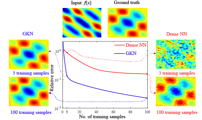
We further demonstrate the power of the graph kernel network by extending the Poisson equation studied in example 1 to the two dimensional (2D) case, where we approximate the map where . We consider two approaches: graph kernel network to approximate the 2D Green’s function and dense neural network with as input and as output such that the mapping is directly approximated.
The two neural networks are trained with the same training sets of different sizes ranging from 1 to 100 samples and tested with 1000 test samples. The relative test errors as a function of training samples are illustrated in Figure 7. We observe that the Graph kernel network approximates the map with a minimum number of training samples while still possessing a smaller test error comparing to that of a dense neural network trained with 100 samples. Therefore, the Graph kernel network potentially significantly reduces the number of required training samples to approximate the mapping. This property is especially important in practice as obtaining a huge number of training data for certain engineering/physics problems is always prohibitive.
The reason for the Graph kernel network to have such strong approximation power is because that it is able to learn the truth Green’s function for the Poisson equation, as already demonstrated in the 1D case. We shall demonstrate further in Appendix A.4 that the Graph kernel networks are apt to capture the truth kernel for the 2D Poisson equation.
Algorithmic framework.
The initialization to our network (6) can be viewed as the initial guess we make for the solution as well as any other dependence we want to make explicit. A natural choice is to start with the coefficient itself as well as the position in physical space . This -dimensional vector field is then lifted to a -dimensional vector field, an operation which we may view as the first layer of the overarching neural network. This is then used as an initialization to the kernel neural network, which is iterated times. In the final layer, we project back to the scalar field of interest with another neural network layer.
Due to the smoothing effect of the inverse elliptic operator in (3) with respect to the input data (and indeed when we consider this as input), we augment the initialization with a Gaussian smoothed version of the coefficients , together with their gradient . Thus we initialize with a -dimensional vector field. Throughout this paper the Gaussian smoothing is performed with a centred isotropic Gaussian with variance The Borel measure is chosen to be the Lebesgue measure supported on a ball at of radius . Thus we have
| (7) | ||||
| (8) | ||||
| (9) | ||||
where , , and , . The integration in (8) is approximated by a Monte Carlo sum via a message passing graph network with edge weights . The choice of measure is two-fold: 1) it allows for more efficient computation and 2) it exploits the decay property of the Green’s function. Note that if more information is known about the true kernel, it can be added into this measure. For example, if we know the true kernel has a Gaussian structure, we can define where is a Gaussian density. Then will need to learn a much less complicated function. We however do not pursue this direction in the current line of work.
Message passing graph networks.
Message passing graph networks comprise a standard architecture employing edge features [Gilmer et al., 2017]. If we properly construct the graph on the spatial domain of the PDE, the kernel integration can be viewed as an aggregation of messages. Given node features , edge features , and a graph , the message passing neural network with averaging aggregation is
| (10) |
where , is the neighborhood of according to the graph, is a neural network taking as input edge features and as output a matrix in . Relating to (8), .
Graph construction.
To use the message passing framework (10), we need to design a graph that connects the physical domain of the PDE. The nodes are chosen to be the discretized spatial locations. Here we work on a standard uniform mesh, but there are many other possibilities such as finite-element triangulations and random points at which data is acquired. The edge connectivity is then chosen according to the integration measure in (8), namely Lebesgue restricted to a ball. Each node is connected to nodes which lie within , defining the neighborhood set . Then for each neighbor , we assign the edge weight . Equation (10) can then be viewed as a Monte Carlo approximation of (8). This local structure allows for more efficient computation while remaining invariant to mesh-refinement. Indeed, since the radius parameter is chosen in physical space, the size of the set grows as the discretization size grows. This is a key feature that makes our methodology mesh-independent.
Nyström approximation of the kernel.
While the aforementioned graph structure severely reduces the computational overhead of integrating over the entire domain (corresponding to a fully-connected graph), the number of edges still scales like . To overcome this, we employ a random Nyström-type approximation of the kernel. In particular, we uniformly sample nodes from the original graph, constructing a new random sub-graph. This process is repeated times, yielding random sub-graphs each with nodes. This can be thought of as a way of reducing the variance in the estimator. We use these sub-graphs when evaluating (10) during training, leading to the more favorable scaling . Indeed, numerically we find that and is sufficient even when . In the evaluation phase, when we want the solution on a particular mesh geometry, we simply partition the mesh into sub-graphs each with nodes and evaluate each separately.
We will now highlight the quality of this kernel approximation in a RHKS setting. A real Reproducing Kernel Hilbert Space (RKHS) is a Hilbert space of functions where point-wise evaluation is a continuous linear functional, i.e. for some constant , independent of . For every RHKS, there exists a unique, symmetric, positive definite kernel , which gives the representation . Let be a linear operator on acting via the kernel
Let be its -point empirical approximation
so that
The error of this approximation achieves the Monte Carlo rate :
Proposition 1.
Suppose then there exists a constant such that
where denotes the Hilbert-Schmidt norm on operators acting on .
For proof see Appendix A.2. With stricter assumptions similar results can also be proven with high probability [Rosasco et al., 2010].
Lemma 2.
(cite Belkin) and are Hilbert-Schmidt. Furthermore, with probability greater than
where
We note that, in our algorithm, whereas the preceding results are proven only in the setting ; nonetheless they provide useful intuition regarding the approximations used in our methodology.
4 EXPERIMENTS
In this section we illustrate the claimed properties of our methodology, and compare it to existing approaches in the literature. All experimental results concern the mapping defined by (3) with . Coefficients are generated according to where with a Neumann boundry condition on the operator . The mapping takes the value 12 on the positive part of the real line and 3 on the negative. Hence the coefficients are piecewise constant with random geometry and a fixed contrast of 4. Such constructions are prototypical of physical properties such as permeability in sub-surface flows and material microstructures in elasticity. Solutions are obtained by using a second-order finite difference scheme on a grid. Different resolutions are downsampled from this dataset.
To be concrete we set the dimension of representation (i.e. the width of graph network) to be , the number of iterations to be , to be the ReLU function, and the inner kernel network to be a layer feed-forward network with widths and ReLU activation. We use the Adam optimizer with a learning rate and train for epochs with respect to the absolute mean squared error on the normalized data unless otherwise stated. These chosen hyperparameters are not optimized and could be adapted to improve performance. We employ the message passing network from the standard Pytorch graph network library Torch-geometric [Fey and Lenssen, 2019]. All the test errors are relative errors on the original data. A table of notations for the hyper-parameters can be found in Appendix A.1. The code and data can be found at https://github.com/wumming/graph-pde.
4.1 Supervised Setting
First we consider the supervised scenario that we are given training pairs , where each and are provided on a grid ().
Generalization of resolutions on full grids.
To examine the generalization property, we train the graph kernel network on resolution and test on another resolution . We fix the radius to be , train on equation pairs and test on equation pairs.
| Resolutions | |||
|---|---|---|---|
, , relative test error
As shown in Table 1, for each row, the test errors at different resolutions remain on the same scale, illustrating the desired design feature that graph kernel networks can train on one resolution and generalize to another resolution. The test errors on the diagonal ( and ) are the smallest, which means the network has the best performance when the training grid and the test grid are the same. Interestingly, for the second row, when training on , it is easier to general to than to . This is because when generalizing to a larger grid, the support of the kernel becomes large which does not hurt the performance. But when generalizing to a smaller grid, part of the support of the kernel is lost, which causes the kernel to be inaccurate.
Expressiveness and overfitting.
We compare the training error and test error with a different number of training pairs to see if the kernel network can learn the kernel structure even with a small amount of data. We study the expressiveness of the kernel network, examining how it overfits. We fix on the grid and train with whilst employing , , epochs respectively.
| Training Size | Training Error | Test Error |
|---|---|---|
, , epochs respectively.
We see from Table 2 that the kernel network already achieves a reasonable result when , and the accuracy is competitive when . In all three cases, the test error is larger than the training error suggesting that the kernel network has enough expressiveness to overfit the training set. This overfitting is not severe as the training error will not be pushed to zero even for , after epochs.
4.2 Semi-Supervised Setting
In the semi-supervised setting, we are only given nodes sampled from a grid for each training pair, and want to evaluate on nodes sampled from an grid for each test pair. To be concrete, we set the number of sampled nodes . For each training pair, we sample twice ; for each test pair, we sample once . We train on pairs and test on pairs. The radius for both training and testing is set to .
Generalization of resolutions on sampled grids.
Similar to the first experiments, we train the graph kernel network with nodes sampled from the resolution and test on nodes sampled from the resolution.
| Resolutions | |||
|---|---|---|---|
, , ,
As shown in Table 3, for each row, the test errors on different resolutions are about the same, which means the graph kernel network can also generalize in the semi-supervised setting. Comparing the rows, large training resolutions tend to have a smaller error. When sampled from a finer grid, there are more edges because the support of the kernel is larger on the finer grid. Still, the performance is best when .
The number of examples vs the times of sampling.
Increasing the number of times we sample, , reduces the error from the Nyström approximation. By comparing different we determine which value will be sufficient. When we sample times for each equation, we get a total of sampled training pairs, Table 4.
, ,
Table 4 indicates that the larger the better, but already gives a reasonable performance. Moreover, the same order of sampled training pairs, , and , result in a similar performance. It implies that in a low training data regime, increasing improves the performance.
Different number of nodes in training and testing.
To further examine the Nyström approximation, we compare different numbers of node samples for both training and testing.
As can be seen from Table 5, in general the larger and the better. For each row, fixing , the larger the better. But for each column, when fixing , increasing may not lead to better performance. This is again due to the fact that when learning on a larger grid, the kernel network learns a kernel with larger support. When evaluating on a smaller grid, the learned kernel will be truncated to have small support, leading to an increased error. In general, will be the best choice.
The radius and the number of nodes.
The computation and storage of graph networks directly scale with the number of edges. In this experiment, we want to study the trade-off between the number of nodes and the radius when fixing the number of edges.
Error (Edges), , ,
Table 6 shows the test error with the number of edges for different and . In general, the more edges, the better. For a fixed number of edges, the performance depends more on the radius than on the number of nodes . In other words, the error of truncating the kernel locally is larger than the error from the Nyström approximation. It would be better to use larger with smaller .
Inner Kernel Network .
To find the best network structure of , we compare different combinations of width and depth. We consider three cases of : 1. a layer feed-forward network with widths , 2. a layer feed-forward network with widths , and 3. a layer feed-forward network with widths , all with ReLU activation and learning rate .
| depth | depth | depth | |
|---|---|---|---|
| width = | |||
| width = | |||
| width = | |||
| width = | |||
| width = |
, ,
As shown in Table 7, have wider and deeper network increase the expensiveness of the kernel network. The diagonal combinations , , and have better test error. Notice the wide but shallow network has very bad performance. Both its training and testing error once decreased to around th epochs, but then blow off. The learning rate is probably too high for this combination. In general, depth of with with of is a good combination of Dracy Equation dataset.
4.3 Comparison with Different Benchmarks
In the following section, we compare the Graph Kernel Network with different benchmarks on a larger dataset of training pairs computed on a grid. The network is trained and evaluated on the same full grid. The results are presented in Table 8.
-
•
NN is a simple point-wise feedforward neural network. It is mesh-free, but performs badly due to lack of neighbor information.
-
•
FCN is the state of the art neural network method based on Fully Convolution Network [Zhu and Zabaras, 2018]. It has a dominating performance for small grids . But fully convolution networks are mesh-dependent and therefore their error grows when moving to a larger grid.
-
•
PCA+NN is an instantiation of the methodology proposed in [Bhattacharya et al., 2020]: using PCA as an autoencoder on both the input and output data and interpolating the latent spaces with a neural network. The method provably obtains mesh-independent error and can learn purely from data, however the solution can only be evaluated on the same mesh as the training data.
-
•
RBM is the classical Reduced Basis Method (using a PCA basis), which is widely used in applications and provably obtains mesh-independent error [DeVore, 2014]. It has the best performance but the solutions can only be evaluated on the same mesh as the training data and one needs knowledge of the PDE to employ it.
-
•
GKN stands for our graph kernel network with and . It enjoys competitive performance against all other methods while being able to generalize to different mesh geometries. Some figures arising from GKN are included in Appendix A.3.
| Networks | ||||
|---|---|---|---|---|
| NN | ||||
| FCN | ||||
| PCA+NN | ||||
| RBM | ||||
| GKN |
5 DISCUSSION AND FUTURE WORK
We have introduced the concept of Neural Operator and instantiated it through graph kernel networks designed to approximate mappings between function spaces. They are constructed to be mesh-free and our numerical experiments demonstrate that they have the desired property of being able to train and generalize on different meshes. This is because the networks learn the mapping between infinite-dimensional function spaces, which can then be shared with approximations at various levels of discretization. A further advantage is that data may be incorporated on unstructured grids, using the Nyström approximation. We demonstrate that our method can achieve competitive performance with other mesh-free approaches developed in the numerical analysis community, and beats state-of-the-art neural network approaches on large grids, which are mesh-dependent. The methods developed in the numerical analysis community are less flexible than the approach we introduce here, relying heavily on the variational structure of divergence form elliptic PDEs. Our new mesh-free method has many applications. It has the potential to be a faster solver that learns from only sparse observations in physical space. It is the only method that can work in the semi-supervised scenario when we only have measurements on some parts of the grid. It is also the only method that can transfer between different geometries. For example, when computing the flow dynamic of many different airfoils, we can construct different graphs and train together. When learning from irregular grids and querying new locations, our method does not require any interpolation, avoid subsequently interpolation error.
Disadvantage.
Graph kernel network’s runtime and storage scale with the number of edges . While other mesh-dependent methods such as PCA+NN and RBM require only . This is somewhat inevitable, because to learn the continuous function or the kernel, we need to capture pairwise information between every two nodes, which is ; when the discretization is fixed, one just needs to capture the point-wise information, which is . Therefore training and evaluating the whole grid is costly when the grid is large. On the other hand, subsampling to ameliorate cost loses information in the data, and causes errors which make our method less competitive than PCA+NN and RBM.
Future works.
To deal with the above problem, we propose that ideas such as multi-grid and fast multipole methods [Gholami et al., 2016] may be combined with our approach to reduce complexity. In particular, a multi-grid approach will construct multi-graphs corresponding to different resolutions so that, within each graph, nodes only connect to their nearest neighbors. The number of edges then scale as instead of . The error terms from Nyström approximation and local truncation can be avoided. Another direction is to extend the framework for time-dependent PDEs. Since the graph kernel network is itself an iterative solver with the time step , it is natural to frame it as an RNN that each time step corresponds to a time step of the PDEs.
Acknowledgements
Z. Li gratefully acknowledges the financial support from the Kortschak Scholars Program. K. Azizzadenesheli is supported in part by Raytheon and Amazon Web Service. A. Anandkumar is supported in part by Bren endowed chair, DARPA PAIHR00111890035, LwLL grants, Raytheon, Microsoft, Google, Adobe faculty fellowships, and DE Logi grant. K. Bhattacharya, N. B. Kovachki, B. Liu and A. M. Stuart gratefully acknowledge the financial support of the Amy research Laboratory through the Cooperative Agreement Number W911NF-12-0022. Research was sponsored by the Army Research Laboratory and was accomplished under Cooperative Agreement Number W911NF-12-2-0022. The views and conclusions contained in this document are those of the authors and should not be interpreted as representing the official policies, either expressed or implied, of the Army Research Laboratory or the U.S. Government. The U.S. Government is authorized to reproduce and distribute reprints for Government purposes notwithstanding any copyright notation herein.
References
- [Adler and Oktem, 2017] Adler, J. and Oktem, O. (2017). Solving ill-posed inverse problems using iterative deep neural networks. Inverse Problems.
- [Alet et al., 2019] Alet, F., Jeewajee, A. K., Villalonga, M. B., Rodriguez, A., Lozano-Perez, T., and Kaelbling, L. (2019). Graph element networks: adaptive, structured computation and memory. In 36th International Conference on Machine Learning. PMLR.
- [Antman, 2005] Antman, S. S. (2005). Problems In Nonlinear Elasticity. Springer.
- [Bar and Sochen, 2019] Bar, L. and Sochen, N. (2019). Unsupervised deep learning algorithm for pde-based forward and inverse problems. arXiv preprint arXiv:1904.05417.
- [Battaglia et al., 2018] Battaglia, P. W., Hamrick, J. B., Bapst, V., Sanchez-Gonzalez, A., Zambaldi, V., Malinowski, M., Tacchetti, A., Raposo, D., Santoro, A., Faulkner, R., et al. (2018). Relational inductive biases, deep learning, and graph networks. arXiv preprint arXiv:1806.01261.
- [Bear and Corapcioglu, 2012] Bear, J. and Corapcioglu, M. Y. (2012). Fundamentals of transport phenomena in porous media. Springer Science & Business Media.
- [Belongie et al., 2002] Belongie, S., Fowlkes, C., Chung, F., and Malik, J. (2002). Spectral partitioning with indefinite kernels using the nyström extension. In European conference on computer vision. Springer.
- [Bhatnagar et al., 2019] Bhatnagar, S., Afshar, Y., Pan, S., Duraisamy, K., and Kaushik, S. (2019). Prediction of aerodynamic flow fields using convolutional neural networks. Computational Mechanics, pages 1–21.
- [Bhattacharya et al., 2020] Bhattacharya, K., Kovachki, N. B., and Stuart, A. M. (2020). Model reduction and neural networks for parametric pde(s). preprint.
- [Chen et al., 2019] Chen, C., Ye, W., Zuo, Y., Zheng, C., and Ong, S. P. (2019). Graph networks as a universal machine learning framework for molecules and crystals. Chemistry of Materials, 31(9):3564–3572.
- [Cohen and DeVore, 2015] Cohen, A. and DeVore, R. (2015). Approximation of high-dimensional parametric pdes. Acta Numerica.
- [Damianou and Lawrence, 2013] Damianou, A. and Lawrence, N. (2013). Deep gaussian processes. In Artificial Intelligence and Statistics, pages 207–215.
- [DeVore, 2014] DeVore, R. A. (2014). Chapter 3: The Theoretical Foundation of Reduced Basis Methods.
- [Dunlop et al., 2018] Dunlop, M. M., Girolami, M. A., Stuart, A. M., and Teckentrup, A. L. (2018). How deep are deep gaussian processes? The Journal of Machine Learning Research, 19(1):2100–2145.
- [E and Yu, 2018] E, W. and Yu, B. (2018). The deep ritz method: A deep learning-based numerical algorithm for solving variational problems. Communications in Mathematics and Statistics.
- [Evans, 2010] Evans, L. C. (2010). Partial Differential Equations, volume 19. American Mathematical Soc.
- [Fey and Lenssen, 2019] Fey, M. and Lenssen, J. E. (2019). Fast graph representation learning with PyTorch Geometric. In ICLR Workshop on Representation Learning.
- [Garriga-Alonso et al., 2018] Garriga-Alonso, A., Rasmussen, C. E., and Aitchison, L. (2018). Deep Convolutional Networks as shallow Gaussian Processes. arXiv e-prints, page arXiv:1808.05587.
- [Gholami et al., 2016] Gholami, A., Malhotra, D., Sundar, H., and Biros, G. (2016). Fft, fmm, or multigrid? a comparative study of state-of-the-art poisson solvers for uniform and nonuniform grids in the unit cube. SIAM Journal on Scientific Computing.
- [Gilbarg and Trudinger, 2015] Gilbarg, D. and Trudinger, N. S. (2015). Elliptic partial differential equations of second order. springer.
- [Gilmer et al., 2017] Gilmer, J., Schoenholz, S. S., Riley, P. F., Vinyals, O., and Dahl, G. E. (2017). Neural message passing for quantum chemistry. In Proceedings of the 34th International Conference on Machine Learning.
- [Globerson and Livni, 2016] Globerson, A. and Livni, R. (2016). Learning infinite-layer networks: Beyond the kernel trick. CoRR, abs/1606.05316.
- [Guo et al., 2016] Guo, X., Li, W., and Iorio, F. (2016). Convolutional neural networks for steady flow approximation. In Proceedings of the 22nd ACM SIGKDD International Conference on Knowledge Discovery and Data Mining.
- [Gurtin, 1982] Gurtin, M. E. (1982). An introduction to continuum mechanics. Academic press.
- [Guss, 2016] Guss, W. H. (2016). Deep Function Machines: Generalized Neural Networks for Topological Layer Expression. arXiv e-prints, page arXiv:1612.04799.
- [Hamilton et al., 2017] Hamilton, W., Ying, Z., and Leskovec, J. (2017). Inductive representation learning on large graphs. In Advances in neural information processing systems, pages 1024–1034.
- [Herrmann et al., 2020] Herrmann, L., Schwab, C., and Zech, J. (2020). Deep relu neural network expression rates for data-to-qoi maps in bayesian pde inversion.
- [Johnson, 2012] Johnson, C. (2012). Numerical solution of partial differential equations by the finite element method. Courier Corporation.
- [Kipf and Welling, 2016] Kipf, T. N. and Welling, M. (2016). Semi-supervised classification with graph convolutional networks. arXiv preprint arXiv:1609.02907.
- [Lord et al., 2014] Lord, G. J., Powell, C. E., and Shardlow, T. (2014). An introduction to computational stochastic PDEs, volume 50. Cambridge University Press.
- [Matthews et al., 2018] Matthews, A. G. d. G., Rowland, M., Hron, J., Turner, R. E., and Ghahramani, Z. (2018). Gaussian Process Behaviour in Wide Deep Neural Networks.
- [Murphy et al., 2018] Murphy, R. L., Srinivasan, B., Rao, V., and Ribeiro, B. (2018). Janossy pooling: Learning deep permutation-invariant functions for variable-size inputs. arXiv preprint arXiv:1811.01900.
- [Neal, 1996] Neal, R. M. (1996). Bayesian Learning for Neural Networks. Springer-Verlag.
- [Nyström, 1930] Nyström, E. J. (1930). Über die praktische auflösung von integralgleichungen mit anwendungen auf randwertaufgaben. Acta Mathematica.
- [Raissi et al., 2019] Raissi, M., Perdikaris, P., and Karniadakis, G. E. (2019). Physics-informed neural networks: A deep learning framework for solving forward and inverse problems involving nonlinear partial differential equations. Journal of Computational Physics, 378:686–707.
- [Rosasco et al., 2010] Rosasco, L., Belkin, M., and Vito, E. D. (2010). On learning with integral operators. J. Mach. Learn. Res., 11:905–934.
- [Roux and Bengio, 2007] Roux, N. L. and Bengio, Y. (2007). Continuous neural networks. In Meila, M. and Shen, X., editors, Proceedings of the Eleventh International Conference on Artificial Intelligence and Statistics.
- [Vapnik, 1998] Vapnik, V. N. (1998). Statistical Learning Theory. Wiley-Interscience.
- [Veličković et al., 2017] Veličković, P., Cucurull, G., Casanova, A., Romero, A., Lio, P., and Bengio, Y. (2017). Graph attention networks.
- [Williams, 1996] Williams, C. K. I. (1996). Computing with infinite networks. In Proceedings of the 9th International Conference on Neural Information Processing Systems, Cambridge, MA, USA. MIT Press.
- [Zhu and Zabaras, 2018] Zhu, Y. and Zabaras, N. (2018). Bayesian deep convolutional encoder–decoder networks for surrogate modeling and uncertainty quantification. Journal of Computational Physics.
Appendix A Appendix
A.1 Table of Notations
| Notation | Meaning |
|---|---|
| PDE | |
| The input coefficient functions | |
| The target solution functions | |
| The spatial domain for the PDE | |
| Points in the the spatial domain | |
| -point discretization of | |
| The operator mapping the coefficients to the solutions | |
| A probability measure where sampled from. | |
| Graph Kernel Networks | |
| The kernel maps to a matrix | |
| The parameters of the kernel network | |
| The time steps | |
| The activation function | |
| The neural network representation of | |
| A Borel measure for | |
| Gaussian smoothing of | |
| The gradients of | |
| Learnable parameters of the networks. | |
| Hyperparameters | |
| The number of training pairs | |
| The number of testing pairs | |
| The underlying resolution of training points | |
| The underlying resolution of testing points | |
| Total number of nodes in the grid | |
| The number of sampled nodes per training pair | |
| The number of sampled nodes per testing pair | |
| The times of re-sampling per training pair | |
| The times of re-sampling per testing pair | |
| The radius of the ball of kernel integration for training | |
| The radius of the ball of kernel integration for testing |
A.2 Nyström Approximation
Proof of Proposition 1.
Let be an i.i.d. sequence with . Define for any . Notice that by the reproducing property,
hence
and similarly
Define for any and for any , noting that and . Further we note that
and, by Jensen’s inequality,
hence is Hilbert-Schmidt (as is since it has finite rank). We now compute,
Setting , we now have
Applying Jensen’s inequality to the convex function gives
∎
A.3 Figures of Table 8
Figure 4, 5, and 6 show graph kernel network’s performance for the first testing examples with respectively. As can be seen in the figures, most of the error occurs around the singularity of the coefficient (where the two colors cross).
ł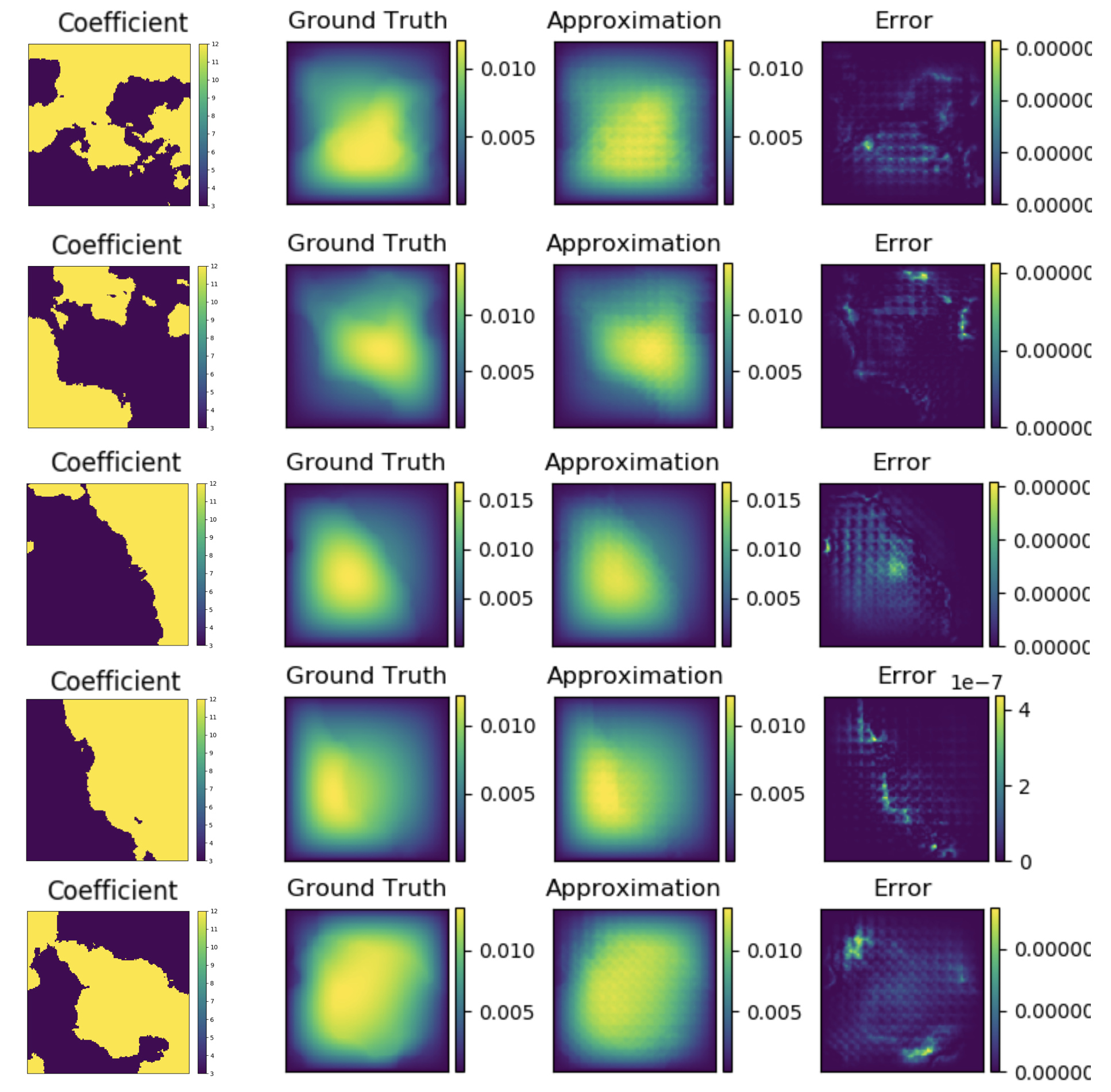
A.4 Approximating the 2D Green’s function
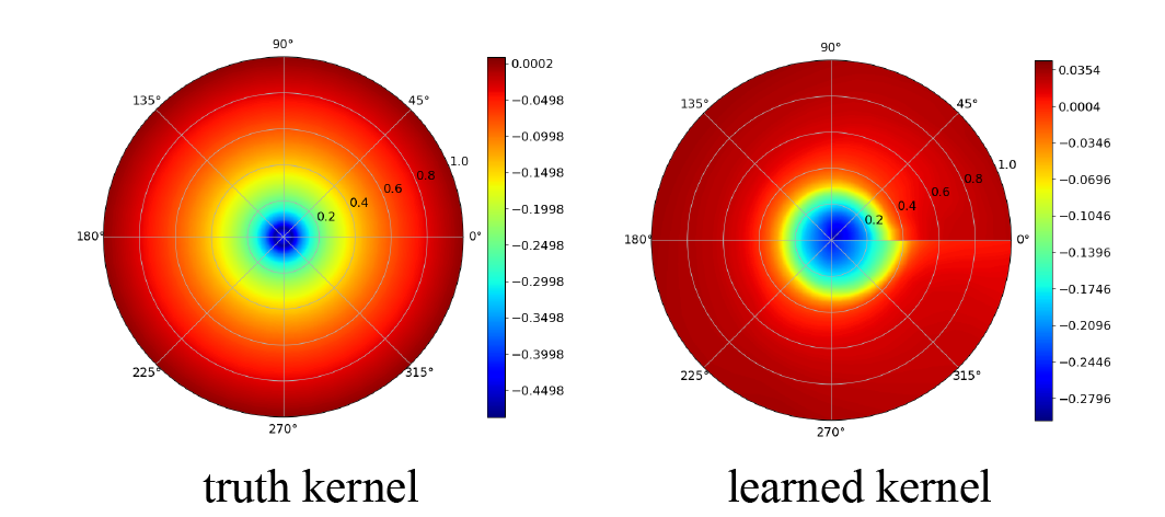
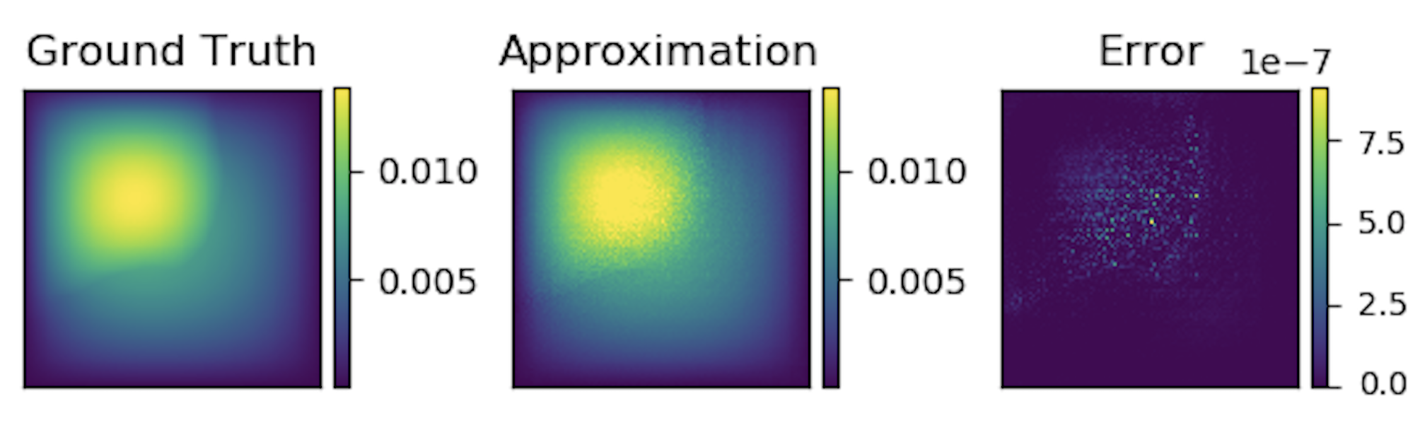
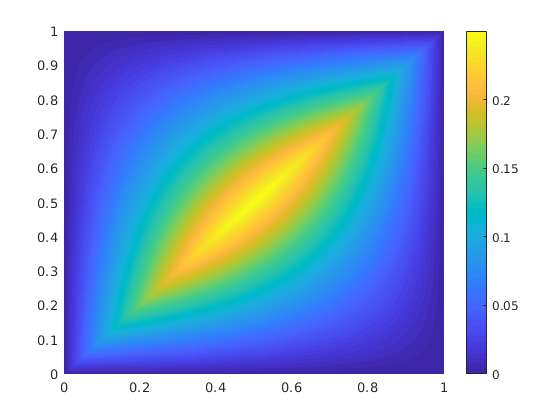
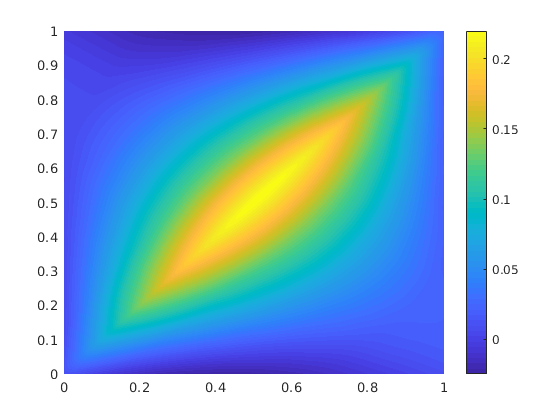
In Section 3 it has been shown that the graph kernel network is capable of approximating the truth kernel of 1D Poisson equation. Here we further demonstrate the approximation power of the graph kernel network for the 2D Poisson equation by showing that the graph kernel net work is able to capture its truth Green’s function.
Although a closed-form expression for general Green’s function of arbitrary 2D domain does not exist, it does exist when the partial differential equation is defined on a unit disk. Hence consider the 2D Poisson’s equation as introduced in Section 3 with defined on a unit disk . Recall the corresponding Green’s function in this case can be expressed in the polar coordinate as:
We first apply the graph kernel network to approximate the mapping , and then compare the learned kernel to the truth kernel . Figure 7 shows contour plots of the truth and learned Green’s function evaluated at . Again the graph kernel network is capable of learning the true Green’s function, albeit the approximating error becomes larger near the singularity at zero. As a consequence, the exceptional generalization power of the graph neural network seen in Fig. 3 is explained and expected.