Neural Tangent Kernel of Neural Networks with Loss Informed by Differential Operators

Weiye Gan, Yicheng Li, Qian Lin, Zuoqiang Shi gwy22@mails.tsinghua.edu.cn. Department of Mathematical Sciences, Tsinghua University, Beijing, China. liyc22@mails.tsinghua.edu.cn. Center for Statistical Science, Department of Industrial Engineering, Tsinghua University, Beijing, China. qianlin@tsinghua.edu.cn. Center for Statistical Science, Department of Industrial Engineering, Tsinghua University, Beijing, China. Corresponding author. zqshi@tsinghua.edu.cn. Yau Mathematical Sciences Center, Tsinghua University, Beijing, 100084, China & Yanqi Lake Beijing Institute of Mathematical Sciences and Applications, Beijing, 101408, China.

Abstract

Spectral bias is a significant phenomenon in neural network training and can be explained by neural tangent kernel (NTK) theory. In this work, we develop the NTK theory for deep neural networks with physics-informed loss, providing insights into the convergence of NTK during initialization and training, and revealing its explicit structure. We find that, in most cases, the differential operators in the loss function do not induce a faster eigenvalue decay rate and stronger spectral bias. Some experimental results are also presented to verify the theory.

Keywords: neural tangent kernel, physics-informed neural networks, spectral bias, differential operator

1 Introduction

In recent years, Physics-Informed Neural Networks (PINNs) [31] are gaining popularity as a promising alternative to solve Partial Differential Equations (PDEs). PINNs leverage the universal approximation capabilities of neural networks to approximate solutions while incorporating physical laws directly into the loss function. This approach eliminates the need for discretization and can handle high-dimensional problems more efficiently than traditional methods [14, 33]. Moreover, PINNs are mesh-free, making them particularly suitable for problems with irregular geometries [19, 39]. Despite these advantages, PINNs are not without limitations. One major challenge is their difficulty in training, often resulting in slow convergence or suboptimal solutions [6, 22]. This issue is particularly pronounced in problems with the underlying PDE solutions that contain high-frequency or multiscale features [11, 30, 40].

To explain the obstacles in training PINNs, a significant aspect is about the deficiency of neural networks in learning multifrequency functions, referred to as spectral bias [29, 38, 12, 32], which means that neural networks tend to learn the components of ”lower complexity” faster during training [29]. This phenomenon is intrinsically linked to the Neural Tangent Kernel (NTK) theory [18], as the NTK’s spectrum directly governs the convergence rates of different frequency components during training [7]. Specifically, neural networks are shown to converge faster in the directions defined by eigenfunctions of NTK with larger eigenvalues. Therefore, the components that are considered to have ”low complexity” empirically are actually eigenfunctions of NTK with large eigenvalues and vice versa for components of high complexity. The detrimental effects of spectral bias can be exacerbated by two primary factors: first, the target function inherently possesses significant components of high complexity, and second, there is a substantial disparity in the magnitudes of the NTK’s eigenvalues.

In the context of PINNs, the objective function corresponds to the solution of the PDE, rendering improvements in this aspect particularly challenging. A more promising avenue lies in refining the network architecture to ensure that the NTK exhibits a more favorable eigenvalue distribution. Several efforts have been made in this domain, such as the implementation of Fourier feature embedding [35, 20] and strategic weight balancing to harmonize the disparate components of the loss function [36].

Different from the l2 loss in standard NTK theory, PINNs generally consider the following physics informed loss

\mathcal{L}(u)=\frac{1}{2n}\sum_{i=1}^{n}(\mathcal{T}u(x_{i};\theta)-f_{i})^{2}+\frac{1}{2m}\sum_{j=1}^{m}(\mathcal{B}u(x_{j};\theta)-g_{j})^{2}

for PDE

\left\{\begin{array}[]{cc}\mathcal{D}u(x)=f(x),&x\in\Omega,\\ \mathcal{B}u(x)=g(x),&x\in\partial\Omega.\end{array}\right.

In this paper, we only focus on the loss related to the interior euqation and neglect the boundary conditions, i.e.

\mathcal{L}(u;\mathcal{T})\coloneqq\frac{1}{2n}\sum_{i=1}^{n}(\mathcal{T}u(x_{i};\theta)-f_{i})^{2}.

This loss function may be adopted when $\Omega$ is a closed manifold or the boundary conditions are already hard constraints on neural networks [8]. We first demonstrate the convergence of the neural network kernel at initialization. While most previous works only consider shallow networks. The idea based on functional analysis in [15] is applied so that we can process arbitrary high-order differential operator $\mathcal{T}$ and deep neural networks. Another benefit of this approach is that we can show that the NTK related to $\mathcal{L}(u;\mathcal{T})$ is exactly $\mathcal{T}_{x}\mathcal{T}_{x^{\prime}}K^{NT}(x,x^{\prime})$ where $K^{NT}(x,x^{\prime})$ is the NTK for l2 loss $\mathcal{L}(u;Id)$ . With this connection, we analyze the impact of $\mathcal{T}$ on the decay rate of the NTK’s eigenvalues, which affects the convergence and generalization of the related kernel regression [26, 25]. We found that the additional differential operator in the loss function does not lead to a stronger spectral bias. Therefore, to improve the performance of PINNs from a spectral bias perspective, particular attention should be paid to the equilibrium among distinct components within the loss function [36, 27]. For the convergence in training, we present a sufficient condition for general $\mathcal{T}$ and neural networks. This condition is verified in a simple but specific case. Through these results, we hope to advance the theoretical foundations of PINNs and pave the way for their broader application in scientific computing.

The remainder of the paper is organized as follows. In Section 2, we introduce the function space we consider, the settings of neural networks, and some previous results of the NTK theory. All theoretical results are demonstrated in Section 3, including the convergence of NTK during initialization and training and the impact of the differential operator within the loss on the spectrum of NTK. In Section 4, we design some experiments to verify our theory. Some conclusions are drawn in Section 5.

2 Preliminary

In this section, we introduce the basic problem setup including the function space considered and the neural network structure, as well as some background on the NTK theory.

2.1 Continuously Differential Function Spaces

Let $T\subset\mathbb{R}^{n}$ be a compact set, $k\geq 0$ be a integer and $Z_{n}$ be the $n$ -fold index set,

Z_{n}=\{\alpha=(\alpha_{1},\dots,\alpha_{n})\big{|}\alpha_{i}\text{ is a non-negative integer, }\forall i=1,\dots,n\}.

We denote $\absolutevalue{\alpha}=\sum_{i=1}^{n}\alpha_{i}$ and $D^{\alpha}=\frac{\partial^{\absolutevalue{\alpha}}}{\partial x_{1}^{\alpha_{1}}\dots\partial x_{n}^{\alpha_{n}}}$ . Then, the $k$ -times continuously differentiable function space $C^{k}(T)$ is defined as

C^{k}(T;\mathbb{R}^{m})=\{u:T\rightarrow\mathbb{R}^{m}\big{|}D^{\alpha}u\text{ is continuous on }T,\ \forall\alpha:\absolutevalue{\alpha}\leq k\}.

If $m=1$ , we disregard $\mathbb{R}^{m}$ for simplicty. The same applies to the following function spaces. $C^{k}(T;\mathbb{R}^{m})$ can be equipped with norm

\norm{u}_{C^{k}(T;\mathbb{R}^{m})}=\max_{\alpha\in Z_{n},\absolutevalue{\alpha}\leq k}\sup_{x\in T}\absolutevalue{D^{\alpha}u(x)}.

For a contant $\beta\in[0,1]$ , we also define

[u]_{C^{0,\beta}(T;\mathbb{R}^{m})}=\sup_{x,y\in T,x\neq y}\frac{\absolutevalue{u(x)-u(y)}}{\absolutevalue{x-y}^{\beta}}

and

C^{0,\beta}(T;\mathbb{R}^{m})=\{u\in C^{0}(T;\mathbb{R}^{m})\big{|}[u]_{C^{0,\beta}(T;\mathbb{R}^{m})}<\infty\},

C^{k,\beta}(T;\mathbb{R}^{m})=\{u\in C^{k}(T;\mathbb{R}^{m})\big{|}[D^{\alpha}u]_{C^{0,\beta}(T;\mathbb{R}^{m})}<\infty,\ \forall\alpha:\absolutevalue{\alpha}\leq k\}.

$C^{0,1}(T;\mathbb{R}^{m})$ is the familiar Lipschitz function space. $C^{k,\beta}(T;\mathbb{R}^{m})$ can also be equipped with norm

\norm{u}_{C^{k,\beta}(T;\mathbb{R}^{m})}=\norm{u}_{C^{k}(T;\mathbb{R}^{m})}+\max_{\alpha\in Z_{n},\absolutevalue{\alpha}\leq k}[D^{\alpha}u(x)]_{C^{0,\beta}(T;\mathbb{R}^{m})}.

For a function of two variables $u(x,x^{\prime})$ , we denote $D_{x}^{\alpha}$ as a differential operator with respect to $x$ , and similarly for $D_{x^{\prime}}^{\alpha}$ . We have analogous definitions,

C^{k\times k}(T\times T;\mathbb{R}^{m})=\{u:T\times T\rightarrow\mathbb{R}^{m}\big{|}D_{x}^{\alpha}D_{x^{\prime}}^{\alpha^{\prime}}u\text{ is continuous on }T\times T,\ \forall\alpha,\alpha^{\prime}:\absolutevalue{\alpha},\absolutevalue{\alpha^{\prime}}\leq k\}

with norm

\norm{u}_{C^{k\times k}(T\times T;\mathbb{R}^{m})}=\max_{\alpha,\alpha^{\prime}\in Z_{n},\absolutevalue{\alpha},\absolutevalue{\alpha^{\prime}}\leq k}\sup_{x,x^{\prime}\in T}\absolutevalue{D_{x}^{\alpha}D_{x^{\prime}}^{\alpha^{\prime}}u(x,x^{\prime})}

and

C^{k\times k,\beta}(T\times T;\mathbb{R}^{m})=\{u\in C^{k\times k}(T\times T;\mathbb{R}^{m})\big{|}[D_{x}^{\alpha}D_{x^{\prime}}^{\alpha^{\prime}}u]_{C^{0,\beta}(T\times T;\mathbb{R}^{m})}<\infty,\ \forall\alpha,\alpha^{\prime}:\absolutevalue{\alpha},\absolutevalue{\alpha^{\prime}}\leq k\}

with norm

\norm{u}_{C^{k\times k,\beta}(T\times T;\mathbb{R}^{m})}=\norm{u}_{C^{k\times k}(T\times T;\mathbb{R}^{m})}+\max_{\alpha,\alpha^{\prime}\in Z_{n},\absolutevalue{\alpha},\absolutevalue{\alpha^{\prime}}\leq k}[D_{x}^{\alpha}D_{x^{\prime}}^{\alpha^{\prime}}u(x)]_{C^{0,\beta}(T\times T;\mathbb{R}^{m})}.

With the chain rule and the fact that the composition of Lipschitz functions is still Lipschitz, the following lemmas can be verified.

Lemma 2.1.

Let $T_{0}\subset\mathbb{R}^{n_{0}}$ , $T_{1}\subset\mathbb{R}^{n_{1}}$ be two compact sets. Let $\varphi:T_{0}\rightarrow T_{1}$ and $\psi:T_{1}\rightarrow\mathbb{R}^{n_{2}}$ be two $C^{k,1}$ maps. Then, $\psi\circ\varphi:T_{0}\rightarrow\mathbb{R}^{n_{2}}$ is also a $C^{k,1}$ map. And there exists a constant $C$ only depending on $k$ , $\norm{\varphi}_{C^{k,1}(T_{0};T_{1})}$ and $\norm{\psi}_{C^{k,1}(T_{1};\mathbb{R}^{n_{2}})}$ such that

\norm{\psi\circ\varphi}_{C^{k,1}(T_{0};\mathbb{R}^{n_{2}})}\leq C.

Lemma 2.2.

Let $T_{0}\subset\mathbb{R}^{n_{0}}$ , $T_{1}\subset\mathbb{R}^{n_{1}}$ be two compact sets. Let $\varphi:T_{0}\times T_{0}\rightarrow T_{1}$ and $\psi:T_{1}\rightarrow\mathbb{R}^{n_{2}}$ be of class $C^{k\times k,1}$ and $C^{k,1}$ respectively. Then, $\psi\circ\varphi:T_{0}\times T_{0}\rightarrow\mathbb{R}^{n_{2}}$ is also a $C^{k\times k,1}$ map. And there exists a constant $C$ only depending on $k$ , $\norm{\varphi}_{C^{k\times k,1}(T_{0}\times T_{0};T_{1})}$ and $\norm{\psi}_{C^{k,1}(T_{1};\mathbb{R}^{n_{2}})}$ such that

\norm{\psi\circ\varphi}_{C^{k\times k,1}(T_{0}\times T_{0};\mathbb{R}^{n_{2}})}\leq C.

2.2 Settings of Neural Network

Let the input $x\in\mathcal{X}\subset\mathbb{R}^{d}$ where $\mathcal{X}$ is a convex bounded domain and the output $y\in\mathbb{R}$ . Let $m_{0}=d$ , $m_{1},\dots,m_{L}$ be the width of $L$ hidden layers and $m_{L+1}=1$ . Define the pre-activations $z^{l}(x)\in\mathbb{R}^{m_{l}}$ for $l=1,\dots,L+1$ by

\displaystyle\begin{aligned} &z^{1}(x)=W^{0}x,\\ &z^{l+1}(x)=\frac{1}{\sqrt{m_{l}}}W^{l}\sigma(z^{l}(x)),\quad\text{for }l=1,\dots,L\end{aligned}

(1)

where $W^{l}\in\mathbb{R}^{m_{l+1}\times m_{l}}$ are the weights and $\sigma$ is the activation function satisfying the following assumption for some non-negative integer.

Assumption 1.

There exists a nonnegative integer $k$ and positive constants $l_{1},\dots,l_{k}$ such that activation $\sigma\in C^{k}(\mathbb{R})$ and

\norm{\frac{\sigma^{(j)}}{1+|x|^{l_{j}}}}_{L^{\infty}}<\infty

for all $j=1,\dots,k$ .

The output of the neural network is then given by $u^{\mathrm{NN}}(x;\theta)=z^{L+1}(x)$ . Moreover, denoting by $z^{l}_{i}$ the $i$ -th component of $z^{l}$ , we have

	$\displaystyle z^{1}_{i}(x)$	$\displaystyle=\sum_{j=1}^{m_{0}}W^{0}_{ij}x_{j},$
	$\displaystyle z^{l+1}_{i}(x)$	$\displaystyle=\frac{1}{\sqrt{m_{l}}}\sum_{j=1}^{m_{l}}W^{l}_{ij}\sigma(z^{l}_{j}(x))$

We denote by $\theta=(W^{0},\dots,W^{L})$ the collection of all parameters flatten as a column vector. For simplicity, we also write $u(x)=u^{\mathrm{NN}}(x;\theta)$ . The neural network is initialized by i.i.d random variables. Specifically, all elements of $W^{l}$ are i.i.d with mean $0$ and variance $1$ .

In this paper, we consider to train neural network (1) with gradient descent and the following physics informed loss

\mathcal{L}(u;\mathcal{T})\coloneqq\frac{1}{2n}\sum_{i=1}^{n}(\mathcal{T}u(x_{i};\theta)-y_{i})^{2},

(2)

where samples $x_{i}\in\mathcal{X}$ and $\mathcal{T}$ is a known linear differential operator.

2.3 Training Dynamics

When training neural network with loss (2), the gradient flow is given by

\dot{\theta}=-\nabla_{\theta}\mathcal{L}(u;\mathcal{T})=-\frac{1}{n}\sum_{i=1}^{n}\nabla_{\theta}\mathcal{T}u(x_{i};\theta)(\mathcal{T}u(x_{i};\theta)-y_{i}).

Assuming that $u$ is sufficiently smooth, denoting $v=\mathcal{T}u$ , we have

	$\displaystyle\dot{v}$	$\displaystyle=\mathcal{T}\dot{u}=\mathcal{T}(\nabla_{\theta}u)^{T}\dot{\theta}=-[\nabla_{\theta}(\mathcal{T}u)]^{T}\nabla_{\theta}\mathcal{L}(u;\mathcal{T})$
		$\displaystyle=-\frac{1}{n}\sum_{i=1}^{n}[\nabla_{\theta}v]^{T}[\nabla_{\theta}v(x_{i};\theta)][v(x_{i};\theta)-y_{i}].$

Define the time-varying neural network kernel (NNK)

K_{\mathcal{T},\theta}(x,x^{\prime})=\left\langle{\nabla_{\theta}(\mathcal{T}u)(x;\theta),~{}\nabla_{\theta}(\mathcal{T}u)(x^{\prime};\theta)}\right\rangle=\left\langle{\nabla_{\theta}v(x;\theta),~{}\nabla_{\theta}v(x^{\prime};\theta)}\right\rangle.

(3)

Then the gradient flow of $v$ is just

\dot{v}=-\frac{1}{n}K_{\mathcal{T},\theta}(x,X)(v(X;\theta)-Y).

(4)

NTK theory suggests that this training dynamic of $v$ is very similar to that of kernel regression when neural network is wide enough. And $K_{\mathcal{T},\theta}(x,x^{\prime})$ is expected to converge to a time-invariant kernel $K_{\mathcal{T}}(x,x^{\prime})$ as width $m$ tends to infinity. If this assertion is true, we can consider the approximate kernel gradient flow of $v^{\mathrm{NTK}}$ by

\dot{v}^{\mathrm{NTK}}(x)=-\frac{1}{n}K_{\mathcal{T}}^{\mathrm{NT}}(x,X)(v^{\mathrm{NTK}}(X;\theta)-Y),

(5)

where the initialization $v^{\mathrm{NTK}}_{0}$ is not necessarily identically zero. This gradient flow can be solved explicitly by

v^{\mathrm{NTK}}(x)=v^{\mathrm{NTK}}_{0}(x)+K_{\mathcal{T}}^{\mathrm{NT}}(x,X)\varphi^{\mathrm{GF}}_{t}\left(\frac{1}{n}K_{\mathcal{T}}(X,X)\right)(Y-v^{\mathrm{NTK}}_{0}(X)),

where $\varphi^{\mathrm{GF}}_{t}(z)\coloneqq(1-e^{-tz})/z$ .

2.4 NTK Theory

When $\mathcal{T}$ in (2) is the identity map (denoted by $Id$ ), the training dynamic (4) has been widely studied with the NTK theory [18]. This theory describes the evolution of neural networks during training in the infinite-width limit, providing insight into their convergence and generalization properties. It shows that the training dynamics of neural networks under gradient descent can be approximated by a kernel method defined by the inner product of the network’s gradients. This theory has spurred extensive research, including studies on the convergence of neural networks with kernel dynamics [4, 2, 9, 24, 1], the properties of the NTK [13, 5, 26], and its statistical performance [2, 17, 23]. By bridging the empirical behavior of neural networks with their theoretical foundations, the NTK provides a framework for understanding gradient descent dynamics in function space. In this section, we review some existing conclusions that are significant in deriving our results.

The random feature and neural tangent kernel

For the finite-width neural network (1), let us define the random feature kernel $K^{\mathrm{RF},m}_{l}$ and the neural tangent kernel $K^{\mathrm{NT},\theta}_{l}$ for $l=1,\dots,L+1$ by

	$\displaystyle K^{\mathrm{RF},m}_{l}(x,x^{\prime})$	$\displaystyle=\mathrm{Cov}\left(z^{l}(x),z^{l}(x^{\prime})\right),$
	$\displaystyle K^{\mathrm{NT},\theta}_{l,ij}(x,x^{\prime})$	$\displaystyle=\left\langle{\nabla_{\theta}z^{l}_{i}(x),\nabla_{\theta}z^{l}_{j}(x^{\prime})}\right\rangle,\mbox{\quad for\quad}i,j=1,\dots,m_{l}.$

Note here that $K^{\mathrm{RF},m}_{l}$ is deterministic and $K^{\mathrm{NT},\theta}_{l}$ is random. Since $m_{l+1}=1$ , we denote $K^{\mathrm{NT},\theta}_{L+1}(x,x^{\prime})=K^{\mathrm{NT},\theta}_{L+1,11}(x,x^{\prime})$ .

Moreover, for the kernels associated with the infinite-width limit of the neural network, let us define

\displaystyle K^{\mathrm{RF}}_{1}(x,x^{\prime})=K^{\mathrm{NT}}_{1}(x,x^{\prime})=\left\langle{x,x^{\prime}}\right\rangle.

and the recurrence formula for $l=2,\dots,L+1$ ,

\displaystyle\begin{aligned} K^{\mathrm{RF}}_{l}(x,x^{\prime})&=\mathbb{E}_{(u,v)\sim N(\bm{0},\bm{B}_{l-1}(x,x^{\prime}))}\left[\sigma(u)\sigma(v)\right],\\ K^{\mathrm{NT}}_{l}(x,x^{\prime})&=K^{\mathrm{RF}}_{l}(x,x^{\prime})+K^{\mathrm{NT}}_{l-1}(x,x^{\prime})\mathbb{E}_{(u,v)\sim N(\bm{0},\bm{B}_{l-1}(x,x^{\prime}))}\left[\sigma^{(1)}(u)\sigma^{(1)}(v)\right],\end{aligned}

(6)

where the matrix $\bm{B}_{l-1}(x,x^{\prime})\in\mathbb{R}^{2\times 2}$ is defined as:

\bm{B}_{l-1}(x,x^{\prime})=\begin{pmatrix}K^{\mathrm{RF}}_{l-1}(x,x)&K^{\mathrm{RF}}_{l-1}(x,x^{\prime})\\ K^{\mathrm{RF}}_{l-1}(x,x^{\prime})&K^{\mathrm{RF}}_{l-1}(x^{\prime},x^{\prime}).\end{pmatrix}

The smoothness of the kernel $K_{l}^{\mathrm{RF}}$ and $K_{l}^{\mathrm{NT}}$ can be derived by the regularity of the activation function $\sigma$ . The proof is presented in Section A.

Lemma 2.3.

Let $k\geq 1$ be an integer and $\sigma$ satisfies Assumption 1 for $k$ . Then the kernel $K_{l}^{\mathrm{RF}}$ and $K_{l}^{\mathrm{NT}}$ defined as (6) is of classes $C^{k\times k}$ and $C^{(k-1)\times(k-1)}$ respectively.

Convergnce of NNK

The most basic and vital conclusion for NTK is that NNK defined as (3) converges to a time-invariant kernel when the width of the neural network tends to infinity.

Lemma 2.4 (Proposition 34 in [26]).

Consider NNK $K_{\mathcal{T},\theta}$ defined as (3) where $\mathcal{T}\equiv Id$ is the identity map. Let $\delta\in(0,1)$ . Under proper assumptions on the parameters $\theta_{t}$ , there exists constants $C_{1}>0$ and $C_{2}\geq 1$ such that, with probability at least $1-\delta$ ,

\sup_{t\geq 0}\absolutevalue{K_{Id,\theta_{t}}(z,z^{\prime})-K_{Id}^{\mathrm{NT}}(x,x^{\prime})}=O\left(m^{-\frac{1}{12}}\sqrt{\ln m}\right)

when $m\geq C_{1}\left(\ln\left(C_{2}/\delta\right)\right)^{5}$ and $\norm{z-x}_{2}$ , $\norm{z^{\prime}-x^{\prime}}_{2}\leq O(1/m)$ .

Convergence at initialization

As the width tends to infinity, it has been demonstrated that the neural network converges to a Gaussian process at initialization.

Lemma 2.5 ([15]).

Fix a compact set $T\subseteq\mathbb{R}^{n_{0}}$ . As the hidden layer width $m$ tends to infinity, the sequence of stochastic processes $x\mapsto u^{\mathrm{NN}}(x;\theta)$ converges weakly in $C^{0}(T)$ to a centered Gaussian process with covariance function $K^{\mathrm{RF}}_{L}$ .

3 Main Results

In this section, we present our main results. We first establish a general theorem concerning the convergence of NTKs at initialization. A sufficient condition for convergence in training is proposed and validated in some simple cases. Finally, leveraging the aforementioned results, we examine the impact of differential operators within the loss function on the spectral properties of the NTK.

3.1 Convergence at initialization

Let $S$ be a metric space and $X,X^{n},~{}n\geq 1$ be random variables taking values in $S$ . We recall that $X^{n}$ converges weakly to $X$ in $S$ , denoted by $X^{n}\xrightarrow{w}X$ , iff

\displaystyle\mathbb{E}f(X^{n})\to\mathbb{E}f(X)\mbox{\quad for any continuous bounded function\quad}f:S\to\mathbb{R}.

The first result is to show that if the activation function has a higher regularity, we can generalize Lemma 2.4 to the case of weak convergence in $C^{k}$ .

Theorem 3.1 (Convergence of initial function).

Let $T\subset\mathcal{X}$ be a compact set. $k\geq 0$ is an integer. $\sigma$ satisfies Assumption 1 for $k$ . For any $\alpha$ satisfying $|\alpha|\leq k$ , fixed $l=2,\dots,L+1$ , fixing $m_{l}$ , as $m_{1},\dots,m_{l-1}\to\infty$ , the random process

\displaystyle x\in\mathcal{X}\mapsto D^{\alpha}z^{l}(x)\in\mathbb{R}^{m_{l}}

converge weakly in $C^{0}(T;\mathbb{R}^{m_{l}})$ to a Gaussian process in $\mathbb{R}^{m_{l}}$ whose components are i.i.d. and have mean zero and covariance kernel $D_{x}^{\alpha}D_{x^{\prime}}^{\alpha}K^{\mathrm{RF}}_{l}(x,x^{\prime})$ .

Proof.

With Lemma B.1, Lemma B.5 and Proposition 2.1 in [15], we obtain the conclusion. ∎

With the aid of Theorem 3.1, the uniform convergence of NNK at initialization is demonstrated as follows.

Theorem 3.2.

Let $T\subset\mathcal{X}$ be a convex compact set. $k\geq 0$ is an integer. $\sigma$ satisfies Assumption 1 for $k+2$ . For any $\alpha,\beta$ satisfying $|\alpha|,|\beta|\leq k$ , fixed $l=2,\dots,L+1$ , fixing $m_{l}$ , as $m_{1},\dots,m_{l-1}\to\infty$ sequentially, we have

\displaystyle D_{x}^{\alpha}D_{x^{\prime}}^{\beta}K^{\mathrm{NT},\theta}_{l,ij}(x,x^{\prime})\xrightarrow{p}\delta_{ij}D_{x}^{\alpha}D_{x^{\prime}}^{\beta}K^{\mathrm{NT}}_{l}(x,x^{\prime})\mbox{\quad for\quad}i,j=1,\dots,m_{l}

(7)

under $C^{0}(T\times T;\mathbb{R}).$

Proof.

The proof is completed by induction. When $l=1$ , for any $i,j=1,\dots,m_{1}$ ,

	$\displaystyle\quad K_{1,ij}^{\mathrm{NT},\theta}(x,x^{\prime})$	$\displaystyle=\left\langle{\nabla_{\theta}z_{i}^{1}(x),\nabla_{\theta}z_{j}^{1}(x^{\prime})}\right\rangle$
		$\displaystyle=\left\langle{\nabla_{\theta}W_{i}^{0}x,\nabla_{\theta}W_{j}^{0}x^{\prime}}\right\rangle$
		$\displaystyle=\delta_{ij}\left\langle{x,x^{\prime}}\right\rangle$
		$\displaystyle=\delta_{ij}K_{1}^{\mathrm{NT}}(x,x^{\prime}).$

Suppose that as $m_{1},\dots,m_{l-1}\to\infty$ , we have

K^{\mathrm{NT},\theta}_{l,ij}(x,x^{\prime})\xrightarrow{p}\delta_{ij}K^{\mathrm{NT}}_{l}(x,x^{\prime})\mbox{\quad under\quad}C^{k\times k}(T\times T;\mathbb{R})\mbox{\quad for\quad}i,j=1,\dots,m_{l}.

For any $i,j=1,\dots,m_{l+1}$ ,

		$\displaystyle\quad K_{l+1,ij}^{\mathrm{NT},\theta}(x,x^{\prime})$		(8)
		$\displaystyle=\left\langle{\nabla_{\theta}z_{i}^{l+1}(x),\nabla_{\theta}z_{j}^{l+1}(x^{\prime})}\right\rangle$
		$\displaystyle=\delta_{ij}\frac{1}{m_{l}}\sum_{q=1}^{m_{l}}\sigma(z_{q}^{l}(x))\sigma(z_{q}^{l}(x^{\prime}))$
		$\displaystyle+\frac{1}{m_{l}}\sum_{q_{1}=1}^{m_{l}}\sum_{q_{2}=1}^{m_{l}}W_{iq_{1}}^{l}W_{jq_{2}}^{l}\sigma^{(1)}(z_{q_{1}}^{l}(x))\sigma^{(1)}(z_{q_{2}}^{l}(x^{\prime}))K_{l,q_{1}q_{2}}^{\mathrm{NT},\theta}(x,x^{\prime}).$

With the induction hypothesis and Theorem 3.1, for any fixed $m_{l}$ , as $m_{1},\dots,m_{l-1}\to\infty$ sequentially,

	$\displaystyle K_{l+1,ij}^{\mathrm{NT},\theta}(x,x^{\prime})$	$\displaystyle\xrightarrow{w}\frac{\delta_{ij}}{m_{l}}\sum_{q=1}^{m_{l}}\sigma(G_{q}^{l}(x))\sigma(G_{q}^{l}(x^{\prime}))$
		$\displaystyle+\frac{K^{\mathrm{NT}}_{l}(x,x^{\prime})}{m_{l}}\sum_{q=1}^{m_{l}}W_{iq}^{l}W_{jq}^{l}\sigma^{(1)}(G_{q}^{l}(x))\sigma^{(1)}(G_{q}^{l}(x^{\prime}))$

under $C^{0}(T\times T;\mathbb{R})$ where $G^{l}$ is a Gaussian process in $\mathbb{R}^{m_{l}}$ whose components are i.i.d. and have mean zero and covariance kernel $K^{\mathrm{RF}}_{l}$ . With weak law of large number, we obtain the finite-dimensional convergence

\left(K_{l+1,ij}^{\mathrm{NT},\theta}(x_{\alpha},x_{\alpha}^{\prime})\right)_{\alpha\in A}\xrightarrow{p}\left(\delta_{ij}K^{\mathrm{NT}}_{l+1}(x_{\alpha},x_{\alpha}^{\prime})\right)_{\alpha\in A}

for any finite set $\{(x_{\alpha},x_{\alpha}^{\prime})\in T\times T\big{|}\alpha\in A\}$ . What we still need to prove is that for any $\delta>0$ ,

\norm{K_{l+1,ij}^{\mathrm{NT},\theta}}_{C^{k\times k,1}(T\times T;\mathbb{R})}\leq C

for some $C$ not depending on $m_{1},m_{2},\dots,m_{l}$ with probability at least $1-\delta$ . Suppose that this control holds. Then, with the finite-dimensional convergence and Lemma B.2, we obatin the conclusion (7). Note that $T$ is convex. We have

\norm{K_{l+1,ij}^{\mathrm{NT},\theta}}_{C^{k\times k,1}(T\times T;\mathbb{R})}\leq\norm{K_{l+1,ij}^{\mathrm{NT},\theta}}_{C^{(k+1)\times(k+1)}(T\times T;\mathbb{R})}.

With the basic inequality $ab\leq\frac{1}{2}(a^{2}+b^{2})$ , assumption for $\sigma$ and Proposition B.7, we have

\displaystyle\mathbb{E}\left[\sup_{x,x^{\prime}\in T}\absolutevalue{D^{\alpha}\sigma(G_{1}^{l}(x))D^{\beta}\sigma(G_{1}^{l}(x^{\prime}))}\right]<\infty,

\displaystyle\mathbb{E}\left[\sup_{x,x^{\prime}\in T}\absolutevalue{{W_{11}^{l}}^{2}D^{\alpha}_{x}D^{\beta}_{x^{\prime}}\left\{\sigma^{(1)}(G_{1}^{l}(x))\sigma^{(1)}(G_{1}^{l}(x^{\prime}))K_{l}^{\mathrm{NT}}(x,x^{\prime})\right\}}\right]<\infty

and

\displaystyle\mathbb{E}\left[\sup_{x,x^{\prime}\in T}\absolutevalue{D^{\alpha}_{x}D^{\beta}_{x^{\prime}}\left\{\sigma^{(1)}(G_{1}^{l}(x))\sigma^{(1)}(G_{1}^{l}(x^{\prime}))K_{l}^{\mathrm{NT}}(x,x^{\prime})\right\}}^{2}\right]<\infty

for any $\alpha,\beta$ satisfying $|\alpha|,|\beta|\leq k+1$ . With the induction hypothesis and Theorem 3.1, for any $M>0$ ,

		$\displaystyle\quad\lim_{m_{1},\dots,m_{l-1}\rightarrow\infty}\sup_{m_{l}}\mathbb{E}\left[\sup_{x,x^{\prime}\in T}\absolutevalue{\frac{\delta_{ij}}{m_{l}}\sum_{q=1}^{m_{l}}D^{\alpha}\sigma(z_{q}^{l}(x))D^{\beta}\sigma(z_{q}^{l}(x^{\prime}))}\land M\right]$
		$\displaystyle\leq\lim_{m_{1},\dots,m_{l-1}\rightarrow\infty}\mathbb{E}\left[\sup_{x,x^{\prime}\in T}\absolutevalue{D^{\alpha}\sigma(z_{1}^{l}(x))D^{\beta}\sigma(z_{1}^{l}(x^{\prime}))}\land M\right]$
		$\displaystyle=\mathbb{E}\left[\sup_{x,x^{\prime}\in T}\absolutevalue{D^{\alpha}\sigma(G_{1}^{l}(x))D^{\beta}\sigma(G_{1}^{l}(x^{\prime}))}\land M\right]$
		$\displaystyle\leq\mathbb{E}\left[\sup_{x,x^{\prime}\in T}\absolutevalue{D^{\alpha}\sigma(G_{1}^{l}(x))D^{\beta}\sigma(G_{1}^{l}(x^{\prime}))}\right].$

Hence, there exists a constant $C_{1}$ not depending on $m_{1},\dots,m_{l}$ and $M$ such that

\sup_{m_{1},\dots,m_{l}}\mathbb{E}\left[\sup_{x,x^{\prime}\in T}\absolutevalue{\frac{\delta_{ij}}{m_{l}}\sum_{q=1}^{m_{l}}D^{\alpha}\sigma(z_{q}^{l}(x))D^{\beta}\sigma(z_{q}^{l}(x^{\prime}))}\land M\right]\leq C_{1}.

and

		$\displaystyle\quad\mathbb{P}\left(\sup_{x,x^{\prime}\in T}\absolutevalue{\frac{\delta_{ij}}{m_{l}}\sum_{q=1}^{m_{l}}D^{\alpha}\sigma(z_{q}^{l}(x))D^{\beta}\sigma(z_{q}^{l}(x^{\prime}))}>M\right)$
		$\displaystyle\leq\frac{1}{M}\mathbb{E}\left[\sup_{x,x^{\prime}\in T}\absolutevalue{\frac{\delta_{ij}}{m_{l}}\sum_{q=1}^{m_{l}}D^{\alpha}\sigma(z_{q}^{l}(x))D^{\beta}\sigma(z_{q}^{l}(x^{\prime}))}\land M\right]$
		$\displaystyle\leq\frac{C_{1}}{M}.$

For the second term on the right of (8), we do the decomposition,

		$\displaystyle\quad\frac{1}{m_{l}}\sum_{q_{1}=1}^{m_{l}}\sum_{q_{2}=1}^{m_{l}}W_{iq_{1}}^{l}W_{jq_{2}}^{l}\sigma^{(1)}(z_{q_{1}}^{l}(x))\sigma^{(1)}(z_{q_{2}}^{l}(x^{\prime}))K_{l,q_{1}q_{2}}^{\mathrm{NT},\theta}(x,x^{\prime})$
		$\displaystyle=\frac{1}{m_{l}}\sum_{q=1}^{m_{l}}W_{iq}^{l}W_{jq}^{l}\sigma^{(1)}(z_{q}^{l}(x))\sigma^{(1)}(z_{q}^{l}(x^{\prime}))K_{l,qq}^{\mathrm{NT},\theta}(x,x^{\prime})$
		$\displaystyle+\frac{1}{m_{l}}\sum_{q_{1}\neq q_{2}}W_{iq_{1}}^{l}W_{jq_{2}}^{l}\sigma^{(1)}(z_{q_{1}}^{l}(x))\sigma^{(1)}(z_{q_{2}}^{l}(x^{\prime}))K_{l,q_{1}q_{2}}^{\mathrm{NT},\theta}(x,x^{\prime}).$

For the terms on the right, it is similar to demonstrate that for any $\delta>0$ , there exists constants $C_{2}$ and $C_{3}$ such that

\mathbb{P}\left(\sup_{x,x^{\prime}\in T}\absolutevalue{\frac{1}{m_{l}}\sum_{q=1}^{m_{l}}W_{iq}^{l}W_{jq}^{l}D_{x}^{\alpha}D_{x^{\prime}}^{\beta}\left\{\sigma^{(1)}(z_{q}^{l}(x))\sigma^{(1)}(z_{q}^{l}(x^{\prime}))K_{l,qq}^{\mathrm{NT},\theta}(x,x^{\prime})\right\}}>C_{2}\right)\leq\delta

and

\mathbb{P}\left(\sup_{x,x^{\prime}\in T}\left\{\frac{1}{m_{l}^{2}}\sum_{q_{1}\neq q_{2}}\left(D^{\alpha}_{x}D^{\beta}_{x^{\prime}}\left\{\sigma^{(1)}(z_{q_{1}}^{l}(x))\sigma^{(1)}(z_{q_{2}}^{l}(x^{\prime}))K_{l,q_{1}q_{2}}^{\mathrm{NT},\theta}(x,x^{\prime})\right\}\right)^{2}\right\}>C_{3}\right)\leq\delta.

(9)

where $C_{2},C_{3}$ both not depneding on $m_{1},m_{2},\dots,m_{l}$ . We define a map $F:T\times T\rightarrow\mathbb{R}^{m_{l}^{2}-m_{l}}$ where the components of $F(x,x^{\prime})$ are given by

F_{q_{1}q_{2}}(x,x^{\prime})=\frac{1}{m_{l}}\sigma^{(1)}(z_{q_{1}}^{l}(x))\sigma^{(1)}(z_{q_{2}}^{l}(x^{\prime}))K_{l,q_{1}q_{2}}^{\mathrm{NT},\theta}(x,x^{\prime}).

Then, with (9), for any $\delta>0$ , there exsits a constant $C_{4}$ such that

\mathbb{P}\left(\norm{F}_{C^{(k+1)\times(k+1)}(T\times T)}\leq C_{4}\right)\geq 1-\frac{\delta}{2}.

Using Lemma B.4 for the map $\varphi:\mathbb{R}^{m_{l}^{2}-m_{l}}\rightarrow\mathbb{R}$ , $\varphi(x)=\sum_{q_{1}\neq q_{2}}W_{iq_{1}}^{l}W_{jq_{2}}^{l}x_{q_{1}q_{2}}$ and Lemma 2.2(for details, it is similar to the proof of Lemma B.5), there also exists a constant $C_{5}$ such that

		$\displaystyle\quad\mathbb{P}\left(\norm{\frac{1}{m_{l}}\sum_{q_{1}\neq q_{2}}W_{iq_{1}}^{l}W_{jq_{2}}^{l}\sigma^{(1)}(z_{q_{1}}^{l}(x))\sigma^{(1)}(z_{q_{2}}^{l}(x^{\prime}))K_{l,q_{1}q_{2}}^{\mathrm{NT},\theta}(x,x^{\prime})}_{C^{k\times k,1}(T\times T)}\geq C_{5}\right)$
		$\displaystyle=\mathbb{P}\left(\norm{\varphi\circ F(x,x^{\prime})}_{C^{k\times k,1}(T\times T)}\geq C_{5}\right)$
		$\displaystyle\geq 1-\delta.$

∎

There is no additional obstacle to generalize Theorem 3.2 to general linear differential operators.

Proposition 3.3.

Let $T\subset\mathcal{X}$ be a convex compact set. $k\geq 0$ is an integer. $\sigma$ satisfies Assumption 1 for $k+2$ . For any $\mathcal{T}=\sum_{r=1}^{p}a_{r}D^{\alpha_{r}}$ satisfying $|\alpha_{r}|\leq k$ and $a_{r}\in C^{0}(T)$ , fixed $l=2,\dots,L+1$ , fixing $m_{l}$ , as $m_{1},\dots,m_{l-1}\to\infty$ sequentially, we have

\displaystyle\mathcal{T}_{x}\mathcal{T}_{x^{\prime}}K^{\mathrm{NT},\theta}_{l,ij}(x,x^{\prime})\xrightarrow{p}\delta_{ij}\mathcal{T}_{x}\mathcal{T}_{x^{\prime}}K^{\mathrm{NT}}_{l}(x,x^{\prime})\mbox{\quad for\quad}i,j=1,\dots,m_{l}

under $C^{0}(T\times T;\mathbb{R}).$

3.2 Convergence in training

In the following, we will use $\norm{v}_{2}$ for the 2-norm of a vector and $\norm{A}_{2}$ for the Frobinuous norm of a matrix. Moreover, let us shorthand $\lambda_{0}=\lambda_{\min}(K^{\mathrm{NT}}_{\mathcal{T}}(X,X))$ . We also define $\tilde{v}^{\mathrm{NTK}}_{t}(x)$ as the NTK dynamics (5) with initialization $\tilde{v}^{\mathrm{NTK}}_{0}(x)=u^{\mathrm{NN}}_{0}(x)$ .

To control the training process, we first assume the following condition and establish the convergence in the training process. We will present in Lemma 3.8 that this condition is verified for the neural network with $l=1$ and $d=1$ , while extension to general cases is straightforward but very cumbersome.

Condition 3.4 (Continuity of the gradient).

There are a function $B(m):\mathbb{R}_{+}\to\mathbb{R}_{+}$ satisfying $B(m)\to\infty$ as $m\to\infty$ and a monotonically increasing function $\bar{\eta}(\varepsilon):\mathbb{R}_{+}\to\mathbb{R}_{+}$ such that for any $\varepsilon>0$ , when

\displaystyle\norm{W^{l}-W^{l}(0)}_{2}\leq B(m)\bar{\eta}(\varepsilon),\quad\forall l=0,\dots,L,

(10)

we have

\displaystyle\sup_{x\in\mathcal{X}}\norm{\nabla_{\theta}\mathcal{T}u^{\mathrm{NN}}(x;\theta)-\nabla_{\theta}\mathcal{T}u^{\mathrm{NN}}(x;\theta_{0})}_{2}\leq\varepsilon.

The following theorem shows the uniform approximation (over $x\in\mathcal{X}$ ) between the training dynamics of the neural network and the corresponding kernel regression under the physics informed loss. The general proof idea follows the perturbation analysis in the NTK literature [4, 3, 1, 26], as long as we regard $\mathcal{T}u^{\mathrm{NN}}(x;\theta)$ as a whole.

Theorem 3.5 (NTK training dynamics).

Suppose that $\mathcal{T}$ is a differential operator up to order $k$ , $\sigma$ satisfies Assumption 1 for $k+2$ , $\lambda_{0}>0$ and Condition 3.4 holds. Then, it holds in probability w.r.t. the randomness of the initialization that

\displaystyle\lim_{m\to\infty}\sup_{x\in\mathcal{X}}\absolutevalue{K_{\mathcal{T},\theta}^{m}(x,x)-K_{\mathcal{T},\theta_{0}}^{m}(x,x)}=0

(11)

and thus

\displaystyle\lim_{m\to\infty}\sup_{t\geq 0}\sup_{x\in\mathcal{X}}\absolutevalue{v^{\mathrm{NN}}_{t}(x)-\tilde{v}^{\mathrm{NTK}}_{t}(x)}=0.

(12)

Remark 3.6.

We remark here that the assumption $\lambda_{0}>0$ is not restrictive and is also a common assumption in the literature [2, 1]. If the kernel $K^{NT}_{\mathcal{T}}$ is strictly positive definite, this assumption is satisfied with probability one when the data is drawn from a continuous distribution.

To prove Theorem 3.5, we first show that a perturbation bound of the weights can imply a bound on the kernel function and the empirical kernel matrix.

Proposition 3.7.

Let condition Condition 3.4 hold and let $\varepsilon>0$ be arbitrary. Then, when (10) holds, we have

\displaystyle\absolutevalue{K_{\mathcal{T},\theta}^{m}(x,x^{\prime})-K_{\mathcal{T},\theta_{0}}^{m}(x,x^{\prime})}=O(\varepsilon),

(13)

and thus

\displaystyle\norm{K_{\mathcal{T},\theta}^{m}(X,X)-K_{\mathcal{T},\theta_{0}}^{m}(X,X)}_{\mathrm{op}}=O(n\varepsilon).

Proof.

We note that

\displaystyle K_{\mathcal{T},\theta}^{m}(x,x^{\prime})=\left\langle{\nabla_{\theta}\mathcal{T}u^{\mathrm{NN}}(x;\theta),\nabla_{\theta}\mathcal{T}u^{\mathrm{NN}}(x^{\prime};\theta)}\right\rangle,

so the result just follows from the fact that

	$\displaystyle\absolutevalue{\left\langle{v,v^{\prime}}\right\rangle-\left\langle{w,w^{\prime}}\right\rangle}$	$\displaystyle=\absolutevalue{\left\langle{v-w,v^{\prime}-w^{\prime}}\right\rangle+\left\langle{w,v^{\prime}-w^{\prime}}\right\rangle+\left\langle{v-w,w^{\prime}}\right\rangle}$
		$\displaystyle\leq\norm{v-w}\norm{v^{\prime}-w^{\prime}}+\norm{w}\norm{v^{\prime}-w^{\prime}}+\norm{v-w}\norm{w^{\prime}},$

where we can substitute $v=\nabla_{\theta}\mathcal{T}u^{\mathrm{NN}}(x;\theta)$ , $v^{\prime}=\nabla_{\theta}\mathcal{T}u^{\mathrm{NN}}(x^{\prime};\theta)$ , $w=\nabla_{\theta}\mathcal{T}u^{\mathrm{NN}}(x;\theta_{0})$ , $w^{\prime}=\nabla_{\theta}\mathcal{T}u^{\mathrm{NN}}(x^{\prime};\theta_{0})$ and apply the conditions. ∎

Proof of Theorem 3.5.

The proof resembles the perturbation analysis in [4] but with some modifications. Using Theorem 3.1 and Theorem 3.2, there are constants $L_{1},L_{2}$ such that the following holds at initialization with probability at least $1-\delta$ when $m$ is large enough:

		$\displaystyle\norm{v(x;\theta_{0})}_{C^{0}}\leq L_{1},$		(14)
		$\displaystyle\norm{K_{\mathcal{T},\theta_{0}}^{m}(X,X)-K^{\mathrm{NT}}_{\mathcal{T}}(X,X)}_{\mathrm{op}}\leq\lambda_{0}/4$		(15)
		$\displaystyle\sup_{x\in\mathcal{X}}\norm{\nabla_{\theta}\mathcal{T}u^{\mathrm{NN}}(x;\theta_{0})}_{2}\leq L_{2}.$		(16)

Let $\varepsilon>0$ be arbitrary. Using the (15) and also Proposition 3.7, we can choose some $\eta>0$ such that when $\norm{W^{l}(t)-W^{l}(0)}\leq\eta B(m)$ ,

\displaystyle\begin{aligned} &\norm{\nabla_{\theta}\mathcal{T}u^{\mathrm{NN}}(x;\theta_{t})-\nabla_{\theta}\mathcal{T}u^{\mathrm{NN}}(x;\theta_{0})}_{2}\leq 1,\\ &\norm{K_{\mathcal{T},\theta_{t}}^{m}(X,X)-K_{\mathcal{T},\theta_{0}}^{m}(X,X)}_{\mathrm{op}}\leq\lambda_{0}/4\\ &\sup_{x\in\mathcal{X}}\absolutevalue{K_{\mathcal{T},\theta_{t}}^{m}(x,x)-K_{\mathcal{T},\theta_{0}}^{m}(x,x)}\leq\varepsilon.\end{aligned}

(17)

Combining them with (14) and (15) , we have

\displaystyle\norm{\nabla_{\theta}\mathcal{T}u^{\mathrm{NN}}(x;\theta_{t})}_{2}\leq C_{0},

(18)

for some absolute constant $C_{0}>0$ , and

\displaystyle\lambda_{\min}(K_{\mathcal{T},\theta_{t}}^{m}(X,X))\geq\lambda_{0}/2.

(19)

Now, we define

\displaystyle T_{0}=\inf\left\{t\geq 0:\norm{W^{l}(t)-W^{l}(0)}\geq\eta B(m)~{}\text{for some}~{}l\right\}.

Then, (18) and (19) hold when $t\leq T_{0}$ .

Using the gradient flow (4), we find that

\displaystyle\dot{v}_{t}(X)=-\frac{1}{n}K_{\mathcal{T},\theta_{t}}^{m}(X,X)(v_{t}(X;\theta)-Y),

so (19) implies that

\displaystyle\norm{v_{t}(X;\theta)-Y}_{2}\leq\exp(-\frac{1}{4n}\lambda_{0}t)\norm{v_{0}(X)-Y}_{2},\mbox{\quad for\quad}t\leq T_{0}.

Furthermore, we recall the gradient flow equation for $W^{l}$ that

\displaystyle W^{l}_{t}-W^{l}_{0}=\int_{0}^{t}\frac{1}{n}\sum_{i=1}^{n}\left(\mathcal{T}u_{t}(x_{i})-y_{i}\right)\nabla_{W^{l}}\mathcal{T}u_{t}(x_{i})\differential t,

so when $t\leq T_{0}$ , for any $l$ , we have

	$\displaystyle\norm{W^{l}_{t}-W^{l}_{0}}_{2}$	$\displaystyle\leq\frac{1}{n}\sum_{i=1}^{n}\int_{0}^{t}\absolutevalue{\mathcal{T}u_{s}(x_{i})-y_{i}}\norm{\nabla_{W^{l}}\mathcal{T}u_{s}(x_{i})}_{2}\differential t$
		$\displaystyle\leq\frac{1}{n}\sum_{i=1}^{n}\sup_{s\in[0,t]}\norm{\nabla_{W^{l}}\mathcal{T}u_{s}(x_{i})}_{2}\int_{0}^{t}\absolutevalue{\mathcal{T}u_{s}(x_{i})-y_{i}}\differential t$
		$\displaystyle\leq\frac{4\norm{v_{0}(X)-Y}_{2}}{\lambda_{0}}\sum_{i=1}^{n}\sup_{s\in[0,t]}\norm{\nabla_{W^{l}}\mathcal{T}u_{s}(x_{i})}_{2}$
		$\displaystyle\leq\frac{4nC_{0}\norm{v_{0}(X)-Y}_{2}}{\lambda_{0}}$
		$\displaystyle\leq\frac{4nC_{0}\left(\norm{Y}_{2}+\sqrt{n}L\right)}{\lambda_{0}}$

where we used the (18) in the last inequality. Now, as long as $m$ is large enough that

\displaystyle\eta B(m)>\frac{4nC_{0}\left(\norm{Y}_{2}+\sqrt{n}L\right)}{\lambda_{0}},

an argument by contradiction shows that $T_{0}=\infty$ .

Now we have shown that $\norm{W^{l}(t)-W^{l}(0)}\leq\eta B(m)$ holds for all $t\geq 0$ , so the last inequality in (17) gives

\displaystyle\sup_{t\geq 0}\sup_{x\in\mathcal{X}}\absolutevalue{K_{\mathcal{T},\theta_{t}}^{m}(x,x)-K_{\mathcal{T},\theta_{0}}^{m}(x,x)}\leq\varepsilon.

Therefore, a standard perturbation analysis comparing the ODEs (4) and (5) yields the conclusion, see, e.g., Proof of Lemma F.1 in [4].

∎

In some simple cases, we can verify Condition 3.4 in a direct way.

Lemma 3.8.

Consider neural network (1) with $l=1$ and $d=1$ . Let $T\subset\mathcal{X}$ be a convex compact set, $k\geq 1$ be an integer and $\sigma$ satisfy Assumption 1 for $k+2$ . Then, for any $\delta>0$ , there exists functions $B(m)$ and $\eta(\varepsilon)$ satisfying such that with probability at least $1-\delta$ over initialization, we have

\sup_{x\in T}\norm{\nabla_{\theta}\frac{d^{k}u^{\mathrm{NN}}}{dx}(x;\theta)-\nabla_{\theta}\frac{d^{k}u^{\mathrm{NN}}}{dx}(x;\theta_{0})}_{2}\leq\varepsilon.

for any $W^{0},W^{1}$ satisfying

\norm{W^{0}-W^{0}(0)}_{2},\norm{W^{1}-W^{1}(0)}_{2}\leq B(m)\eta(\varepsilon).

Proof.

In this case, the neural network is defined as

u^{\mathrm{NN}}(x;\theta)\coloneqq z(x)=\frac{1}{\sqrt{m}}\sum_{i=1}^{m}W_{i}^{1}\sigma\left(W_{i}^{0}x\right).

Hence,

z^{(k)}(x)=\frac{1}{\sqrt{m}}\sum_{i=1}^{m}W_{i}^{1}{W_{i}^{0}}^{k}\sigma^{(k)}\left(W_{i}^{0}x\right)

and

		$\displaystyle\quad\norm{\nabla_{\theta}z^{(k)}(x;\theta)-\nabla_{\theta}z^{(k)}(x;\theta_{0})}_{2}^{2}$		(20)
		$\displaystyle\leq\frac{1}{m}\sum_{i=1}^{m}\left({W_{i}^{0}}^{k}\sigma^{(k)}\left(W_{i}^{0}x\right)-{W_{i}^{0}(0)}^{k}\sigma^{(k)}\left(W_{i}^{0}(0)x\right)\right)^{2}$
		$\displaystyle+\frac{k^{2}}{m}\sum_{i=1}^{m}\left(W_{i}^{1}{W_{i}^{0}}^{k-1}\sigma^{(k)}\left(W_{i}^{0}x\right)-W_{i}^{1}(0){W_{i}^{0}(0)}^{k-1}\sigma^{(k)}\left(W_{i}^{0}(0)x\right)\right)^{2}$
		$\displaystyle+\frac{x^{2}}{m}\sum_{i=1}^{m}\left(W_{i}^{1}{W_{i}^{0}}^{k}\sigma^{(k+1)}\left(W_{i}^{0}x\right)-W_{i}^{1}(0){W_{i}^{0}(0)}^{k}\sigma^{(k+1)}\left(W_{i}^{0}(0)x\right)\right)^{2}.$

We only need to demonstrate that for any $\delta>0$ , there exists $B(m)$ and $\eta(\varepsilon)$ such that with probability at least $1-\delta$ , we have

\sup_{x}\left\{\frac{1}{m}\sum_{i=1}^{m}\left({W_{i}^{0}}^{k}\sigma^{(k)}\left(W_{i}^{0}x\right)-{W_{i}^{0}(0)}^{k}\sigma^{(k)}\left(W_{i}^{0}(0)x\right)\right)^{2}\right\}\leq\varepsilon

for any $\varepsilon>0$ and $W^{0},W^{1}$ satisfying

\norm{W^{0}-W^{0}(0)}_{2},\norm{W^{1}-W^{1}(0)}_{2}\leq B(m)\eta(\varepsilon).

For the last two terms to the right of (20), we can draw a similar conclusion using the same method since $k$ is a fixed integer and $T$ is a compact set. In fact, we first do the decomposition,

		$\displaystyle\quad\frac{1}{m}\sum_{i=1}^{m}\left({W_{i}^{0}}^{k}\sigma^{(k)}\left(W_{i}^{0}x\right)-{W_{i}^{0}(0)}^{k}\sigma^{(k)}\left(W_{i}^{0}(0)x\right)\right)^{2}$
		$\displaystyle\leq\frac{3}{m}\sum_{i=1}^{m}\left({W_{i}^{0}}^{k}-{W_{i}^{0}}(0)^{k}\right)^{2}\left(\sigma^{(k)}\left(W_{i}^{0}x\right)-\sigma^{(k)}\left(W_{i}^{0}(0)x\right)\right)^{2}$
		$\displaystyle+\frac{3}{m}\sum_{i=1}^{m}\left({W_{i}^{0}}^{k}-{W_{i}^{0}}(0)^{k}\right)^{2}\sigma^{(k)}\left(W_{i}^{0}(0)x\right)^{2}$
		$\displaystyle+\frac{3}{m}\sum_{i=1}^{m}{W_{i}^{0}}(0)^{2k}\left(\sigma^{(k)}\left(W_{i}^{0}x\right)-\sigma^{(k)}\left(W_{i}^{0}(0)x\right)\right)^{2}$
		$\displaystyle\leq 3\left\{\frac{1}{m}\sum_{i=1}^{m}\left({W_{i}^{0}}^{k}-{W_{i}^{0}}(0)^{k}\right)^{4}\frac{1}{m}\sum_{i=1}^{m}\left(\sigma^{(k)}\left(W_{i}^{0}x\right)-\sigma^{(k)}\left(W_{i}^{0}(0)x\right)\right)^{4}\right\}^{\frac{1}{2}}$
		$\displaystyle+3\left\{\frac{1}{m}\sum_{i=1}^{m}\left({W_{i}^{0}}^{k}-{W_{i}^{0}}(0)^{k}\right)^{4}\frac{1}{m}\sum_{i=1}^{m}\sigma^{(k)}\left(W_{i}^{0}(0)x\right)^{4}\right\}^{\frac{1}{2}}$
		$\displaystyle+3\left\{\frac{1}{m}\sum_{i=1}^{m}{W_{i}^{0}}(0)^{4k}\frac{1}{m}\sum_{i=1}^{m}\left(\sigma^{(k)}\left(W_{i}^{0}x\right)-\sigma^{(k)}\left(W_{i}^{0}(0)x\right)\right)^{4}\right\}^{\frac{1}{2}}$

Note that

		$\displaystyle\quad\frac{1}{m}\sum_{i=1}^{m}\left({W_{i}^{0}}^{k}-{W_{i}^{0}}(0)^{k}\right)^{4}$
		$\displaystyle\leq\frac{k^{4}}{m}\sum_{i=1}^{m}\left({W_{i}^{0}}-{W_{i}^{0}}(0)\right)^{4}(\absolutevalue{W_{i}^{0}(0)}+\absolutevalue{{W_{i}^{0}}-{W_{i}^{0}}(0)})^{4k-4}$
		$\displaystyle\leq\frac{C_{1}(k)}{m}\sum_{i=1}^{m}\left({W_{i}^{0}}-{W_{i}^{0}}(0)\right)^{4}\absolutevalue{W_{i}^{0}(0)}^{4k-4}+\frac{C_{1}(k)}{m}\sum_{i=1}^{m}\left({W_{i}^{0}}-{W_{i}^{0}}(0)\right)^{4k}$
		$\displaystyle\leq C_{1}(k)\left\{\frac{1}{m}\sum_{i=1}^{m}\left({W_{i}^{0}}-{W_{i}^{0}}(0)\right)^{8}\frac{1}{m}\sum_{i=1}^{m}\absolutevalue{W_{i}^{0}(0)}^{8k-8}\right\}^{\frac{1}{2}}+\frac{C_{1}(k)}{m}\sum_{i=1}^{m}\left({W_{i}^{0}}-{W_{i}^{0}}(0)\right)^{4k}$
		$\displaystyle\leq C_{1}(k)\left\{\frac{1}{m}\norm{W^{0}-W^{0}(0)}_{2}^{8}\frac{1}{m}\sum_{i=1}^{m}\absolutevalue{W_{i}^{0}(0)}^{8k-8}\right\}^{\frac{1}{2}}+\frac{C_{1}(k)}{m}\norm{W^{0}-W^{0}(0)}_{2}^{4k}.$

And with Assumption 1, denoting $D\coloneqq\sup_{x\in T}|x|$ , we have

		$\displaystyle\quad\frac{1}{m}\sum_{i=1}^{m}\left(\sigma^{(k)}\left(W_{i}^{0}x\right)-\sigma^{(k)}\left(W_{i}^{0}(0)x\right)\right)^{4}$
		$\displaystyle\leq\frac{3D^{4}}{m}\sum_{i=1}^{m}\left(W_{i}^{0}-W_{i}^{0}(0)\right)^{4}\left(1+D^{l_{k+1}}\left(\absolutevalue{W_{i}^{0}-W_{i}^{0}(0)}+\absolutevalue{W_{i}^{0}(0)}\right)^{l_{k+1}}\right)^{4}$
		$\displaystyle\leq\frac{C_{2}(D,l_{k+1})}{m}\sum_{i=1}^{m}\left\{\absolutevalue{W_{i}^{0}-W_{i}^{0}(0)}^{4}+\absolutevalue{W_{i}^{0}-W_{i}^{0}(0)}^{4+4l_{k+1}}+\left(W_{i}^{0}-W_{i}^{0}(0)\right)^{4}W_{i}^{0}(0)^{4l_{k+1}}\right\}$
		$\displaystyle\leq\frac{C_{2}(D,l_{k+1})}{m}\left(\norm{W^{0}-W^{0}(0)}_{2}^{4}+\norm{W^{0}-W^{0}(0)}_{2}^{4+4l_{k+1}}\right)$
		$\displaystyle+C_{2}(D,l_{k+1})\left\{\frac{1}{m}\norm{W^{0}-W^{0}(0)}_{2}^{8}\frac{1}{m}\sum_{i=1}^{m}\absolutevalue{W_{i}^{0}(0)}^{8l_{k+1}}\right\}^{\frac{1}{2}}$

With Assumption 1, the fact that $T$ is compact and any moments of $W_{i}^{0}$ is finite, we have, for any $m$ ,

\mathbb{E}\left[\frac{1}{m}\sum_{i=1}^{m}\sigma^{(k)}\left(W_{i}^{0}(0)x\right)^{4}\right]=\mathbb{E}\left[\sigma^{(k)}\left(W_{1}^{0}(0)x\right)^{4}\right]<\infty

and similar conclusions for any summation above not depending on $W^{0}$ . Hence, for any $\delta>0$ , there exists a constant $M>0$ not depending on $m$ such that with probability at least $1-\delta$ ,

\frac{1}{m}\sum_{i=1}^{m}\sigma^{(k)}\left(W_{i}^{0}(0)x\right)^{4},\frac{1}{m}\sum_{i=1}^{m}{W_{i}^{0}}(0)^{4k},\frac{1}{m}\sum_{i=1}^{m}{W_{i}^{0}}(0)^{8k-8},\frac{1}{m}\sum_{i=1}^{m}\absolutevalue{{W_{i}^{0}}(0)}^{8l_{k+1}}\leq M.

Therefore, selecting $B(m)=m^{\frac{1}{d_{k}}}$ where $d_{k}\coloneqq\max\left\{8,4k,4+4l_{k+1}\right\}$ and $\eta(\varepsilon)$ sufficiently small, we can obtain the conclusion. ∎

Corollary 3.9.

Consider the neural network (1) with $l=1$ and $d=1$ . Let $T$ be a bounded closed interval in $\mathbb{R}$ , $\mathcal{T}$ is a differential operator up to order $k$ , $\sigma$ satisfies Assumption 1 for $k+2$ and $\lambda_{0}>0$ . Then, in probability with respect to the randomness of the initialization, we have

\displaystyle\lim_{m\to\infty}\sup_{t\geq 0}\sup_{x\in T}\absolutevalue{v^{\mathrm{NN}}_{t}(x)-\tilde{v}^{\mathrm{NTK}}_{t}(x)}=0.

3.3 Impact on the Spectrum

In the previous section, we demonstrate that the NTK related to the physics-informed loss (2) is $K_{\mathcal{T}}^{\mathrm{NT}}=\mathcal{T}_{x}\mathcal{T}_{x^{\prime}}K^{\mathrm{NT}}(x,x^{\prime})$ where $K^{\mathrm{NT}}=:K_{Id}^{\mathrm{NT}}$ is the NTK of the traditional l2 loss. In this section, we present some analysis and numerical experiments to explore the impact of differential operator $\mathcal{T}$ on the spectrum of integral operator with kernel $K_{\mathcal{T}}^{\mathrm{NT}}$ . Define $\mathcal{I}_{\mathcal{T}}:L^{2}(\mathcal{X})\rightarrow L^{2}(\mathcal{X})$ as the integral operator with kernel $K_{\mathcal{T}}^{\mathrm{NT}}$ , which means that for all $f\in L^{2}(\mathcal{X})$ ,

\mathcal{I}_{\mathcal{T}}f(x)=\int_{\mathcal{X}}\mathcal{T}_{x}\mathcal{T}_{x^{\prime}}K^{\mathrm{NT}}(x,x^{\prime})f(x^{\prime})dx^{\prime}.

Since $\mathcal{I}_{\mathcal{T}}$ is compact and self-adjoint, it has a sequence of real eigenvalues $\{\mu_{j}\}_{j=1}^{\infty}$ tending to zero. In addition, we denote $\{\lambda_{j}\}_{j=1}^{\infty}$ as the eigenvalue of $\mathcal{I}_{Id}$ . Then, the following lemma shows that for a large class of $\mathcal{T}$ , the decay rate of $\{\mu_{j}\}_{j=1}^{\infty}$ is not faster than that of $\{\lambda_{j}\}_{j=1}^{\infty}$ .

Lemma 3.10.

Suppose that $\{\mu_{j}\}_{j=1}^{\infty}>0$ . Let $\mathcal{T}|C_{0}^{\infty}(\mathcal{X})$ be symmetric, i.e.

\left\langle{\mathcal{T}u,v}\right\rangle_{L^{2}(\mathcal{X})}=\left\langle{u,\mathcal{T}v}\right\rangle_{L^{2}(\mathcal{X})}

for all $u,v\in C_{0}^{\infty}(\mathcal{X})$ and satisfy

C_{\mathcal{T}}\coloneqq\sup_{v\neq 0,v\in C_{0}^{\infty}(\mathcal{X})}\frac{\norm{v}_{L^{2}(\mathcal{X})}}{\norm{\mathcal{T}v}_{L^{2}(\mathcal{X})}}<\infty.

Then,

\sup_{j}\frac{\lambda_{j}}{\mu_{j}}\leq C_{\mathcal{T}}^{2}.

Proof.

With the definition, for all $j=1,2,\dots$ ,

\mu_{j}=\min_{\dim V=j-1}\max_{v\in V^{\perp}}\frac{\left\langle{\mathcal{I}_{\mathcal{T}}v,v}\right\rangle}{\norm{v}^{2}}.

Note that $C_{0}^{\infty}(\mathcal{X})$ is dense in $L^{2}(\mathcal{X})$ . Hence,

	$\displaystyle\mu_{j}$	$\displaystyle=\min_{\dim V=j-1}\sup_{v\in V^{\perp}\cap C_{0}^{\infty}(\mathcal{X})}\frac{\left\langle{\mathcal{I}_{\mathcal{T}}v,v}\right\rangle}{\norm{v}^{2}}$
		$\displaystyle=\min_{\dim V=j-1}\sup_{v\in V^{\perp}\cap C_{0}^{\infty}(\mathcal{X})}\frac{\left\langle{\mathcal{I}_{Id}\mathcal{T}v,\mathcal{T}v}\right\rangle}{\norm{v}^{2}}$
		$\displaystyle=:\sup_{v\in V_{j}^{\perp}\cap C_{0}^{\infty}(\mathcal{X})}\frac{\left\langle{\mathcal{I}_{Id}\mathcal{T}v,\mathcal{T}v}\right\rangle}{\norm{v}^{2}}.$

Moreover,

	$\displaystyle\lambda_{j}$	$\displaystyle=\min_{\dim V=j-1}\max_{v\in V^{\perp}}\frac{\left\langle{\mathcal{I}_{Id}v,v}\right\rangle}{\norm{v}^{2}}$
		$\displaystyle\leq\sup_{v\in(\mathcal{T}(V_{j}\cap C_{0}^{\infty}(\mathcal{X})))^{\perp}}\frac{\left\langle{\mathcal{I}_{Id}v,v}\right\rangle}{\norm{v}^{2}}$
		$\displaystyle=\sup_{v\in(V_{j}\cap C_{0}^{\infty}(\mathcal{X}))^{\perp}\cap C_{0}^{\infty}(\mathcal{X})}\frac{\left\langle{\mathcal{I}_{Id}\mathcal{T}v,\mathcal{T}v}\right\rangle}{\norm{\mathcal{T}v}^{2}}$
		$\displaystyle=\sup_{v\in V_{j}^{\perp}\cap C_{0}^{\infty}(\mathcal{X})}\frac{\left\langle{\mathcal{I}_{Id}\mathcal{T}v,\mathcal{T}v}\right\rangle}{\norm{\mathcal{T}v}^{2}}.$

Therefore,

\lambda_{j}\leq\sup_{v\in V_{j}^{\perp}\cap C_{0}^{\infty}(\mathcal{X})}\frac{\left\langle{\mathcal{I}_{Id}\mathcal{T}v,\mathcal{T}v}\right\rangle}{\norm{v}^{2}}\sup_{v\in V_{j}^{\perp}\cap C_{0}^{\infty}(\mathcal{X})}\frac{\norm{v}^{2}}{\norm{\mathcal{T}v}^{2}}\leq C_{\mathcal{T}}^{2}\mu_{j}.

∎

According to the Poincaré inequality, the gradient operator $\nabla$ fulfills the assumptions in Lemma 3.10. These assumptions also hold for a large class of elliptic operators since their smallest eigenvalues are positive (see section 6.5.1 in [10]).

4 Experiments

In this section, we present experimental results to verify our theory. Throughout the task, data $\{x_{i}\}_{i=1}^{n}$ are sampled uniformly from $[0,1]^{d}$ .

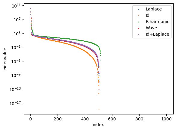
In Section 3.3, we show that the differential operator in the loss function does not make the decay rate of the eigenvalue of the integral operator related to the NTK faster. A natural inquiry arises as to whether this phenomenon persists for the NTK matrix $K_{\mathcal{T},\theta}(X,X)$ , which is closer to the neural network training dynamics (4). We employ the network structure described in (1) with depth $l=1$ and width $m=1024$ . All parameters are initialized as independent standard normal samples. Let $n=1000$ . For $d=1$ , we select $\mathcal{T}u(x)=u,\frac{\partial^{2}}{\partial x^{2}}u,u+\frac{\partial^{2}}{\partial x^{2}}u,\frac{\partial^{4}}{\partial x^{4}}u$ . For $d=2$ , we select $\mathcal{T}u(x,y)=u,\Delta u,u+\Delta u,\frac{\partial^{2}}{\partial x^{2}}u-\frac{\partial^{2}}{\partial y^{2}}u,\Delta^{2}u$ . The activation function is Tanh or $\text{ReLU}^{6}$ , i.e. $\sigma(x)=\max\{0,x\}^{6}$ . The eigenvalues of $K_{\mathcal{T},\theta}(X,X)$ at initialization are shown in Figure 1. Normalization is adopted to ensure that the largest eigenvalues are equal. A common phenomenon is that the higher the order of the differential operator $\mathcal{T}$ , the slower the decay of the eigenvalues of $K_{\mathcal{T},\theta}(X,X)$ , which aligns with our theoretical predictions.

Refer to caption — (a) $d=1,\sigma(x)=Tanh(x)$

The influence of differential operators within the loss function on the actual training process is also of considerable interest. We consider to approximate $\sin(2\pi ax)$ on $[0,1]$ with positive integer $a$ and three distinct loss functions,

		$\displaystyle\mathcal{L}_{1}(u)=\frac{1}{n}\sum_{i=1}^{n}\left(D(x_{i})u(x_{i};\theta)-\sin(2\pi ax_{i})\right)^{2},$
		$\displaystyle\mathcal{L}_{2}(u)=\frac{1}{n}\sum_{i=1}^{n}\left(-\Delta\left(D(x_{i})u(x_{i};\theta)\right)-\sin(2\pi ax_{i})\right)^{2},$
		$\displaystyle\mathcal{L}_{3}(u;w)=\frac{1-w}{n}\sum_{i=1}^{n}\left(-\Delta u(x_{i};\theta)-\sin(2\pi ax_{i})\right)^{2}+w\left(u(0;\theta)^{2}+u(1;\theta)^{2}\right)$

where $D(x)\coloneqq x(1-x)$ is a smooth distance function to ensure that $D(x)u(x;\theta)$ fulfills the homogeneous Dirichlet boundary condition [8] and $\mathcal{L}_{3}$ is the standard loss of PINNs with weight $w\in(0,1)$ . In this task, we adopt a neural network setting that is more closely aligned with scenarios in practice. The network architecture in (1) is still used, but with the addition of bias terms. The parameter initialization follows the default of nn.Linear() in Pytorch. Let $l=4$ , $m=512$ , $n=100$ and the activation function be Tanh. We employ the Adam algorithm to train the network with learning rate 1e-5 and the nomarlized loss function $\mathcal{L}_{j}(u(x;\theta))/\mathcal{L}_{j}(u(x;\theta_{0}))$ for $j=1,2,3$ . The training loss for different $a$ is shown in Figure 2. For small $a$ such as $a=0.5,1$ , the l2 loss $\mathcal{L}_{1}$ decays fastest at the beginning of the training process. As $a$ increases, the decrease rate of $\mathcal{L}_{1}$ slows down due to the constraints imposed by the spectral bias. In comparison, the loss $\mathcal{L}_{2}$ is less affected. This corroborates that the additional differential operator in the loss function does not impose a stronger spectral bias on the neural network during training. This behavior is also observed in standard PINNs with different weights $w$ .

5 Conclusion

In this paper, we develop the NTK theory for deep neural networks with physics-informed loss. We not only clarify the convergence of NTK during initialization and training, but also reveal its explicit structure. Using this structure, we prove that, in most cases, the differential operators in the loss function do not cause the neural network to face a stronger spectral bias during training. This is further supported by experiments. Therefore, if one wants to improve the performance of PINNs from the perspective of spectral bias, it may be more beneficial to focus on spectral bias caused by different terms of loss, as demonstrated in [36]. This does not mean that PINNs can better fit high-frequency functions. In fact, its training loss still decays slower when fitting a function with higher frequency, as shown in Figure 2. In instances where the solution exhibits pronounced high-frequency or multifrequency components, it is imperative to implement interventions to enhance the performance of PINNs [16, 20, 35]. It is also important to emphasize that spectral bias is merely one aspect of understanding the limitations of PINNs, and physics-informed loss has other drawbacks, such as making the optimizing problem more ill-conditioned [22]. Hence, the addition of higher-order differential operators to address the spectral bias in the loss function is not recommended.

References

[1] Zeyuan Allen-Zhu, Yuanzhi Li, and Zhao Song. A convergence theory for deep learning via over-parameterization, June 2019.
[2] Sanjeev Arora, Simon Du, Wei Hu, Zhiyuan Li, and Ruosong Wang. Fine-grained analysis of optimization and generalization for overparameterized two-layer neural networks. In International Conference on Machine Learning, pages 322–332. PMLR, 2019.
[3] Sanjeev Arora, Simon Du, Wei Hu, Zhiyuan Li, and Ruosong Wang. Fine-grained analysis of optimization and generalization for overparameterized two-layer neural networks. In International conference on machine learning, pages 322–332. PMLR, 2019.
[4] Sanjeev Arora, Simon S. Du, Wei Hu, Zhiyuan Li, Russ R Salakhutdinov, and Ruosong Wang. On exact computation with an infinitely wide neural net. In Advances in Neural Information Processing Systems, volume 32. Curran Associates, Inc., 2019.
[5] Alberto Bietti and Francis Bach. Deep equals shallow for ReLU networks in kernel regimes. arXiv preprint arXiv:2009.14397, 2020.
[6] Andrea Bonfanti, Giuseppe Bruno, and Cristina Cipriani. The challenges of the nonlinear regime for physics-informed neural networks. Advances in Neural Information Processing Systems, 37:41852–41881, 2025.
[7] Yuan Cao, Zhiying Fang, Yue Wu, Ding-Xuan Zhou, and Quanquan Gu. Towards understanding the spectral bias of deep learning. arXiv preprint arXiv:1912.01198, 2019.
[8] Jiaxin Deng, Jinran Wu, Shaotong Zhang, Weide Li, You-Gan Wang, et al. Physical informed neural networks with soft and hard boundary constraints for solving advection-diffusion equations using fourier expansions. Computers & Mathematics with Applications, 159:60–75, 2024.
[9] Simon S. Du, Xiyu Zhai, Barnabas Poczos, and Aarti Singh. Gradient descent provably optimizes over-parameterized neural networks. In International Conference on Learning Representations, September 2018.
[10] Lawrence C Evans. Partial differential equations, volume 19. American Mathematical Society, 2022.
[11] Olga Fuks and Hamdi A Tchelepi. Limitations of physics informed machine learning for nonlinear two-phase transport in porous media. Journal of Machine Learning for Modeling and Computing, 1(1), 2020.
[12] Amnon Geifman, Meirav Galun, David Jacobs, and Basri Ronen. On the spectral bias of convolutional neural tangent and gaussian process kernels. Advances in Neural Information Processing Systems, 35:11253–11265, 2022.
[13] Amnon Geifman, Abhay Yadav, Yoni Kasten, Meirav Galun, David Jacobs, and Basri Ronen. On the similarity between the Laplace and neural tangent kernels. In Advances in Neural Information Processing Systems, volume 33, pages 1451–1461, 2020.
[14] Jiequn Han, Arnulf Jentzen, and Weinan E. Solving high-dimensional partial differential equations using deep learning. Proceedings of the National Academy of Sciences, 115(34):8505–8510, 2018.
[15] Boris Hanin. Random neural networks in the infinite width limit as Gaussian processes. arXiv preprint arXiv:2107.01562, 2021.
[16] Saeid Hedayatrasa, Olga Fink, Wim Van Paepegem, and Mathias Kersemans. k-space physics-informed neural network (k-pinn) for compressed spectral mapping and efficient inversion of vibrations in thin composite laminates. Mechanical Systems and Signal Processing, 223:111920, 2025.
[17] Tianyang Hu, Wenjia Wang, Cong Lin, and Guang Cheng. Regularization matters: A nonparametric perspective on overparametrized neural network. In International Conference on Artificial Intelligence and Statistics, pages 829–837. PMLR, 2021.
[18] Arthur Jacot, Franck Gabriel, and Clement Hongler. Neural tangent kernel: Convergence and generalization in neural networks. In S. Bengio, H. Wallach, H. Larochelle, K. Grauman, N. Cesa-Bianchi, and R. Garnett, editors, Advances in Neural Information Processing Systems, volume 31. Curran Associates, Inc., 2018.
[19] Ameya D Jagtap and George Em Karniadakis. Extended physics-informed neural networks (xpinns): A generalized space-time domain decomposition based deep learning framework for nonlinear partial differential equations. Communications in Computational Physics, 28(5), 2020.
[20] Ge Jin, Jian Cheng Wong, Abhishek Gupta, Shipeng Li, and Yew-Soon Ong. Fourier warm start for physics-informed neural networks. Engineering Applications of Artificial Intelligence, 132:107887, 2024.
[21] Olav Kallenberg. Foundations of Modern Probability. Number 99 in Probability Theory and Stochastic Modelling. Springer, Cham, Switzerland, 2021.
[22] Aditi Krishnapriyan, Amir Gholami, Shandian Zhe, Robert Kirby, and Michael W Mahoney. Characterizing possible failure modes in physics-informed neural networks. Advances in neural information processing systems, 34:26548–26560, 2021.
[23] Jianfa Lai, Manyun Xu, Rui Chen, and Qian Lin. Generalization ability of wide neural networks on R, February 2023.
[24] Jaehoon Lee, Lechao Xiao, Samuel Schoenholz, Yasaman Bahri, Roman Novak, Jascha Sohl-Dickstein, and Jeffrey Pennington. Wide neural networks of any depth evolve as linear models under gradient descent. In Advances in Neural Information Processing Systems, volume 32. Curran Associates, Inc., 2019.
[25] Yicheng Li, Weiye Gan, Zuoqiang Shi, and Qian Lin. Generalization error curves for analytic spectral algorithms under power-law decay. arXiv preprint arXiv:2401.01599, 2024.
[26] Yicheng Li, Zixiong Yu, Guhan Chen, and Qian Lin. On the eigenvalue decay rates of a class of neural-network related kernel functions defined on general domains. Journal of Machine Learning Research, 25(82):1–47, 2024.
[27] Qiang Liu, Mengyu Chu, and Nils Thuerey. Config: Towards conflict-free training of physics informed neural networks. arXiv preprint arXiv:2408.11104, 2024.
[28] Athanasios Papoulis and S Unnikrishna Pillai. Probability, random variables, and stochastic processes. McGraw-Hill Europe: New York, NY, USA, 2002.
[29] Nasim Rahaman, Aristide Baratin, Devansh Arpit, Felix Draxler, Min Lin, Fred Hamprecht, Yoshua Bengio, and Aaron Courville. On the spectral bias of neural networks. In International conference on machine learning, pages 5301–5310. PMLR, 2019.
[30] Maziar Raissi. Deep hidden physics models: Deep learning of nonlinear partial differential equations. Journal of Machine Learning Research, 19(25):1–24, 2018.
[31] Maziar Raissi, Paris Perdikaris, and George E Karniadakis. Physics-informed neural networks: A deep learning framework for solving forward and inverse problems involving nonlinear partial differential equations. Journal of Computational physics, 378:686–707, 2019.
[32] Basri Ronen, David Jacobs, Yoni Kasten, and Shira Kritchman. The convergence rate of neural networks for learned functions of different frequencies. Advances in Neural Information Processing Systems, 32, 2019.
[33] Justin Sirignano and Konstantinos Spiliopoulos. Dgm: A deep learning algorithm for solving partial differential equations. Journal of computational physics, 375:1339–1364, 2018.
[34] Roman Vershynin. High-Dimensional Probability: An Introduction with Applications in Data Science, volume 47. Cambridge university press, 2018.
[35] Sifan Wang, Hanwen Wang, and Paris Perdikaris. On the eigenvector bias of fourier feature networks: From regression to solving multi-scale pdes with physics-informed neural networks. Computer Methods in Applied Mechanics and Engineering, 384:113938, 2021.
[36] Sifan Wang, Xinling Yu, and Paris Perdikaris. When and why pinns fail to train: A neural tangent kernel perspective. Journal of Computational Physics, 449:110768, 2022.
[37] Jon Wellner et al. Weak convergence and empirical processes: with applications to statistics. Springer Science & Business Media, 2013.
[38] Zhi-Qin John Xu, Yaoyu Zhang, and Yanyang Xiao. Training behavior of deep neural network in frequency domain. In Neural Information Processing: 26th International Conference, ICONIP 2019, Sydney, NSW, Australia, December 12–15, 2019, Proceedings, Part I 26, pages 264–274. Springer, 2019.
[39] Lei Yuan, Yi-Qing Ni, Xiang-Yun Deng, and Shuo Hao. A-pinn: Auxiliary physics informed neural networks for forward and inverse problems of nonlinear integro-differential equations. Journal of Computational Physics, 462:111260, 2022.
[40] Yinhao Zhu, Nicholas Zabaras, Phaedon-Stelios Koutsourelakis, and Paris Perdikaris. Physics-constrained deep learning for high-dimensional surrogate modeling and uncertainty quantification without labeled data. Journal of Computational Physics, 394:56–81, 2019.

Appendix A Smoothness of the NTK

In this section, we verify the smoothness of kernel $K^{\mathrm{RF}}_{1}$ and $K^{\mathrm{NT}}_{1}$ defined as (6). For the convenience of reader, we first recall the definition.

\displaystyle K^{\mathrm{RF}}_{1}(x,x^{\prime})=K^{\mathrm{NT}}_{1}(x,x^{\prime})=\left\langle{x,x^{\prime}}\right\rangle.

and for $l=2,\dots,L+1$ ,

	$\displaystyle K^{\mathrm{RF}}_{l}(x,x^{\prime})$	$\displaystyle=\mathbb{E}_{(u,v)\sim N(\bm{0},\bm{B}_{l-1}(x,x^{\prime}))}\left[\sigma(u)\sigma(v)\right],$
	$\displaystyle K^{\mathrm{NT}}_{l}(x,x^{\prime})$	$\displaystyle=K^{\mathrm{RF}}_{l}(x,x^{\prime})+K^{\mathrm{NT}}_{l-1}(x,x^{\prime})\mathbb{E}_{(u,v)\sim N(\bm{0},\bm{B}_{l-1}(x,x^{\prime}))}\left[\sigma^{(1)}(u)\sigma^{(1)}(v)\right],$

where the matrix $\bm{B}_{l-1}(x,x^{\prime})\in\mathbb{R}^{2\times 2}$ is defined as:

\bm{B}_{l-1}(x,x^{\prime})=\begin{pmatrix}K^{\mathrm{RF}}_{l-1}(x,x)&K^{\mathrm{RF}}_{l-1}(x,x^{\prime})\\ K^{\mathrm{RF}}_{l-1}(x,x^{\prime})&K^{\mathrm{RF}}_{l-1}(x^{\prime},x^{\prime}).\end{pmatrix}

Proposition A.1.

Let $f,g$ be two functions that $f,g,f^{\prime},g^{\prime}\in L^{2}(\mathbb{R},e^{-x^{2}/2}\differential x)$ . Denoting

\displaystyle F(\rho)=\mathbb{E}_{(u,v)\sim N(\bm{0},\bm{\Sigma})}f(u)g(v),\quad\Sigma=\begin{pmatrix}1&\rho\\ \rho&1\end{pmatrix}.

Then,

\displaystyle F^{\prime}(\rho)=\mathbb{E}_{(u,v)\sim N(\bm{0},\bm{\Sigma})}f^{\prime}(u)g^{\prime}(v).

Proof.

Denote by $h_{i}(x)$ the Hermite polynomial basis with respect to the normal distribution. Let us consider the Hermite expansion of $f,g$ :

\displaystyle f(u)=\sum_{i=0}^{\infty}\alpha_{i}h_{i}(u),\quad g(v)=\sum_{j=0}^{\infty}\beta_{j}h_{j}(v),

and also $f^{\prime},g^{\prime}$ :

\displaystyle f^{\prime}(u)=\sum_{i=0}^{\infty}\alpha_{i}^{\prime}h_{i}(u),\quad g^{\prime}(v)=\sum_{j=0}^{\infty}\beta_{j}^{\prime}h_{j}(v).

Using the fact that $h_{i}^{\prime}(u)=\sqrt{i}h_{i-1}(u)$ , we derive $\alpha_{i-1}^{\prime}=\sqrt{i}\alpha_{i}$ and $\beta_{i-1}^{\prime}=\sqrt{i}\beta_{i}$ for $i\geq 1$ .

Now, we use the fact that $\mathbb{E}h_{i}(u)h_{j}(v)=\rho^{i}\delta_{ij}$ for $(u,v)\sim N(\bm{0},\bm{\Sigma})$ to obtain

\displaystyle\mathbb{E}_{(u,v)}f(u)g(v)=\sum_{i,j}\alpha_{i}\beta_{j}\mathbb{E}h_{i}(u)h_{j}(v)=\sum_{i=0}^{\infty}\alpha_{i}\beta_{i}\rho^{i},

and thus

\displaystyle\partialderivative{\rho}\mathbb{E}_{(u,v)}f(u)g(v)=\sum_{i=0}^{\infty}i\alpha_{i}\beta_{i}\rho^{i-1}=\sum_{i=1}^{\infty}\alpha_{i-1}^{\prime}\beta_{i-1}^{\prime}\rho^{i-1}=\sum_{i=0}^{\infty}\alpha_{i}^{\prime}\beta_{i}^{\prime}\rho^{i}=\mathbb{E}_{(u,v)}f^{\prime}(u)g^{\prime}(v).

∎

Lemma A.2.

Let Assumption 1 hold for both $\sigma_{1},\sigma_{2}$ . Let us define a function $F(\bm{A})$ on positive semi-definite matrices $\bm{A}=(A_{ij})_{2\times 2}\in\mathrm{PSD}(2)$ as

F(\bm{A})=\mathbb{E}_{(u,v)\sim N(\bm{0},\bm{A})}\sigma_{1}(u)\sigma_{2}(v).

Then, denoting $\mathcal{D}=\left\{\bm{A}\in\mathrm{PSD}(2):A_{11},A_{22}\in[c^{-1},c]\right\}$ for some constant $c>1$ , we have $F(\bm{A})\in C^{k}(\mathcal{D})$ and for all $\absolutevalue{\alpha}\leq k$ ,

\absolutevalue{D^{\alpha}F(\bm{A})}\leq C,

where $C$ is a constant depending only on the constants in Assumption 1 and $c$ .

Proof.

We first prove the case for $k=1$ . Let us consider parameterizing

\displaystyle\bm{A}=\begin{pmatrix}a^{2}&\rho ab\\ \rho ab&b^{2}\end{pmatrix},

where $\rho\in[-1,1]$ and $a,b\in[c^{-1/2},c^{1/2}]$ . Then,

\displaystyle F(\bm{A})=\mathbb{E}_{(u,v)\sim N(\bm{0},\bm{B})}\sigma_{1}(au)\sigma_{2}(bv),\quad\bm{B}=\begin{pmatrix}1&\rho\\ \rho&1\end{pmatrix}.

Consequently,

\displaystyle\partialderivative{F}{a}=\mathbb{E}_{(u,v)\sim N(\bm{0},\bm{B})}\left(u\sigma_{1}^{\prime}(au)\sigma_{2}(bv)\right),\quad\partialderivative{F}{b}=\mathbb{E}_{(u,v)\sim N(\bm{0},\bm{B})}\left(v\sigma_{1}(au)\sigma_{2}^{\prime}(bv)\right).

Then, using Assumption 1, we have

\displaystyle\norm{\partialderivative{F}{a}}_{C^{0}}^{2}\leq\left[\mathbb{E}\left(u\sigma_{1}^{\prime}(au)\right)^{2}\right]\left[\mathbb{E}\left(\sigma_{2}(bv)\right)^{2}\right]\leq C

for some constant $C$ . For $\rho$ , we apply Proposition A.1 to get

\displaystyle\partialderivative{F}{\rho}=ab\mathbb{E}_{(u,v)\sim N(\bm{0},\bm{B})}\left(\sigma_{1}^{\prime}(au)\right)\left(\sigma_{2}^{\prime}(bv)\right).

Hence,

\displaystyle\absolutevalue{\partialderivative{F}{\rho}}\leq ab\left[\mathbb{E}\left(\sigma_{1}^{\prime}(au)\right)^{2}\right]^{1/2}\left[\mathbb{E}\left(\sigma_{2}^{\prime}(bv)\right)^{2}\right]^{1/2}\leq C

for some constant $C$ .

Now, using $a=\sqrt{A_{11}}$ , $b=\sqrt{A_{22}}$ and $\rho=A_{12}/\sqrt{A_{11}A_{22}}$ , it is easy to see that the partial derivatives $\partialderivative{a}{A_{ij}}$ , $\partialderivative{b}{A_{ij}}$ and $\partialderivative{\rho}{A_{ij}}$ are bounded by a constant depending only on $c$ . Applying the chain rule finishes the proof for $k=1$ .

Finally, the case of general $k$ follows by induction with $\sigma_{1},\sigma_{2}$ replaced.

∎

Proof of Lemma 2.3.

Using Lemma A.2, we see that the mappings

\displaystyle\bm{\Sigma}\mapsto\mathbb{E}_{(u,v)\sim N(\bm{0},\bm{\Sigma})}\sigma(u)\sigma(v),\quad\bm{\Sigma}\mapsto\mathbb{E}_{(u,v)\sim N(\bm{0},\bm{\Sigma})}\sigma^{\prime}(u)\sigma^{\prime}(v)

belong to class $C^{k}$ and $C^{k-1}$ respectively. Hence, the result follows by the recurrence formula and fact that compositions of $C^{k}$ mappings are still $C^{k}$ . ∎

Appendix B Auxiliary results

The following lemma gives a sufficient condition for the weak convergence in $C^{k}(T)$ .

Lemma B.1 (Convergence of $C^{k}$ processes).

Let $\mathcal{X}\subseteq\mathbb{R}^{d}$ be an open set. Let $(X^{n}_{t})_{t\in\mathcal{X}},~{}n\geq 1$ be random processes with $C^{k}(\mathcal{X})$ paths a.s. and $(X_{t})_{t\in\mathcal{X}}$ be a Gaussian field with mean zero and $C^{k\times k}$ covariance kernel. Denote by $D^{\alpha}$ the derivative with respect to $t$ for multi-index $\alpha$ . Suppose that

1.

For any $t_{1},\dots,t_{m}\in T$ , the finite dimensional convergence holds:

$\displaystyle\left(X^{n}_{t_{1}},\dots,X^{n}_{t_{m}}\right)\xrightarrow{w}\left(X_{t_{1}},\dots,X_{t_{m}}\right).$

For any $\alpha$ satisfying $|\alpha|\leq k$ and $\delta>0$ , there exists $L>0$ such that

\displaystyle\sup_{n}\mathbb{P}\left\{\sup_{t,s\in T}\frac{\absolutevalue{D^{\alpha}(X_{t}^{n}-X_{s}^{n})}}{\norm{t-s}_{2}}>L\right\}<\delta.

3.

For any $\alpha$ satisfying $|\alpha|\leq k$ and $\delta>0$ , there exists $C>0$ such that

$\displaystyle\sup_{n}\mathbb{P}\left\{\sup_{t\in T}\absolutevalue{D^{\alpha}X_{t}^{n}}>C\right\}<\delta.$

Then, for any compact set $T\subset\mathcal{X}$ and $\alpha$ satisfying $|\alpha|\leq k$ , we have

\displaystyle D^{\alpha}X^{n}_{t}\xrightarrow{w}D^{\alpha}X_{t}\mbox{\quad in\quad}C^{0}(T).

Proof.

With condition 2, 3 for $\alpha=\mathbf{0}$ and condition 1 (We refer to [21, Section 23] for more details),

X^{n}_{t}\xrightarrow{w}X_{t}\mbox{\quad in\quad}C^{0}(T).

which is equivalent to

\liminf_{n\rightarrow\infty}\mathbb{E}\left[\varphi(X_{t}^{n})\right]\geq\mathbb{E}\left[\varphi(X_{t})\right]

for any bounded, nonnegative and Lipschitz continuous $\varphi\in C(C^{0}(T);\mathbb{R})$ (see, for example, in Theorem 1.3.4 of [37]). For $\alpha$ satisfying $1\leq|\alpha|\leq k$ , condition $2,3$ also derive the tightness of $\left\{D^{\alpha}X_{t}^{n}\right\}_{n=1}^{\infty}$ . Hence, we only need to show the finite dimensional convergence:

\left(D^{\alpha}X^{n}_{t_{1}},\dots,D^{\alpha}X^{n}_{t_{l}}\right)\xrightarrow{w}\left(D^{\alpha}X_{t_{1}},\dots,D^{\alpha}X_{t_{l}}\right)

(21)

for any $t_{1},\dots,t_{l}\in T$ . For large enough $m$ , define smoothing map $J_{m}:C^{0}(T)\rightarrow C^{k}(T)$

J_{m}f(x)\coloneqq\int_{\mathcal{X}}R_{m}(|x-y|)f(y)dy

where $R:[0,\infty)\rightarrow[0,\infty)$ is a $C^{k}$ kernel with compact support set satisfying $\int_{\mathbb{R}^{d}}R(|y|)dy=1$ . $R_{m}(s)\coloneqq m^{d}R(ms)$ is the scaled kernel. For any $\alpha$ satisfying $|\alpha|\leq k$ , denote $D_{m}^{\alpha}\coloneqq D^{\alpha}\circ J_{m}$ . Define $A_{n}\coloneqq\left\{\sup_{t,s\in T}\frac{\absolutevalue{D^{\alpha}(X_{t}^{n}-X_{s}^{n})}}{\norm{t-s}_{2}}\leq L\right\}$ . With condition 2, for any $\delta>0$ , we can select $L$ large enough so that $\mathbb{P}(A_{n})>1-\delta$ for all $n$ . For any bounded, nonnegative and Lipschitz continuous $\varphi\in C(\mathbb{R}^{l};\mathbb{R})$ , we have

		$\displaystyle\quad\mathbb{E}[\absolutevalue{\varphi(D_{m}^{\alpha}X^{n}_{t_{1}},\dots,D_{m}^{\alpha}X^{n}_{t_{l}})-\varphi(D^{\alpha}X^{n}_{t_{1}},\dots,D^{\alpha}X^{n}_{t_{l}})}]$		(22)
		$\displaystyle\leq\mathbb{E}[\absolutevalue{\varphi(D_{m}^{\alpha}X^{n}_{t_{1}},\dots,D_{m}^{\alpha}X^{n}_{t_{l}})-\varphi(D^{\alpha}X^{n}_{t_{1}},\dots,D^{\alpha}X^{n}_{t_{l}})}\mathbf{1}_{A_{n}}]$
		$\displaystyle+\mathbb{E}[\absolutevalue{\varphi(D_{m}^{\alpha}X^{n}_{t_{1}},\dots,D_{m}^{\alpha}X^{n}_{t_{l}})-\varphi(D^{\alpha}X^{n}_{t_{1}},\dots,D^{\alpha}X^{n}_{t_{l}})}\mathbf{1}_{A_{n}^{c}}]$
		$\displaystyle\leq C_{1}(\varphi,l)\left(\mathbb{E}[\max_{1\leq i\leq l}\absolutevalue{D_{m}^{\alpha}X^{n}_{t_{i}}-D^{\alpha}X^{n}_{t_{i}}}\mathbf{1}_{A_{n}}]+\mathbb{P}(A_{n}^{c})\right)$
		$\displaystyle\leq\frac{C_{2}(\varphi,R,L)}{m}+C_{1}(\varphi)\delta.$

For the next part, we first consider $\alpha$ satisfying $|\alpha|=1$ . Without loss of generality, we can assume that $D^{\alpha}=\frac{\partial}{\partial t^{1}}$ . Since $X_{t}$ is a Gaussian field, $\frac{\partial X}{\partial t^{1}}$ exists in the sense of mean square(see, for example, Appendix 9A in [28]), i.e.

\mathbb{E}\left[\absolutevalue{\frac{X_{t+\varepsilon v}-X_{t}}{\varepsilon}-\frac{\partial X_{t}}{\partial t^{1}}}^{2}\right]\longrightarrow 0,\quad\text{as }\varepsilon\rightarrow 0^{+}

where $v\coloneqq(1,0,\dots,0)\in\mathbb{R}^{d}$ . Moreover, this convergence is uniform with respect to $t$ since covariance kernel of $X_{t}$ belongs to $C^{1\times 1}(T)$ . Therefore, we can demonstrate that

\mathbb{E}\left[\absolutevalue{\frac{\partial J_{m}X_{t}}{\partial t^{1}}-J_{m}\frac{\partial X}{\partial t^{1}}(t)}^{2}\right]=0.

(23)

for any $t\in T$ . In fact,

		$\displaystyle\quad\frac{\partial}{\partial t^{1}}\int_{\mathcal{X}}R_{m}(\|t-s\|)X_{s}ds$
		$\displaystyle=\lim_{\varepsilon\rightarrow 0^{+}}\frac{1}{\varepsilon}\left\{\int_{\mathcal{X}}R_{m}(\|t+\varepsilon v-s\|)X_{s}ds-\int_{\mathcal{X}}R_{m}(\|t-s\|)X_{s}ds\right\}$
		$\displaystyle=\lim_{\varepsilon\rightarrow 0^{+}}\frac{1}{\varepsilon}\left\{\int_{\mathbb{R}^{d}}R_{m}(\|t+\varepsilon v-s\|)X_{s}ds-\int_{\mathbb{R}^{d}}R_{m}(\|t-s\|)X_{s}ds\right\}$
		$\displaystyle=\lim_{\varepsilon\rightarrow 0^{+}}\int_{\mathbb{R}^{d}}R_{m}(\|t-s\|)\frac{X_{s+\varepsilon v}-X_{s}}{\varepsilon}ds.$

Hence,

		$\displaystyle\quad\mathbb{E}\left[\absolutevalue{\frac{\partial J_{m}X_{t}}{\partial t^{1}}-J_{m}\frac{\partial X}{\partial t^{1}}(t)}^{2}\right]$
		$\displaystyle=\mathbb{E}\left[\lim_{\varepsilon\rightarrow 0^{+}}\absolutevalue{\int_{\mathbb{R}^{d}}R_{m}(\|t-s\|)\left(\frac{X_{s+\varepsilon v}-X_{s}}{\varepsilon}-\frac{\partial X_{s}}{\partial s_{1}}\right)ds}^{2}\right]$
		$\displaystyle\leq\liminf_{\varepsilon\rightarrow 0^{+}}\mathbb{E}\left[\absolutevalue{\int_{\mathbb{R}^{d}}R_{m}(\|t-s\|)\left(\frac{X_{s+\varepsilon v}-X_{s}}{\varepsilon}-\frac{\partial X_{s}}{\partial s_{1}}\right)ds}^{2}\right]$
		$\displaystyle\leq C_{R}\liminf_{\varepsilon\rightarrow 0^{+}}\int_{\mathbb{R}^{d}}R_{m}(\|t-s\|)\mathbb{E}\left[\absolutevalue{\frac{X_{s+\varepsilon v}-X_{s}}{\varepsilon}-\frac{\partial X_{s}}{\partial s_{1}}}^{2}\right]ds$
		$\displaystyle=0.$

Since $\frac{\partial X_{t}}{\partial t^{1}}$ is also a Gaussian field, it a.s. has uniformly continuous path . As a result,

J_{m}\frac{\partial X}{\partial t^{1}}(t)\xrightarrow{a.s.}\frac{\partial X}{\partial t^{1}}(t)

as $m\rightarrow\infty$ . Note that with Proposition B.7,

\displaystyle\sup_{m}\mathbb{E}\left[\absolutevalue{J_{m}\frac{\partial X}{\partial t^{1}}(t)}^{2}\right]\leq C_{R}\mathbb{E}\left[\sup_{t\in T}\absolutevalue{\frac{\partial X_{t}}{\partial t^{1}}}^{2}\right]<\infty

which means that $\{J_{m}\frac{\partial X}{\partial t^{1}}(t)\}_{m=1}^{\infty}$ is uniformly integrable and

J_{m}\frac{\partial X}{\partial t^{1}}(t)\xrightarrow{L^{1}}\frac{\partial X}{\partial t^{1}}(t).

Combining with (23), we have

\frac{\partial J_{m}X_{t}}{\partial t^{1}}\xrightarrow{L^{1}}\frac{\partial X}{\partial t^{1}}(t)

(24)

as $m\rightarrow\infty$ . For any fixed $m$ , note that $f\mapsto\varphi\left(\frac{\partial J_{m}f}{\partial t^{1}}(t_{1}),\dots,\frac{\partial J_{m}f}{\partial t^{1}}(t_{l})\right)$ is still a bounded, nonnegative and Lipschitz continuous functional in $C(C^{0}(T);\mathbb{R})$ . We have

\liminf_{n\rightarrow\infty}\mathbb{E}\left[\varphi\left(\frac{\partial J_{m}X^{n}}{\partial t^{1}}(t_{1}),\dots,\frac{\partial J_{m}X^{n}}{\partial t^{1}}(t_{l})\right)\right]\geq\mathbb{E}\left[\varphi\left(\frac{\partial J_{m}X}{\partial t^{1}}(t_{1}),\dots,\frac{\partial J_{m}X}{\partial t^{1}}(t_{l})\right)\right]

Because of (22) and (24),

\liminf_{n\rightarrow\infty}\mathbb{E}\left[\varphi\left(\frac{\partial X^{n}}{\partial t^{1}}(t_{1}),\dots,\frac{\partial X^{n}}{\partial t^{1}}(t_{l})\right)\right]\geq\mathbb{E}\left[\varphi\left(\frac{\partial X}{\partial t^{1}}(t_{1}),\dots,\frac{\partial X}{\partial t^{1}}(t_{l})\right)\right].

The finite dimensional convergence (21) is obtained for $\alpha:|\alpha|=1$ . The general situation can be processed by induction with respect to $|\alpha|$ . ∎

Lemma B.2 (Convergence of $C^{k\times k}$ processes).

Let $\mathcal{X}\subseteq\mathbb{R}^{d}$ be an open set. Let $(X^{n}_{t,t^{\prime}})_{t,t^{\prime}\in\mathcal{X}},~{}n\geq 1$ be random processes with $C^{k\times k}(\mathcal{X}\times\mathcal{X})$ paths a.s. and $(X_{t,t^{\prime}})_{t,t^{\prime}\in\mathcal{X}}\in C^{k\times k}(\mathcal{X}\times\mathcal{X})$ be a deterministic function. Denote by $D_{t}^{\alpha},D_{t^{\prime}}^{\alpha}$ the derivative with respect to $t,t^{\prime}$ for multi-index $\alpha$ . Suppose that

For any $(t_{1},t_{1}^{\prime}),\dots,(t_{m},t_{m}^{\prime})\in T$ , the finite dimensional convergence holds:

\displaystyle\left(X^{n}_{t_{1},t_{1}^{\prime}},\dots,X^{n}_{t_{m},t_{m}^{\prime}}\right)\xrightarrow{w}\left(X_{t_{1},t_{1}^{\prime}},\dots,X_{t_{m},t_{m}^{\prime}}\right).

For any $\alpha,\beta$ satisfying $|\alpha|,|\beta|\leq k$ and $\delta>0$ , there exists $L>0$ such that

\displaystyle\sup_{n}\mathbb{P}\left\{\sup_{t,t^{\prime},s,s^{\prime}\in T}\frac{\absolutevalue{D_{t}^{\alpha}D_{t^{\prime}}^{\beta}(X_{t,t^{\prime}}^{n}-X_{s,s^{\prime}}^{n})}}{\norm{(t,t^{\prime})-(s,s^{\prime})}_{2}}>L\right\}<\delta.

For any $\alpha,\beta$ satisfying $|\alpha|,|\beta|\leq k$ and $\delta>0$ , there exists $C>0$ such that

\displaystyle\sup_{n}\mathbb{P}\left\{\sup_{t,t^{\prime}\in T}\absolutevalue{D_{t}^{\alpha}D_{t^{\prime}}^{\beta}X_{t,t^{\prime}}^{n}}>C\right\}<\delta.

Then, for any compact set $T\subset\mathcal{X}$ and $\alpha,\beta$ satisfying $|\alpha|,|\beta|\leq k$ , we have

\displaystyle D_{t}^{\alpha}D_{t^{\prime}}^{\beta}X^{n}_{t,t^{\prime}}\xrightarrow{w}D_{t}^{\alpha}D_{t^{\prime}}^{\beta}X_{t,t^{\prime}}\mbox{\quad in\quad}C^{0}(T).

Proof.

Note that $X_{t,t^{\prime}}\in C^{k\times k}(T\times T)$ . For any bounded, nonnegative and Lipschitz continuous $\varphi\in C(\mathbb{R}^{l};\mathbb{R})$ , $\alpha,\beta$ satisfying $|\alpha|,|\beta|\leq k$ and $(t_{1},t_{1}^{\prime}),\dots,(t_{l},t_{l}^{\prime})\in T\times T$ , we have

\lim_{m\rightarrow\infty}\varphi(D_{t}^{\alpha}D_{t^{\prime}}^{\beta}J_{m}X_{t_{1},t_{1}^{\prime}},\dots,D_{t}^{\alpha}D_{t^{\prime}}^{\beta}J_{m}X_{t_{l},t_{l}^{\prime}})=\varphi(D_{t}^{\alpha}D_{t^{\prime}}^{\beta}X_{t_{1},t_{1}^{\prime}},\dots,D_{t}^{\alpha}D_{t^{\prime}}^{\beta}X_{t_{l},t_{l}^{\prime}})

where $J_{m}$ is defined in the proof of Lemma B.1. The remaining proof is the same as Lemma B.1. ∎

Let us recall our structure of neural network (1),

\displaystyle\begin{aligned} &z^{1}(x)=W^{0}x,\\ &z^{l+1}(x)=\frac{1}{\sqrt{m_{l}}}W^{l}\sigma(z^{l}(x)),\quad\text{for }l=1,\dots,L\end{aligned}

where $W^{l}\in\mathbb{R}^{m_{l+1}\times m_{l}}$ . For the components,

	$\displaystyle z^{1}_{i}(x)$	$\displaystyle=\sum_{j=1}^{m_{0}}W^{0}_{ij}x_{j},$
	$\displaystyle z^{l+1}_{i}(x)$	$\displaystyle=\frac{1}{\sqrt{m_{l}}}\sum_{j=1}^{m_{l}}W^{l}_{ij}\sigma(z^{l}_{j}(x)).$

And the NNK is defined as

K^{\mathrm{NT},\theta}_{l,ij}(x,x^{\prime})=\left\langle{\nabla_{\theta}z^{l}_{i}(x),\nabla_{\theta}z^{l}_{j}(x^{\prime})}\right\rangle,\mbox{\quad for\quad}i,j=1,\dots,m_{l}.

Lemma B.3.

Fix an even integer $p\geq 2$ . Suppose that $\mu$ is a probability measure on $\mathbb{R}$ with mean $0$ and finite higher moments. Assume also that $w=(w_{1},\dots,w_{m_{1}})$ is a vector with i.i.d. components, each with distribution $\mu$ . Fix an integer $n_{0}\geq 1$ . Let $T_{0}$ be a compact set in $\mathbb{R}^{m_{0}}$ . And $T_{1}\subset\mathbb{R}^{m_{1}}$ is the image of $T_{0}$ under a $C^{0,1}$ map $f$ with $\norm{f}_{C^{0,1}(T_{0})}\leq\lambda$ . Then, there exists a constant $C=C(T_{0},p,\mu,\lambda)$ such that for all $m_{1}\geq 1$ ,

\mathbb{E}\left[\sup_{y\in T_{1}}|w\cdot y|^{p}\right]\leq C.

Proof.

For any fixed $y_{0}\in T_{1}$ ,

\mathbb{E}\left[\sup_{y\in T_{1}}|w\cdot y|^{p}\right]\leq C_{1}(p)\left(\mathbb{E}\left[|w\cdot y_{0}|^{p}\right]+\mathbb{E}\left[\sup_{y\in T_{1}}|w\cdot(y-y_{0})|^{p}\right]\right).

With Lemma 2.9 and Lemma 2.10 in [15], both two terms on the right can be bounded by a constant not depending on $m_{1}$ . ∎

Lemma B.4.

Fix an integer $n_{0}\geq 1$ . Let $T_{0}$ be a compact set in $\mathbb{R}^{m_{0}}$ . Consider a map $\varphi:T_{1}\rightarrow T_{2}$ defined as

\varphi(x)=\frac{1}{\sqrt{m_{l}}}\sigma(Wx)

where $W\in\mathbb{R}^{m_{l}\times m_{1}}$ with components drawn i.i.d. from a distribution $\mu$ with mean 0, variance 1 and finite higher moments. $T_{2}\subset\mathbb{R}^{m_{l}}$ and $T_{1}\subset\mathbb{R}^{m_{l}}$ is the image of $T_{0}$ under a $C^{0,1}$ map $f$ with $\norm{f}_{C^{0,1}(T_{0})}\leq\lambda$ . $\sigma$ satisfies Assumption 1. Then, for any $\delta>0$ , there exists a positive constant $C=C(k,\lambda,\sigma,\mu,\delta)$ such that

\norm{\varphi}_{C^{k,1}(T_{1})}\leq C.

with probability at least $1-\delta$ .

Proof.

For the components of $\varphi$ ,

\varphi_{i}(x)=\frac{1}{\sqrt{m_{l}}}\sigma(W_{i}\cdot x).

Hence, for a fixed $\alpha:|\alpha|\leq k$ ,

D^{\alpha}\varphi_{i}(x)=\frac{1}{\sqrt{m_{l}}}\sigma^{(|\alpha|)}(W_{i}\cdot x)W_{i}^{\alpha}.

And

\norm{D^{\alpha}\varphi(x)}_{2}^{2}=\frac{1}{m_{l}}\sum_{i=1}^{m_{l}}\sigma^{(|\alpha|)}(W_{i}\cdot x)^{2}W_{i}^{2\alpha}.

With the basic inequality $ab\leq\frac{1}{2}(a^{2}+b^{2})$ , Assumption 1 and Lemma B.3, there exists a constant $M_{\alpha}=M_{\alpha}(k,\lambda,\sigma,\mu)$ such that

\mathbb{E}\left[\sup_{x\in T_{1}}\norm{D^{\alpha}\varphi(x)}_{2}^{2}\right]\leq\mathbb{E}\left[\sup_{x\in T_{1}}\sigma^{(|\alpha|)}(W_{i}\cdot x)^{2}W_{i}^{2\alpha}\right]\leq M_{\alpha}

which means that

\mathbb{P}\left(\sup_{x\in T_{1}}\norm{D^{\alpha}\varphi(x)}_{2}\geq\left(\frac{M_{\alpha}}{\delta}\right)^{\frac{1}{2}}\right)\leq\delta.

Moreover, for all $x_{1},x_{2}\in T_{1}$ ,

\displaystyle\norm{D^{\alpha}\varphi(x_{1})-D^{\alpha}\varphi(x_{2})}_{2}^{2}=\frac{1}{m_{l}}\sum_{i=1}^{m_{l}}\left(\sigma^{(|\alpha|)}(W_{i}\cdot x_{1})-\sigma^{(|\alpha|)}(W_{i}\cdot x_{2})\right)^{2}W_{i}^{2\alpha}

With the same procedure in the proof of Lemma 2.11 in [15], there exists a positive constant $\tilde{C}_{\alpha}=\tilde{C}_{\alpha}(k,\lambda,\sigma,\mu,\delta)$ such that

\mathbb{P}\left(\sup_{x_{1},x_{2}\in T_{1}}\frac{\norm{D^{\alpha}\varphi(x_{1})-D^{\alpha}\varphi(x_{2})}_{2}}{\norm{x_{1}-x_{2}}_{2}}\geq\tilde{C}_{\alpha}\right)\leq\delta.

∎

Lemma B.5.

Let $\sigma$ be an activation satisfying Assumption 1 and $T\subset\mathcal{X}$ be a compact set in $\mathbb{R}^{m_{0}}$ . For fixed $l=2,\dots,L+1$ and any $\delta>0$ , considering $z^{l+1}(x)$ defined as (1), there exists a positive constant $C_{l}=C_{l}(k,T,m_{l+1},\sigma,\mu,\delta)$ such that

\norm{z^{l+1}(x)}_{C^{k,1}(T)}\leq C_{l}

with probability at least $1-\delta$ .

Proof.

For $h=1,2,\dots,l$ , define

\varphi^{h}(x)=\frac{1}{\sqrt{m_{h}}}\sigma(W^{h-1}x).

and

\varphi^{l+1}(x)=\frac{1}{\sqrt{m_{l+1}}}W^{l}x

Note that

z^{l+1}(x)=\varphi^{l+1}\circ\varphi^{l}\circ\cdots\circ\varphi^{1}(x).

With Lemma B.4, there exists a constant $\tilde{C}_{1}=\tilde{C}_{1}(k,T,\sigma,\mu,\delta)$ such that

\norm{\varphi^{1}(x)}_{C^{k,1}(T)}\leq\tilde{C}_{1}

with probability at least $1-\frac{\delta}{l+1}$ . Define $A_{1}\coloneqq\left\{\norm{\varphi^{1}(x)}_{C^{k,1}(T)}\leq\tilde{C}_{1}\right\}$ . Then, with Lemma B.4, Lemma 2.1 and the fact that $W^{1},W^{0}$ are independent, there exists a constant $\tilde{C}_{2}=\tilde{C}_{2}(k,T,\sigma,\mu,\delta)$

	$\displaystyle\mathbb{P}\left(\norm{\varphi^{2}\circ\varphi^{1}(x)}_{C^{k,1}(T)}\leq\tilde{C}_{2}\right)$	$\displaystyle\geq\mathbb{P}\left(\norm{\varphi^{2}\circ\varphi^{1}(x)}_{C^{k,1}(T)}\leq\tilde{C}_{2},A_{1}\right)$
		$\displaystyle=\mathbb{E}\left[\mathbf{1}_{A_{1}}\mathbb{P}\left(\norm{\varphi^{2}\circ\varphi^{1}(x)}_{C^{k,1}(T)}\leq\tilde{C}_{2}\bigg{\|}W^{0}\right)\right]$
		$\displaystyle\geq(1-\frac{\delta}{l+1})\mathbb{P}(A_{1})$
		$\displaystyle\geq 1-\frac{2\delta}{l+1}.$

With induction, we can obtain the conclusion. ∎

Lemma B.6.

Suppose that $\sigma$ satisfies Assumption 1 for $k+1$ . $T\subset\mathcal{X}$ is a compact set. Then, $K_{l}^{\mathrm{NT}}(x,x^{\prime})\in C^{k\times k}(T\times T)$ and $K_{l}^{\mathrm{RF}}(x,x^{\prime})\in C^{(k+1)\times(k+1)}(T\times T)$ where $K_{l}^{\mathrm{NT}},K_{l}^{\mathrm{RF}}$ are defined as (6).

Proposition B.7.

Let $(X_{t})_{t\in T}$ be a centered Gaussian process on a compact set $T\subset\mathbb{R}^{d}$ with covariance function $k(s,t):T\times T\to\mathbb{R}$ . Suppose that $k(s,t)$ is Holder-continuous, then for any $p\geq 0$ we have

\displaystyle\mathbb{E}\sup_{t\in T}\absolutevalue{X_{t}}^{p}<\infty.

(25)

Proof.

It is a standard application of Dudley’s integral, see Theorem 8.1.6 in [34]. Since $k(s,t)$ is Holder-continuous, the canonical metric of this Gaussian process

\displaystyle d(s,t)=\left[\mathbb{E}(X_{s}-X_{t})^{2}\right]^{1/2}=\sqrt{k(s,s)+k(t,t)-2k(s,t)}

is also Holder-continuous. Consequently, the covering number $\log\mathcal{N}(T,d,\varepsilon)\lesssim\log(1/\varepsilon)$ and the Dudley’s integral $\int_{0}^{\infty}\sqrt{\log\mathcal{N}(T,d,\varepsilon)}\differential\varepsilon$ is finite. The results then follow from the tail bound

\displaystyle\mathbb{P}\left\{\sup_{s,t}\absolutevalue{X_{s}-X_{t}}\geq C\int_{0}^{\infty}\sqrt{\log\mathcal{N}(T,d,\varepsilon)}\differential\varepsilon+u\mathrm{diam}(T)\right\}\leq 2\exp(-u^{2}).

∎

		$\displaystyle\quad\frac{\partial}{\partial t^{1}}\int_{\mathcal{X}}R_{m}(\|t-s\|)X_{s}ds$
		$\displaystyle=\lim_{\varepsilon\rightarrow 0^{+}}\frac{1}{\varepsilon}\left\{\int_{\mathcal{X}}R_{m}(\|t+\varepsilon v-s\|)X_{s}ds-\int_{\mathcal{X}}R_{m}(\|t-s\|)X_{s}ds\right\}$
		$\displaystyle=\lim_{\varepsilon\rightarrow 0^{+}}\frac{1}{\varepsilon}\left\{\int_{\mathbb{R}^{d}}R_{m}(\|t+\varepsilon v-s\|)X_{s}ds-\int_{\mathbb{R}^{d}}R_{m}(\|t-s\|)X_{s}ds\right\}$
		$\displaystyle=\lim_{\varepsilon\rightarrow 0^{+}}\int_{\mathbb{R}^{d}}R_{m}(\|t-s\|)\frac{X_{s+\varepsilon v}-X_{s}}{\varepsilon}ds.$

		$\displaystyle\quad\mathbb{E}\left[\absolutevalue{\frac{\partial J_{m}X_{t}}{\partial t^{1}}-J_{m}\frac{\partial X}{\partial t^{1}}(t)}^{2}\right]$
		$\displaystyle=\mathbb{E}\left[\lim_{\varepsilon\rightarrow 0^{+}}\absolutevalue{\int_{\mathbb{R}^{d}}R_{m}(\|t-s\|)\left(\frac{X_{s+\varepsilon v}-X_{s}}{\varepsilon}-\frac{\partial X_{s}}{\partial s_{1}}\right)ds}^{2}\right]$
		$\displaystyle\leq\liminf_{\varepsilon\rightarrow 0^{+}}\mathbb{E}\left[\absolutevalue{\int_{\mathbb{R}^{d}}R_{m}(\|t-s\|)\left(\frac{X_{s+\varepsilon v}-X_{s}}{\varepsilon}-\frac{\partial X_{s}}{\partial s_{1}}\right)ds}^{2}\right]$
		$\displaystyle\leq C_{R}\liminf_{\varepsilon\rightarrow 0^{+}}\int_{\mathbb{R}^{d}}R_{m}(\|t-s\|)\mathbb{E}\left[\absolutevalue{\frac{X_{s+\varepsilon v}-X_{s}}{\varepsilon}-\frac{\partial X_{s}}{\partial s_{1}}}^{2}\right]ds$
		$\displaystyle=0.$

Neural Tangent Kernel of Neural Networks with Loss Informed by Differential Operators

Abstract

1 Introduction

2 Preliminary

2.1 Continuously Differential Function Spaces

Lemma 2.1.

Lemma 2.2.

2.2 Settings of Neural Network

Assumption 1.

2.3 Training Dynamics

2.4 NTK Theory

The random feature and neural tangent kernel

Lemma 2.3.

Convergnce of NNK

Lemma 2.4 (Proposition 34 in [26]).

Convergence at initialization

Lemma 2.5 ([15]).

3 Main Results

3.1 Convergence at initialization

Theorem 3.1 (Convergence of initial function).

Proof.

Theorem 3.2.

Proof.

Proposition 3.3.

3.2 Convergence in training

Condition 3.4 (Continuity of the gradient).

Theorem 3.5 (NTK training dynamics).

Remark 3.6.

Proposition 3.7.

Proof.

Proof of Theorem 3.5.

Lemma 3.8.

Proof.

Corollary 3.9.

3.3 Impact on the Spectrum

Lemma 3.10.

Proof.

4 Experiments

5 Conclusion

References

Appendix A Smoothness of the NTK

Proposition A.1.

Proof.

Lemma A.2.

Proof.

Proof of Lemma 2.3.

Appendix B Auxiliary results

Lemma B.1 (Convergence of CkC^{k} processes).

Proof.

Lemma B.2 (Convergence of Ck×kC^{k\times k} processes).

Proof.

Lemma B.3.

Proof.

Lemma B.4.

Proof.

Lemma B.5.

Proof.

Lemma B.6.

Proposition B.7.

Proof.

Lemma B.1 (Convergence of $C^{k}$ processes).

Lemma B.2 (Convergence of $C^{k\times k}$ processes).