Neuromechanical Mechanisms of Gait Adaptation in C. elegans: Relative Roles of Neural and Mechanical Coupling
Abstract
Understanding principles of neurolocomotion requires the synthesis of neural activity, sensory feedback, and biomechanics. The nematode C. elegans is an ideal model organism for studying locomotion in an integrated neuromechanical setting because its neural circuit has a well-characterized modular structure and its undulatory forward swimming gait adapts to the surrounding fluid with a shorter wavelength in higher viscosity environments. This adaptive behavior emerges from the neural modules interacting through a combination of mechanical forces, neuronal coupling, and sensory feedback mechanisms. However, the relative contributions of these coupling modes to gait adaptation are not understood. Here, an integrated neuromechanical model of C. elegans forward locomotion is developed and analyzed. The model consists of repeated neuromechanical modules that are coupled through the mechanics of the body, short-range proprioception, and gap-junctions. The model captures the experimentally observed gait adaptation over a wide range of mechanical parameters, provided that the muscle response to input from the nervous system is faster than the body response to changes in internal and external forces. The modularity of the model allows the use of the theory of weakly coupled oscillators to identify the relative roles of body mechanics, gap-junctional coupling, and proprioceptive coupling in coordinating the undulatory gait. The analysis shows that the wavelength of body undulations is set by the relative strengths of these three coupling forms. In a low-viscosity fluid environment, the competition between gap-junctions and proprioception produces a long wavelength undulation, which is only achieved in the model with sufficiently strong gap-junctional coupling. The experimentally observed decrease in wavelength in response to increasing fluid viscosity is the result of an increase in the relative strength of mechanical coupling, which promotes a short wavelength.
1 Introduction
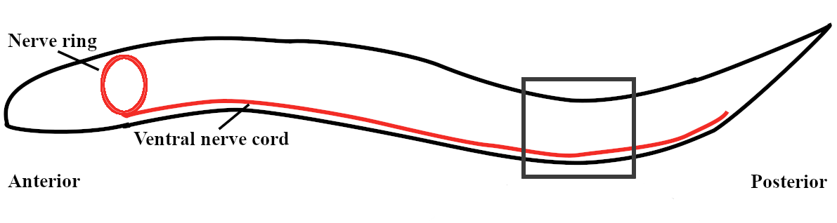
The central goal of neuroethology is to understand how an organism’s body and nervous system interact with its environment to produce behaviors such as locomotion. Model organisms have been used to study the complex interactions between the nervous system, body mechanics, and environmental dynamics in generating and coordinating locomotion [18, 25]. Some studies of locomotion in model organisms highlight feedforward control of locomotion, where the nervous system drives motor activity and sensory feedback plays only a modulatory role; these include legged locomotion in cockroaches and swimming in lamprey, crayfish, and leeches [8, 15, 18, 28, 37, 38, 39, 42, 46]. However, other systems such as stick insect locomotion are better understood as integrated neuromechanical systems because sensory feedback is essential to coordinating movements [4, 24, 34]. This sensory feedback is necessary for navigating more complex environments and can often lead to gait adaptation [1]. The nematode C. elegans is an ideal model organism for studying locomotion in an integrated neuromechanical setting because of its relatively simple and fully-described nervous system [44], limited stereotypical locomotive behavior [32], dependence on sensory feedback for forward locomotion [35, 43], and undulatory gait that adapts to different fluid environments [3, 13, 40].
C. elegans locomote forward using alternating dorsal and ventral body bends that propogate from anterior to posterior. The properties of this undulatory gait adapt to fluid environments of different viscosities: higher external fluid viscosities result in slower undulations of shorter wavelengths [3, 13, 40]. In water, C. elegans swim with a relatively long wavelength and relatively fast undulation frequency (roughly 1.5 bodylengths and 1.8 Hz) [13]. On agar, C. elegans crawl with a short wavelength and slow undulation frequency (0.65 bodylengths and 0.3 Hz) [13]. Previously, it was thought that these were two distinct gaits (swimming vs. crawling). However, recent experiments have shown that the wavelength and frequency of swimming in highly viscous fluids resemble crawling on agar surfaces [3, 13], and instead of a sharp swim/crawl transition, there is a smooth transition between the two gaits as the fluid viscosity of the environment is varied [3, 13, 40].
There are several hypotheses for how the undulatory gait is generated and coordinated [16]; however, it is generally agreed that proprioception plays a key role [5, 30, 43]. One hypothesis is that there is a central pattern-generating (CPG) neural unit in the head that initiates the propagation of the bending wave — higher fluid viscosities slow the propagation and shorten the wavelength [43]. Another hypothesis is that the ventral nerve cord consists of a network of neural modules that are capable of either (i) intrinsic neural oscillations [33] or (ii) neuromechanical oscillations (i.e., involving an entire feedback loop from neural to muscular to body mechanics and back through proprioception) [5, 6]. Recent experiments support the presence of multiple neural or neuromechanical oscillators [14] and the important role of proprioception in coordinating the oscillations [21].
Previous neuromechanical models consisting of a chain of neuromechanical oscillators (i.e., local oscillations driven by proprioceptive inputs) have been able to reproduce the undulatory waveform and gait adaptation [5, 12]. Boyle et al. [5] showed that a mechanistic neuromechanical model driven by proprioception could reproduce the continuous swim-crawl transition. Denham et al. [12] examined a similar neuromechanical model and through computational explorations showed how the mechanical properties and neural parameters affect gait adaptation in proprioceptively-driven control. However, the relative contributions to gait adaptation of each of the individual coupling modes (mechanical, gap-junctional, and proprioceptive coupling) are not well understood.
Here, we introduce a neuromechanical model of the C. elegans forward locomotion system that consists of a chain of neuromechanical oscillators coupled by gap-junctions and nearest-neighbor proprioception. We use our model to systematically analyze the role of body mechanics, gap-junctional coupling, and proprioceptive coupling in gait adaptation. The model captures the experimentally observed wavelength-trend of gait adaptation over a wide range of parameters, provided that the muscle response to input from the nervous system is faster than the body response to changes in force. We also find that sufficiently strong gap-junctional coupling is essential to achieving the long-wavelengths in our model. The modular structure of our model allows the use of the theory of weakly coupled oscillators to further dissect out the mechanisms underlying gait adaptation. Specifically, we assess the influence of each coupling modality (mechanical, gap-junctional, and proprioceptive). We find that proprioceptive coupling leads to a posteriorly-directed traveling wave with a characteristic wavelength. Gap-junctional coupling promotes synchronous activity (long wavelength), and mechanical coupling promotes a high spatial frequency (short wavelength). The wavelength of the undulatory waveform is set by the relative strengths of these three coupling forms. As the external fluid viscosity increases, the mechanical coupling strength increases and the wavelength decreases, resulting in the observed wavelength trend of gait adaptation.
2 Neuromechanical Model
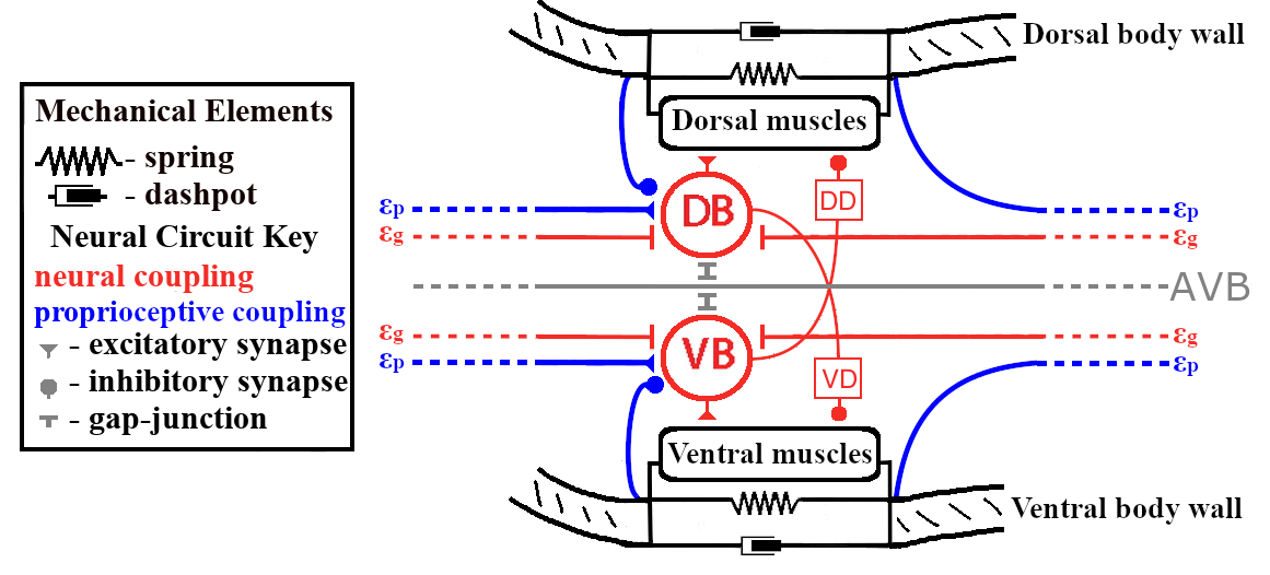
The neuromechanical model developed here describes the motor circuit, body-wall muscles, and the resulting body shapes of C. elegans. The body description is derived from a continuous centerline-approximation of an active viscoelastic beam, whereas the muscles and neural subcircuits are discrete in nature. The mechanical model is similar to that used in [13, 40, 43]. The model for the motor circuit uses the repeated motif of Haspel and O’Donovan [17]: 6 modules of roughly 12 motor neurons and 12 muscle cells, of these 12 repeated motor neurons roughly 6 (2 ventral B-class, 2 ventral D-class, 1 dorsal B-class, and 1 dorsal D-class neurons) are responsible for forward locomotion. In our model, we collapse the pair of VBs into a single compartment and the pair of VDs into a single compartment. We use a simplified version of Haspel and O’Donavan’s connectivity scheme [17], detailed in Section 2.1.3 and shown in Figure 1. Previous models present various simplified circuits [6, 5, 7, 12, 19, 31], and our model is most similar to [5], except that we omit the VD-to-VB inhibition. The model also includes proprioception: the B-class motor neurons respond to bending in the local and nearest anterior regions of the body [43, 48].
A schematic of our neuromechanical model is shown in Figure 1, which highlights the modular structure of the neural circuit, body-wall muscles, and the corresponding body region. Within each module, the motor subcircuit drives the body-wall muscles, which in turn apply contractile forces to bend the corresponding body region. The body mechanics then feed back into the neural circuit through proprioceptive feedback, which translates body-wall length changes into neural signals. This structure allows each module to function, in isolation, as a neuromechanical oscillator, and it suggests that the full body functions as a system of coupled neuromechanical oscillators.
2.1 Model Development
2.1.1 Body Mechanics
The nematode body is modeled as an active viscoelastic beam for small amplitude displacements submerged in a Newtonian fluid. C. elegans usually operates in a regime where inertia plays a minor role (i.e., low Re), thus the equation of motion is a balance of internal elastic forces, internal viscous forces, and a fluid drag force described by a local drag coefficient [13, 40, 45]:
| (1) |
where is the length-wise body coordinate, is time, is the displacement in the ventral-dorsal plane, is the curvature, and is the active moment that comes from internal muscle activity. The parameter is the bending modulus, is the effective internal viscosity, and the normal drag coefficient is proportional to the external fluid viscosity (, see Appendix B). The values for these parameters are given in Table 1, and a discussion of how they were selected is provided in Section 2.3.
We consider small amplitude undulations, so that the curvature is approximately the second spatial derivative of the displacements :
| (2) |
Taking two partial derivatives in of equation 1 and applying force-free, moment-free boundary conditions, the curvature of the body satisfies
| (3) | |||||
| (4) | |||||
| (5) | |||||
where is the head and is the tail ( is the body length). Note that in equations 3-5, a positive curvature represents a bend towards the dorsal side. The active moment comes from internal muscle activity, which will be defined below.
2.1.2 Muscles
The body is driven by six modules of roughly 6 ventral and 6 dorsal muscle cells, that apply contractile forces to either the dorsal or ventral side [17, 48]. These muscle modules split the body into six distinct regions of length . Each ventral/dorsal muscle group applies a contractile force as a function of its activity level . The ventral and dorsal () muscle activities in the module are given by
| (6) |
where is the timescale of muscle activation and is the input from the neural module (described below). The tension generated by the muscle is only contractile () and saturates at some peak force :
| (7) |
where define the scale and shift of the nonlinear threshold. In the module, the dorsal and ventral muscles apply contractile forces to opposite sides of the body, which induces a moment on the centerline from to :
| (8) |
The active moment as a function of the body coordinate is then given by
| (9) |
2.1.3 Neural Module
The motor neurons necessary for forward locomotion are the DB (dorsal B-class) and VB (ventral B-class) [17, 48], and the neurons DD (dorsal D-class) and VD (ventral D-class) have been predicted as necessary for swimming [5, 11]. Figure 1 shows the neural module used in our model. There are 11 VB, 13 VD, 7 DB, and 6 DD neurons in the ventral nerve cord, which corresponds to about 2 VB, 2 VD, 1 DB, and 1 DD neurons in each of the six modules in our model [17]. In each module, the pair of VB neurons are connected via gap-junctions and have similar inputs and outputs, so we model each pair of VB neurons as a single entity. We assume the same for each pair of VD neurons. The neural modules in our model are similar in structure to Boyle et al. [5], except that we omit the VD-to-VB inhibition. Each neural module is driven by constant input from the head interneuron AVB [17, 44, 48]. The D-class neurons are assumed to invert excitation from the B-class neurons into inhibition of the contralateral muscles. The B-class neurons are modeled as bistable, non-spiking elements, in line with recordings of similar motor neurons involved in head-turns [26]. The activities of the ventral and dorsal () B-class neurons in the neural module are given by
| (10) |
where
| (11) |
Here, is the timescale of neural activity, and is the offset from the constant “on” input from AVB. is proprioceptive feedback into the neuron, and is gap-junctional (electrical) coupling between neurons, both of which will be described below.
The D-class neurons are excited by the ipsilateral B-class neurons and inhibit the contralateral body-wall muscles. This effect is captured by direct inhibition of the muscles by the B-class neurons. We model the B-class neurons as exciting the ipsilateral muscles and inhibiting the contralateral muscles. The input from the neural module to the ventral/dorsal muscles is given by
| (12) |
2.1.4 Proprioceptive Feedback
To close the neuromechanical loop, the body segment curvatures feed back into the circuit via proprioceptive processes in the VB and DB neurons. There are two types of proprioception in this model: local (from the body region covered by the muscles of the module) and nonlocal (from neighboring anterior body regions).
Local proprioceptive feedback acts to reset the neural modules, i.e., switch between dorsal bend commands and ventral bend commands. Thus, local proprioception is modeled as an excitatory current to the ventral B-class neurons in response to positive average curvature over the local module of length , and an inhibitory current in response to negative average local curvature. The input to the dorsal B-class neurons is the same but with the polarities reversed. This feedback acts to relax the contracted muscles and contract the relaxed muscles.
Nonlocal proprioception promotes a wave of activity that propogates from anterior to posterior. The anatomical structures underlying proprioception are unknown [48], however, the evidence in Wen et al. [43] suggests that proprioceptive information affects the B-class motorneurons and is propagated posteriorly. To be consistent with this directionality, in our model positive nonlocal anterior segment curvature yields a weak inhibitory current to the ventral B-class neurons and a weak excitatory current to the dorsal B-class neurons. Negative nonlocal anterior segment curvature yields similar currents with the polarities reversed to each side. This same directionality was shown to produce locomotion in the earlier neuromechanical model of Izquierdo and Beer [19]. This is similar to the assumptions of Boyle et al. [5], but with the opposite directionality and sign of nonlocal proprioception.
The proprioceptive feedback to the ventral and dorsal B-class neurons in the neural module () of length is modeled by
| (13) | ||||
| (14) |
where is the strength of local proprioception, is the strength of nonlocal anterior proprioception, and for for notational simplicity.
2.1.5 Gap-Junctional Coupling
The B-class neurons are also connected via gap-junction synapses to neighboring B neurons of the same type (ventral/dorsal) [17, 44, 48]. The gap-junctions are modeled as symmetric ohmic resistors with constant conductance, so that the gap-junctional coupling to the ventral and dorsal () B-class neurons in the neural module are described by
| (15) |
where is the strength of gap-junction coupling and for notational simplicity.
2.2 Model Discretization for Numerical Simulation
To simulate the model described in Section 2.1, the body is discretized into six modules in correspondence with the six neuromuscular modules, so that there are six discrete body segment curvatures. The 4th-order difference operator is used to approximate the 4th spatial derivative with zero-force, zero-torque boundary conditions:
| (16) |
Discretizing equations 3-5 and using 8-9 yields a linear differential equation for the vector of body segment curvatures :
| (17) |
where is the identity matrix.
In this discretization, the neural and muscle activity dynamics of all the modules are given by
| (18) | ||||
| (19) | ||||
| (20) | ||||
| (21) |
where each vector entry (e.g., ) is the corresponding activity of the module. In equations 20 and 21, is the nonlocal proprioceptive connectivity matrix (equation 22), which comes from discretizing equation 13, and is the gap-junction connectivity matrix (equation 23), which comes from discretizing equation 15:
| (22) |
| (23) |
2.3 Parameter Discussion
Some parameters in the model are well-constrained by experimental data, while others are not. Quantities that are directly measurable include the body length mm, average body radius m, cuticle width m, and wavelength and frequency in fluids of various viscosities . The timescales in the system are less certain. The range 50-200 ms is used for the muscle activation timescale , which is the range of measurements of peak muscle force generation time in Milligan et al. (1997) [27]. As with previous models [5, 12, 19], the neural activity is chosen to be the fastest process in the model, but while Boyle et al. [5] considered the B-neurons as instantaneous switches, here the neural activity timescale is set at ms.
The internal viscosity and Young’s modulus have been estimated across several orders of magnitude [2, 13, 40], so caution is exercised in using one set of parameters from one source over another. Of more importance in the model is the mechanical timescale
| (24) |
which is the timescale of relaxation in an inviscid fluid. In equation 24, is the bending modulus, which is derived from the Young’s modulus and the geometry of the cuticle in Appendix B following previous modeling procedures [10, 40]. In Appendix B, we also compare the range of mechanical parameters used here with previous models. Given the range of mechanical parameters reported in the literature, the mechanical timescale could be as small as ms or as large as s. The role of this timescale is explored in Section 3.2.
The electrophysiological details of the internal neural circuit are largely unknown, thus all the feedback and coupling strengths , the parameters of the nonlinear functions and are not well constrained. The feedback strengths , and parameters of the nonlinear functions () and () were chosen so that the neuromechanical oscillator robustly gives the correct frequency () in a low-viscosity environment. The values for the coupling parameters and , on the other hand, are explored in the next section.
| Parameter | Name | Range of values | References |
|---|---|---|---|
| Body length | 1 mm | [44] | |
| Average body radius | 40 m | [9] | |
| Cuticle width | 0.5 m | [9] | |
| E | Young’s modulus | kPa - kPa | [2, 13, 40] |
| Second moment of area of cuticle | [9] | ||
| Bending modulus | N(mm)2 | [2, 13, 40] | |
| Body viscosity | N(mm)2s | [2, 13, 40] | |
| Fluid viscosity | mPas | [13] | |
| Normal drag coefficient | [9, 13] | ||
| Mechanical timescale | 1 ms - 5 s | [2, 13, 40] | |
| Muscle activation timescale | 50-200 ms | [27] |
3 Model Results
C. elegans locomote forward using alternating dorsal and ventral body bends that propogate in the form of a traveling wave from anterior to posterior. The spatial wavelength of this traveling wave changes in response to changes in the fluid viscosity [3, 13, 40]. In this section, we show that our model captures this gait adaptation for a wide range of mechanical and neural parameters, provided that the muscle response to input from the nervous system is faster than the body response to changes in internal and external forces. We also show that sufficiently strong gap-junctional coupling is essential to achieving the long-wavelengths in our model.
3.1 Model Captures Gait Adaptation
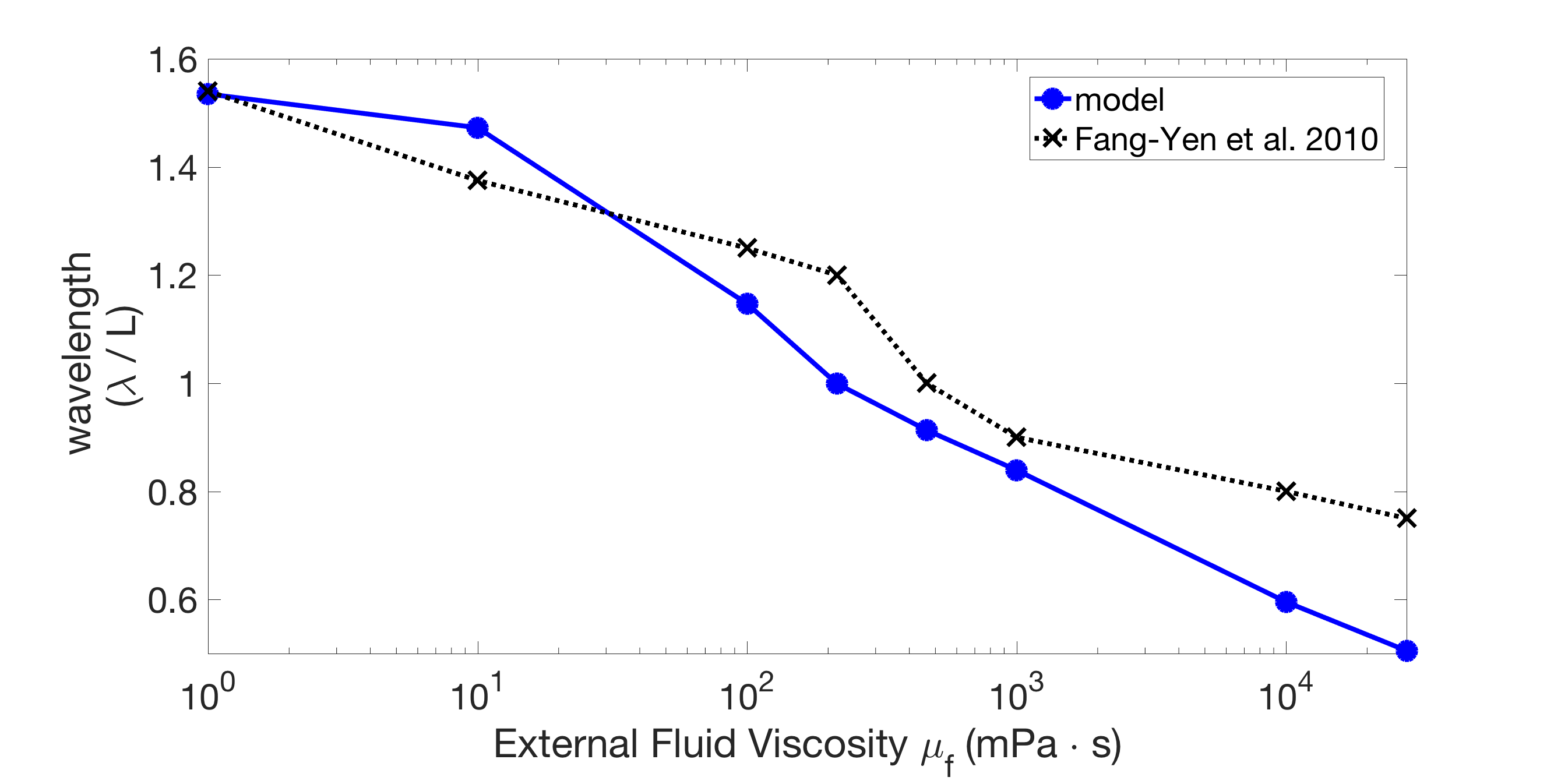
We fit the model to match the wavelength and frequency in water, and then ran it in different fluid environments. Our model captures the quantitative effect of external fluid viscosity on the body wavelength seen in experiments and previous models. Figure 2 shows an example of the wavelength trend of the model for fixed body parameters ms, ms (the wavelengths were computed from the model output as described in Appendix A). Figure 2 also shows that the model wavelengths are in close quantitative agreement with the experimentally-measured wavelengths of Fang-Yen et al. [13]. In water ( mPas) the wavelength is roughly 1.5 bodylengths, and increasing the fluid viscosity smoothly reduces the wavelength down to roughly 0.75 bodylengths in the most viscous case ( mPas). This wavelength trend is similar to what has been observed in other experiments [3, 40], and in Section 3.2, we show that our model captures this trend robustly over a wide range of parameters.
The undulation frequency also changes in response to changes in the fluid viscosity [3, 13, 40]. In Fang-Yen et al. [13], the frequency decreases from 1.7 Hz to 0.30 Hz as fluid viscosity increases from 1 mPa s to mPa s. Our model also exhibits a decrease in frequency as fluid viscosity increases, but not of the same magnitude (1.7 Hz - 1.6 Hz). Discussion of this discrepancy is given in Section 5.
3.2 Parameter Study Highlights Importance of Timescale Ordering in Capturing Gait Adaptation
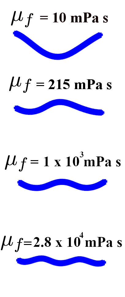
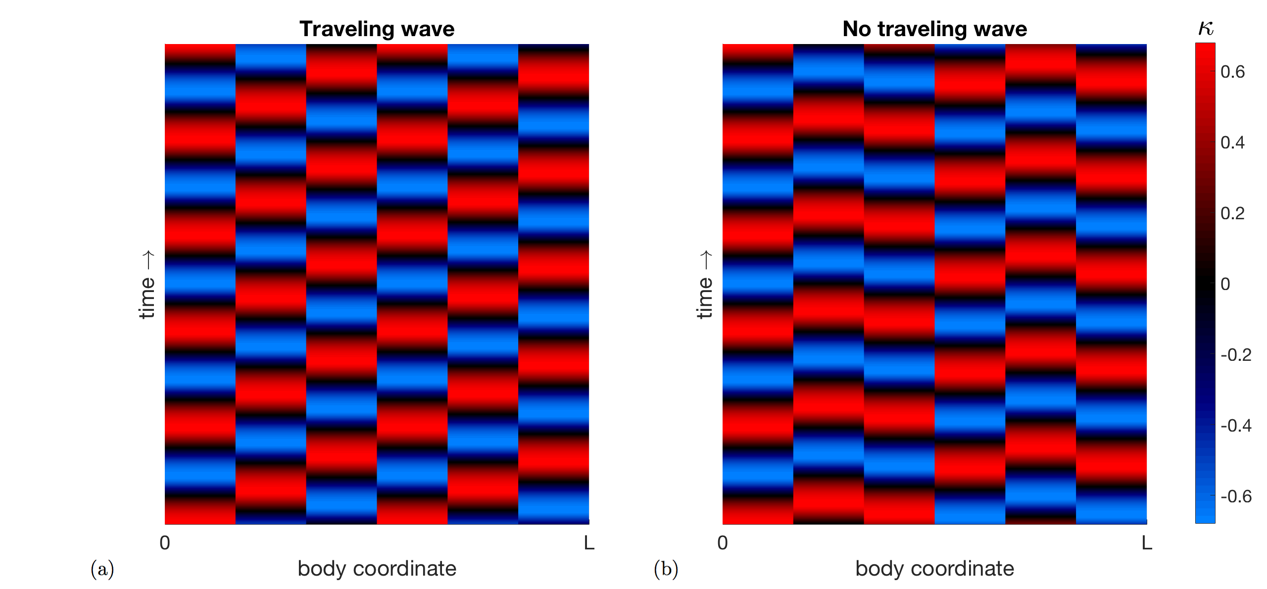
We performed a parameter study to show that the model robustly captures gait adaptation as the fluid viscosity is varied. The mechanical parameters , , the proprioceptive coupling strength , and the muscle timescale were varied, while the other parameters of the model were held fixed, including the gap-junctional coupling strength . (For more extensive parameter explorations, see [22].) For some parameter regimes, the body deformations were traveling waves for all fluid viscosities , but this was not the case for other parameter regimes. Figure 3 shows kymographs of the body curvature that demonstrate two typical cases exhibited by the model.
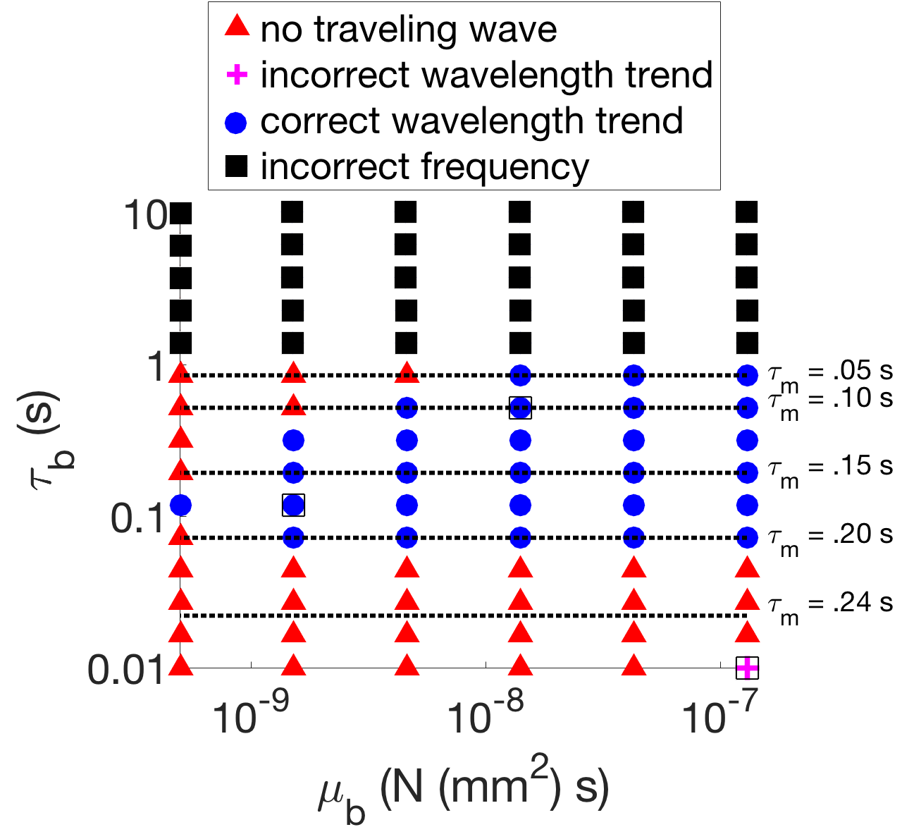
The model parameters , , and were systematically varied to characterize the model behavior. For a given body timescale and body viscosity , the muscle activity timescale was selected in the range 50-250 ms to match the undulation frequency (1.7 Hz) in water ( mPa s) within 1%. Next, the proprioceptive coupling strength was selected to match the wavelength (1.5 bodylengths) in water within 1%. We are able to separate these effects and perform these one-parameter searches due to the weakly coupled nature of our model. The model was then run in different fluid viscosity environments and the emergent coordination trend is reported in Figure 4. The model behavior was classified exclusively as either: (1) not a traveling wave for all fluid environments, (2) incorrect wavelength trend, (3) qualitatively correct wavelength trend, or (4) incorrect frequency in water.
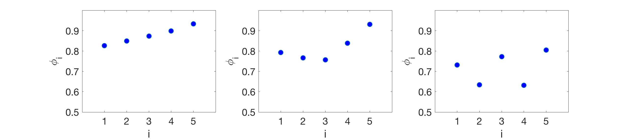
There is no traveling wave (red triangles) if, for any viscosity , the difference between the minimum and maximum pairwise-phase difference is greater than or equal to 0.5, because this indicates that there is no consistent directionality to the phase differences in the body. A range of observed wavelength trends in various parameter regimes (the boxed markers in Figure 4) are illustrated in Figure 5. Figure 5(a) and (b) show examples of the qualitatively correct wavelength trend (blue circles), while (c) shows the the incorrect trend, which was only obtained at a single parameter combination. The wavelength trend is incorrect because the wavelengths increased dramatically as the fluid viscosity increased, as opposed to generally decreasing.
(a)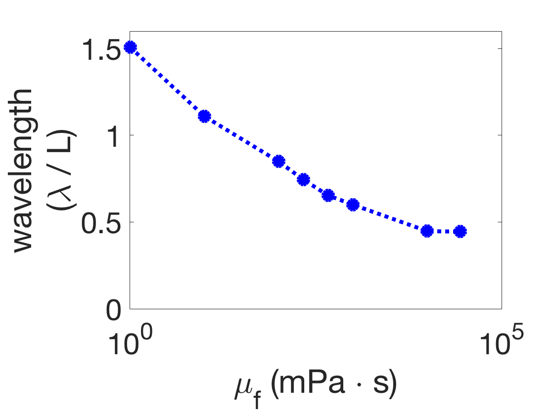 (b)
(b)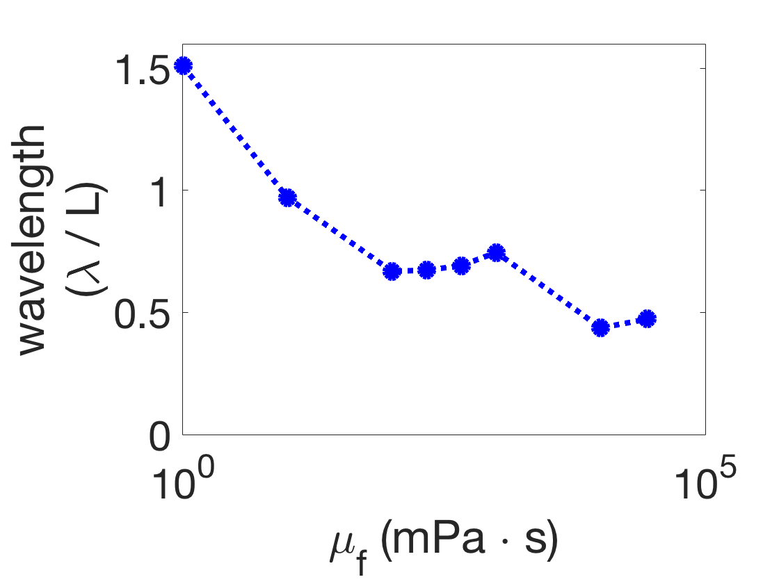 (c)
(c)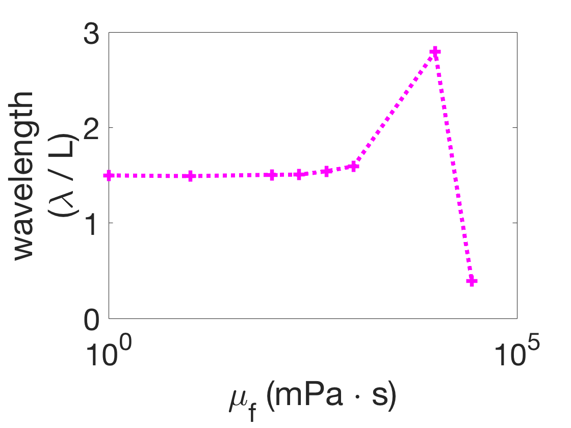
A few key observations can be made from Figure 4. First, if the mechanical timescale is too large, then the frequency in water cannot be obtained (see the black squares in Figure 4). Second, if the mechanical timescale is too small, then there will not be a traveling wave for all fluid viscosities . This suggests that while the body stiffness and body viscosity have been estimated across several orders of magnitude in various experiments and models, the effective mechanical body timescale lies within the relatively narrow range s.
In order to match the frequency, the muscle timescale must be inversely related to . When the body timescale is increased, the muscle timescale must decrease to compensate. The frequency in water cannot be obtained for too large since it would require decreasing the muscle activity timescale below physiological limits. Similarly, when the body timescale is decreased, the muscle timescale must be increased to compensate for the frequency. For too small, there is not a traveling wave for all fluid viscosities ; this occurs soon after . This suggests that the relative ordering of the timescales is key to the coordination. Generally, the mechanical timescale must be the largest, the muscle activity timescale intermediate, and the neural timescale the shortest. The mechanism by which this timescale ordering affects coordination is explained in Section 4.3.
Remarkably, whenever there is a traveling wave in this systematic parameter search, it almost always has the qualitatively correct wavelength trend. This wavelength trend is consistent with gait adaptation across several orders of magnitude of the mechanical parameters.
3.3 Gap-Junctions are Necessary for Long Wavelengths in the Model
To determine the role of gap-junctions in our neuromechanical model, we investigate how changing the gap-junctional coupling strength affects the wavelength trend and overall coordination. Other models have achieved accurate wavelength adaptation without gap-junctional coupling, albeit with proprioceptive ranges longer than nearest-neighbor [5, 12], so we assess the degree to which gap-junctional coupling is necessary in our model. We find that in our model, sufficiently strong gap-junctional coupling is necessary to obtain the long wavelengths in low-viscosity environments (e.g. water).
We vary the gap-junctional coupling strength in our model over several orders of magnitude ( and ). We fix the parameters s, s, and Ns and find the proprioceptive coupling strength to match the wavelength in water (approximately 1.5 bodylengths). Figure 6(a) shows the resulting wavelength trend of the model for different gap-junctional coupling strengths . For sufficiently strong gap-junctional coupling strengths (), the wavelength in water was matched and the full range of wavelength adaptation was found (circle-markers in Figure 6(a)). For weaker gap-junctional coupling strengths (), the wavelength in water was not matched (plus-markers, Figure 6(a)). We further show that the model with weak gap-junctional coupling strength () cannot match the wavelength in water for any proprioceptive coupling strength. Figure 6(b) shows the model wavelengths in water as a function of proprioceptive coupling strength for different gap-junctional coupling strengths and reiterates that the model cannot match the long wavelength without sufficiently strong gap-junctional coupling. Our neuromechanical model thus relies on gap-junctional coupling between neural modules to achieve the long wavelengths in low-viscosity environments.
(a)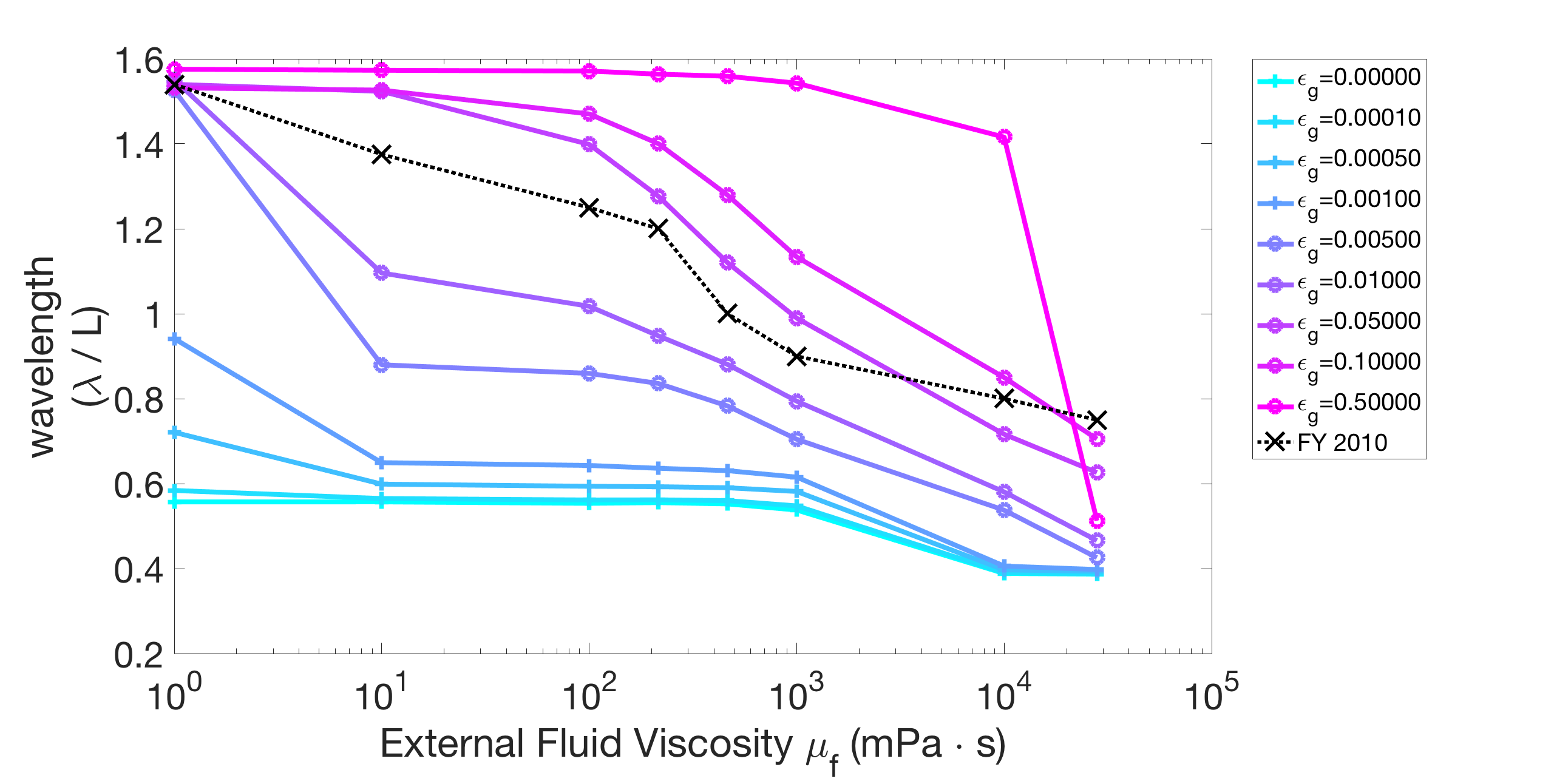 (b)
(b)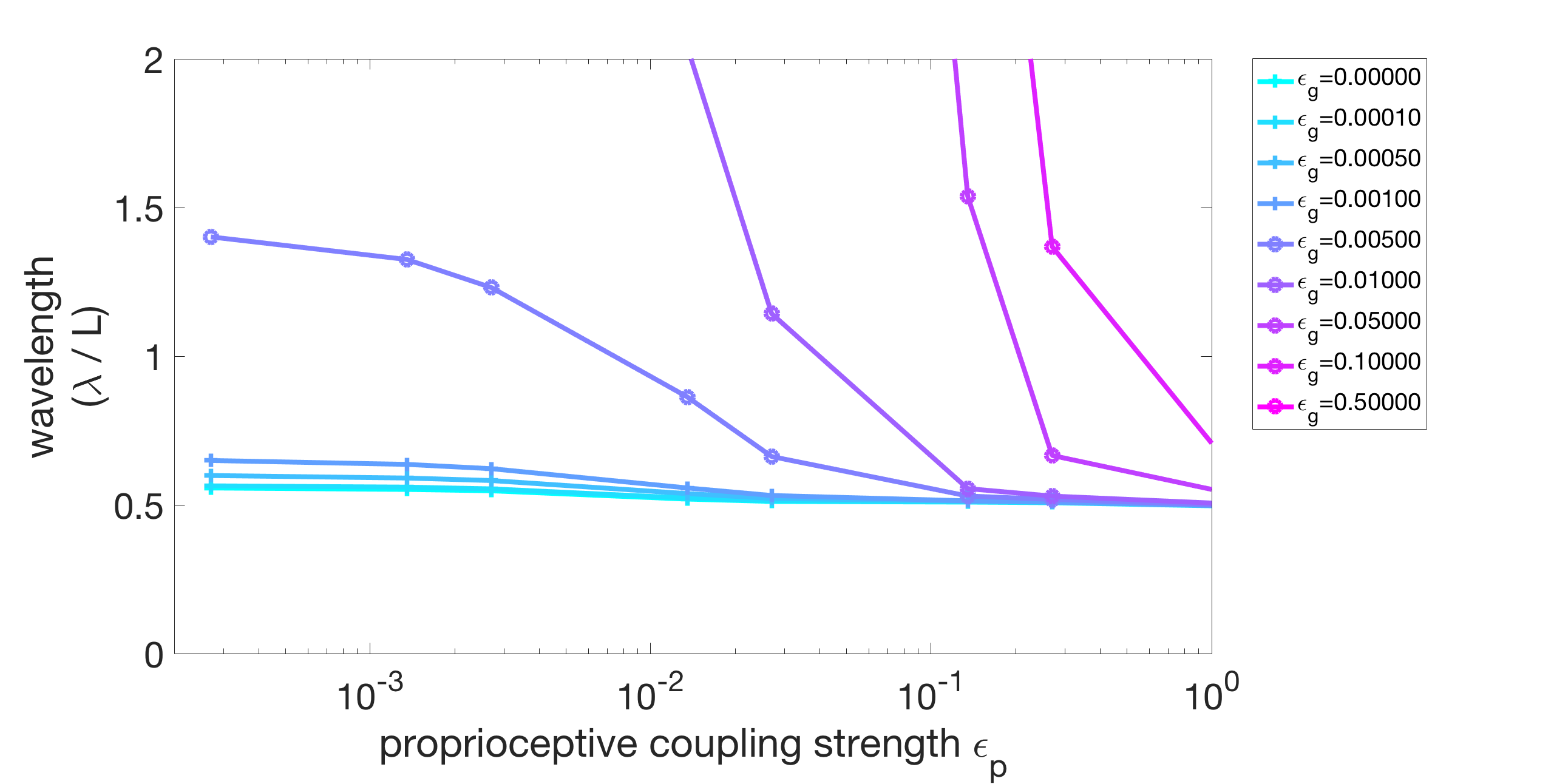
4 The Neuromechanical Model as a Network of Coupled Oscillators: Insight Into Mechanisms Underlying Gait Adaptation
The neuromechanical model is able to robustly capture the quantitative trend of gait adaptation across a wide range of parameters. In this section, the modular structure of the model will be exploited to uncover the fundamental mechanisms underlying gait adaptation. In Section 4.1, we show that the isolated neuromechanical modules are oscillators. (Note that from the standard theory of weakly coupled oscillators point of view the modules would be considered “intrinsic oscillators”, whereas from a neurolocomotion perspective, the modules are “extrinsic oscillators”, i.e., local proprioceptive feedback is required to generate the oscillations.) These modules form a network of coupled oscillators with three forms of coupling: mechanical (through the body and external fluid), proprioceptive, and gap-junctional. Furthermore, this coupling is relatively weak, and thus the theory of weakly coupled oscillators [23, 36] can be applied to identify the coordinating effects of each coupling modality. We demonstrate that the competition between mechanical coupling and neural coupling provides an explicit mechanism for gait adaptation.
4.1 Isolated Neuromechanical Modules are Oscillators
A single, isolated neuromechanical module is defined as a neural subcircuit, the corresponding muscles and body section, and local proprioceptive feedback (without coupling through the body or neural circuitry). The dynamics for this isolated module are governed by
| (25) | ||||
| (26) | ||||
| (27) | ||||
| (28) | ||||
| (29) |
Note that this is the model described in Section 2, omitting the intermodular coupling. The isolated modules exhibit robust oscillations over a wide range of parameters, and a single period of the module is shown for each state-variable in Figure 7(a). Thus, the neuromechanical modules are oscillators, wherein each B-class neuron promotes either a dorsal or ventral bend and the local proprioceptive feedback acts to switch the bistable B neurons from one state to the other. The basic cycle of the oscillator is as follows: when activated, the ventral B-class neuron () excites the ventral muscles which build up activity () to induce a ventral bend (negative ); when the curvature is sufficiently large, the local proprioceptive feedback deactivates the ventral B-class neuron and activates the dorsal B-class neuron, and the cycle continues towards a dorsal bend.
The system of six identical, uncoupled neuromechanical oscillators is described by
| (30) |
where
| (31) |
and is given by equations 25-29. The oscillations correspond to a -periodic limit cycle in -state-space. This limit cycle can be parametrized by phase
| (32) |
with the initial phase . As increases at a constant rate , traces out the limit cycle through state-space and the state of each oscillator on the limit cycle is given by
| (33) |
where the only distinguishing feature between the oscillators is their unique phase . Figure 7(a) shows the components of .
(a)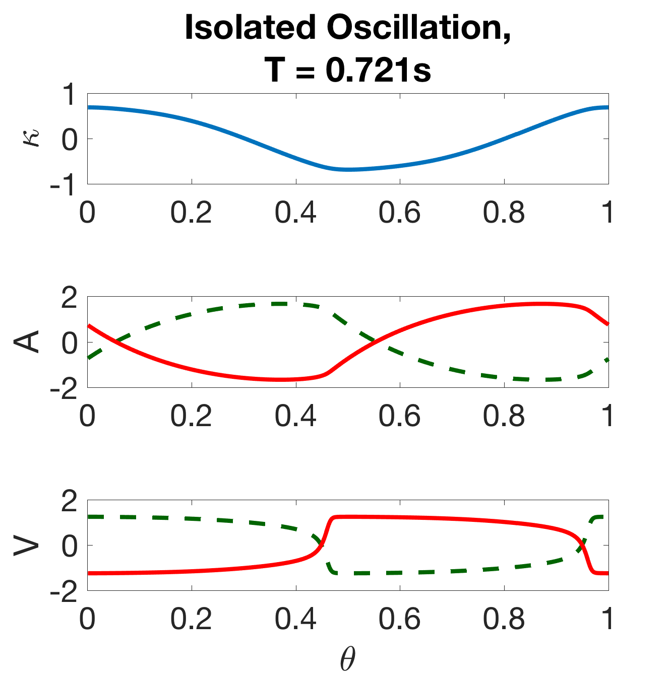 (b)
(b)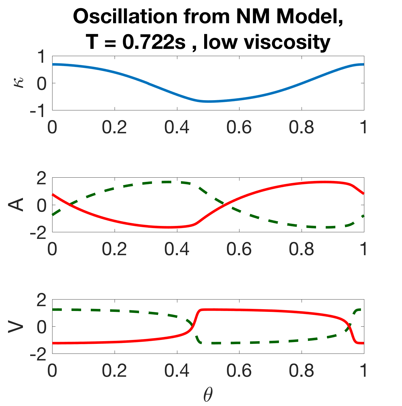 (c)
(c)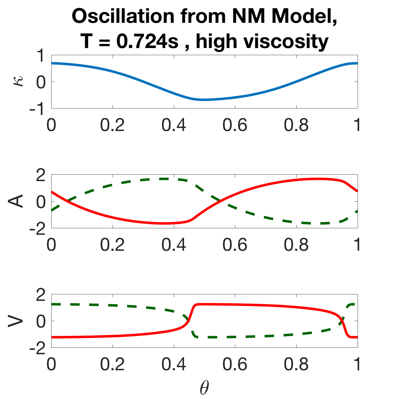
4.2 Network of Coupled Oscillators
Rearranging equations 17-23, the neuromechanical model can be written as a network of coupled oscillators:
| (34) |
where describes the coupling dynamics from all the modules to the module through gap-junctions, nonlocal proprioception, and body mechanics:
| (35) |
The parameter is the effective mechanical coupling strength.
The oscillations of the isolated module (equations 25-29) are indistinguishable (on the scale of Figure 7) from the oscillations of a module within the fully-coupled network (equations 17-21) at both low and high external fluid viscosity . That is, the dynamics of the coupled module never deviate substantially from the limit cycle of the uncoupled module. This indicates that the intrinsic dynamics of the module dominate over the influence of coupling on any given cycle, which implies that the coupling is “weak”. However, small changes in the phase of a module due to coupling can accumulate over many cycles to significantly influence the phase differences between the modules.
Because the coupling is weak (as defined above), the theory of weakly coupled oscillators can be applied (see [36] for details). The coupling only alters the phase of the oscillators on their respective limit cycles and the effect on amplitude is negligible, therefore the phase completely describes the state of a neuromechanical module. Equation 34 can be reduced to the so-called phase equations, a set of differential equations describing the evolution of the phases of each oscillator:
| (36) |
where is the phase of the oscillator, is the intrinsic frequency, and are the interaction functions that describe the change in frequency (resulting from either mechanical, proprioceptive, or gap-junction coupling) as a function of the phase difference of a given pair of oscillators:
| (37) | ||||
| (38) | ||||
| (39) |
Here, , , are the periodic phase response functions to perturbations in the corresponding state variable.
The coupling modalities define the structure of the interaction functions, through the state variables that are coupled, as well as the coupling topology (the connectivity matrices , , and in equation 36). Note that there is a separate H-function for each of the three coupling modalities and these three coupling modalities add linearly to produce the full interaction of the modules. Therefore, the relative contributions of the various coupling types can be analyzed independently through varying the different coupling strengths: fluid viscosity (through ) for mechanical, for proprioceptive, and for gap-junctional.
4.3 Two Oscillator Analysis Explains the Coordination Mechanism
Analyzing a pair of two coupled oscillators gives considerable insight into the coordination that each coupling modality produces separately and the mechanisms of coordination. With only two oscillators, the phase model reduces to
| (40) | ||||
| (41) |
In the two oscillator case, the matrix is symmetric, so . By defining
| (42) |
and subtracting equation 40 from equation 41, the dynamics of the two oscillator system can be described by a single differential equation for the phase difference between the two oscillators:
| (43) |
where , , and are the pair-wise interaction functions, or G-functions of the pair. The stable phase-locked state of the system is given by .
4.3.1 Each Coupling Modality Promotes a Different Coordination Outcome
Figure 8 shows the G-functions and corresponding phase-locked states of the different coupling modalities. For mechanical coupling alone, i.e., , the stable phase-locked state is anti-phase (), since and (Figure 8(a)). Similarly, for proprioceptive coupling alone, the stable state is an intermediate phase-difference (, Figure 8(b)), so the first oscillator leads the second (front-to-back). For gap-junctional coupling alone, the stable state is synchrony (, Figure 8(c)).
The coordination outcome with all three coupling mechanisms present corresponds to the zero of the G-function (equation 43), which is a weighted sum of the three individual G-functions. Thus, coordination can be examined in the context of this weighted sum as the three coupling strengths are varied: external fluid viscosity for mechanical coupling, proprioceptive coupling strength , and gap-junction coupling strength .
(a)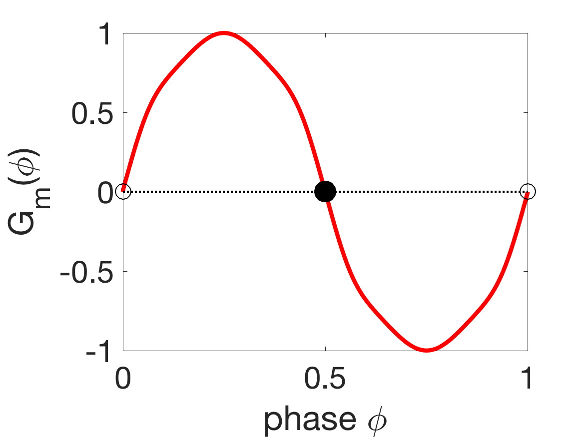 (b)
(b)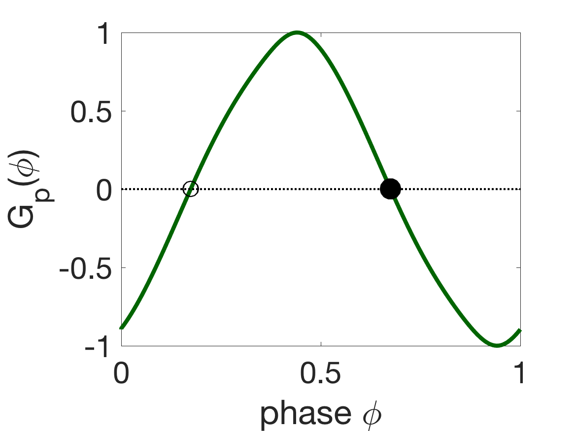 (c)
(c)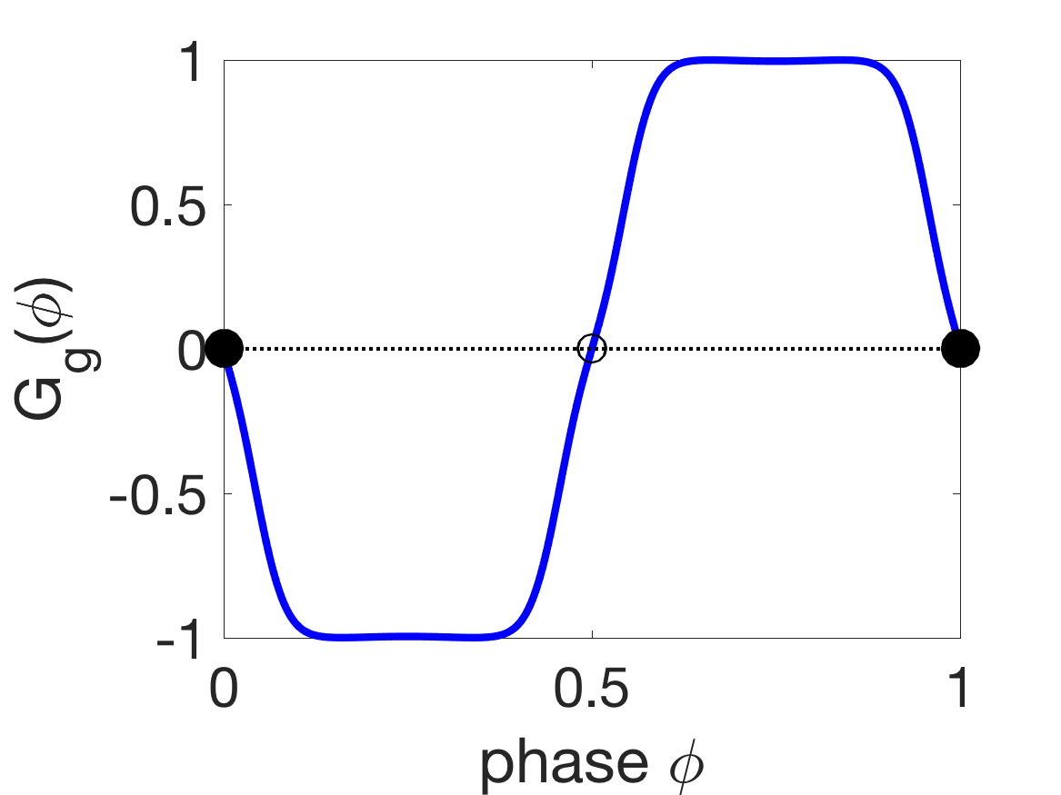
4.3.2 Neural Coupling Sets the Low-Viscosity Wavelength
(a)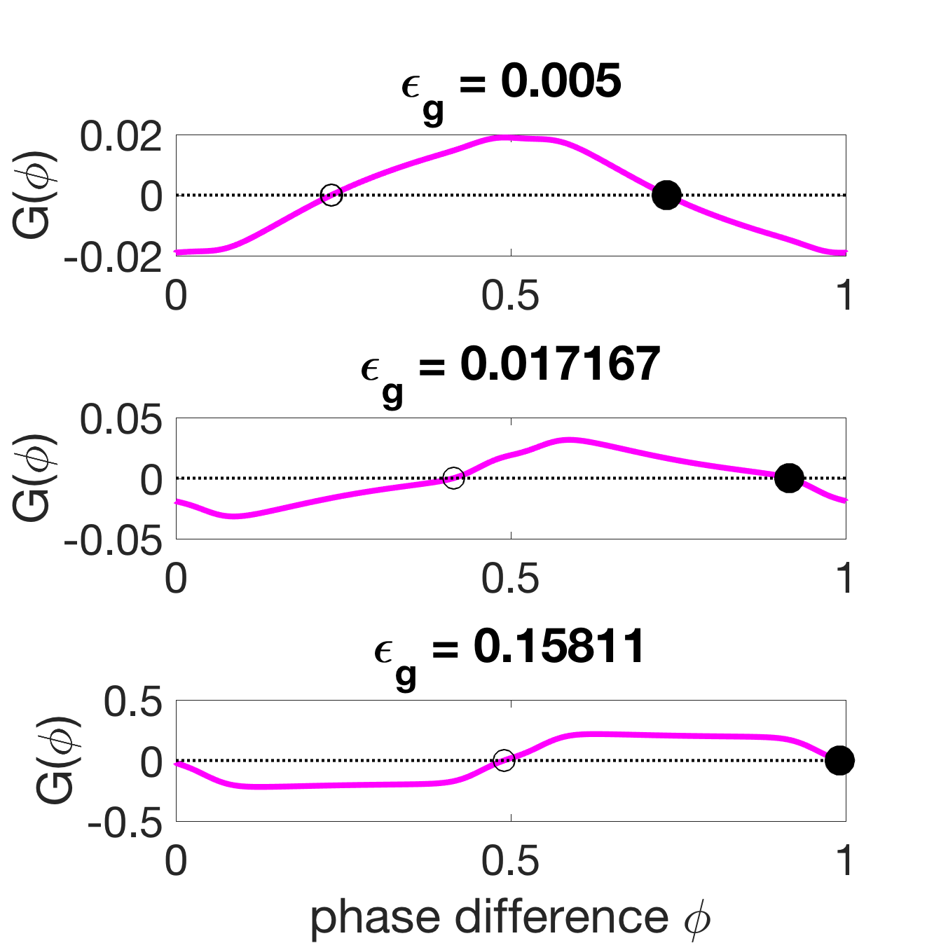 (b)
(b)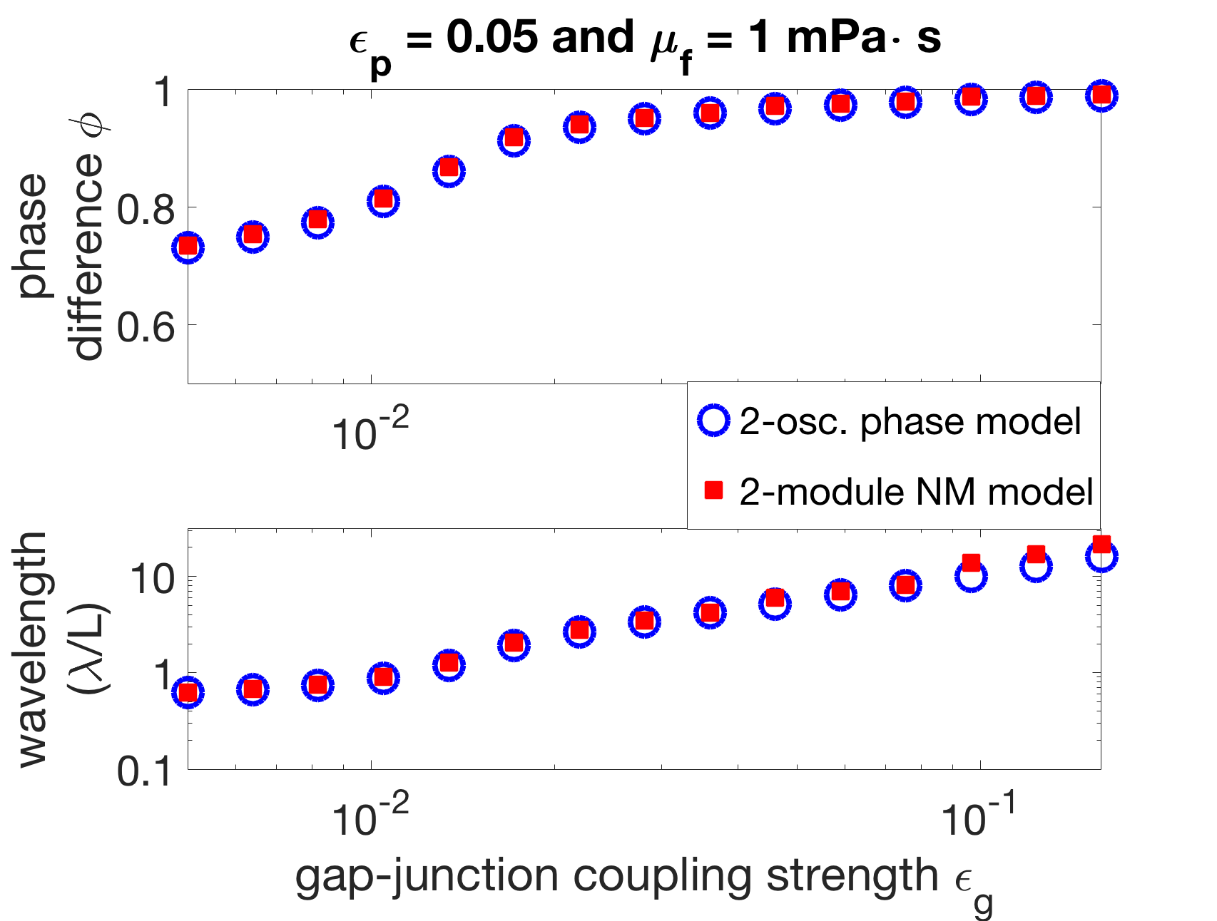
The stable phase difference of the pair of the neuromechanical oscillators can be used to define a wavelength in the full body (for details see Appendix A):
| (44) |
In the low external fluid viscosity case ( mPas), setting as in Section 3.2 provides a good approximation of the experimentally observed wavelength for the mechanical parameters N (mm)2, N (mm)2 s. For these parameters, the relative sizes of the G-functions in equation 43 are
| (45) | ||||
| (46) | ||||
| (47) |
Thus, at low viscosity, mechanical coupling is almost negligible compared to neural coupling, so the coordination is determined by proprioceptive and gap-junctional coupling.
How the wavelength is set in this low-viscosity case can be examined by varying the neural coupling strengths. Figure 9(a) shows that as the gap-junctional coupling strength is increased relative to the proprioceptive coupling strength, the phase-locked states move from close to the zeros of towards the zeros of . Figure 9(b) shows that when proprioceptive coupling dominates, the stable phase-locked state corresponds to a phase difference of roughly and corresponds to a wavelength of 0.75 bodylengths according to equation 44. When gap-junctional coupling dominates, the stable phase-locked state is close to synchrony , which corresponds to an infinite wavelength in the full body if this phase difference was constant. In this gap-junction-dominated case, each pair is in perfect synchrony and the body exhibits a standing wave.
To assess the predictive power of the two-oscillator phase model, a simulation of the neuromechanical model with only two modules was performed alongside the phase model. Figure 9(b) shows that the two-oscillator phase model is quantitatively accurate when compared to the phase differences and wavelengths derived from this two-module simulation. Thus, neural coupling sets the low-viscosity wavelength in the two-module neuromechanical model as well.
4.3.3 Competition Between Mechanical and Neural Coupling Provides a Mechanism for Gait Adaptation
(a)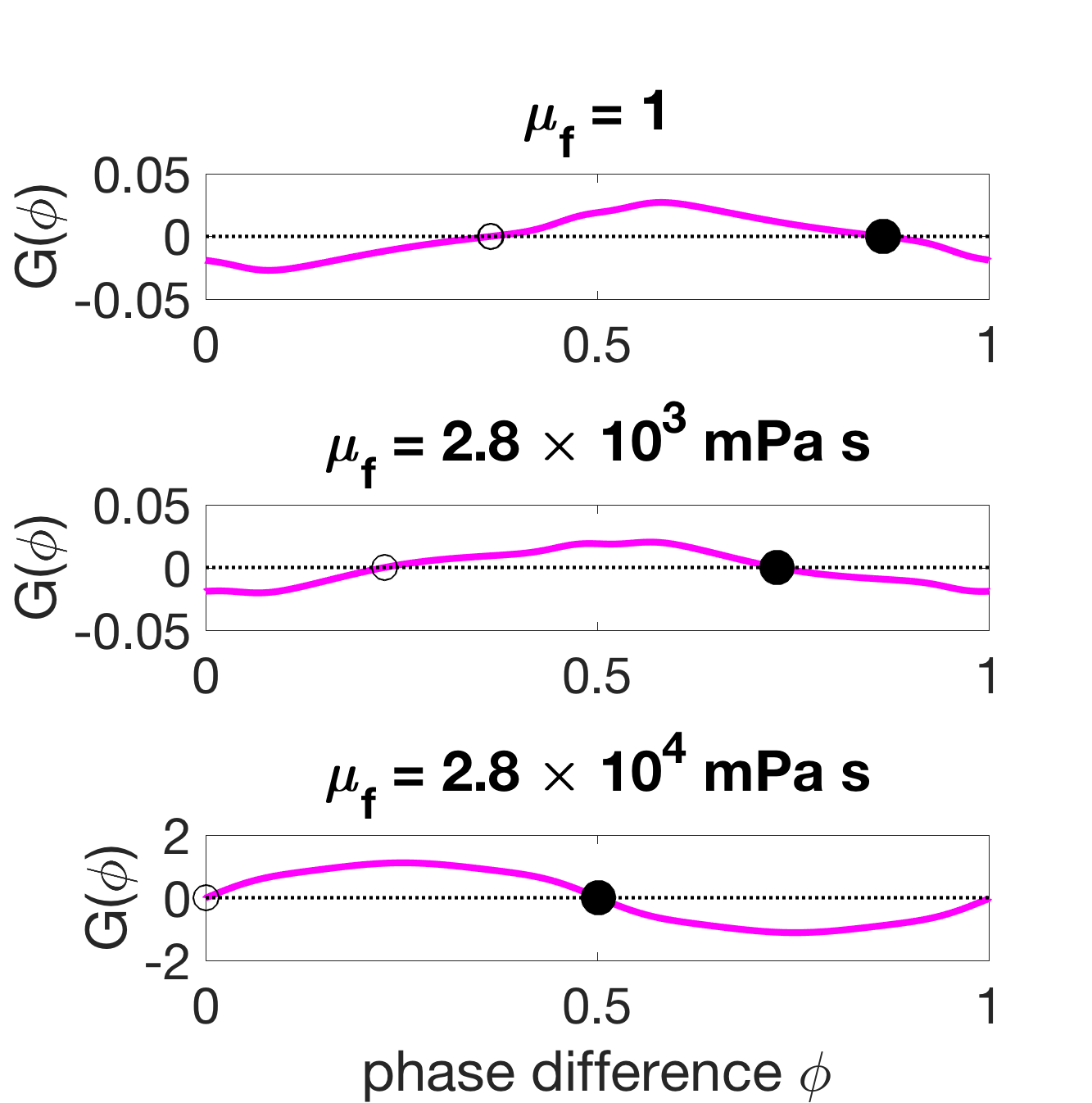 (b)
(b)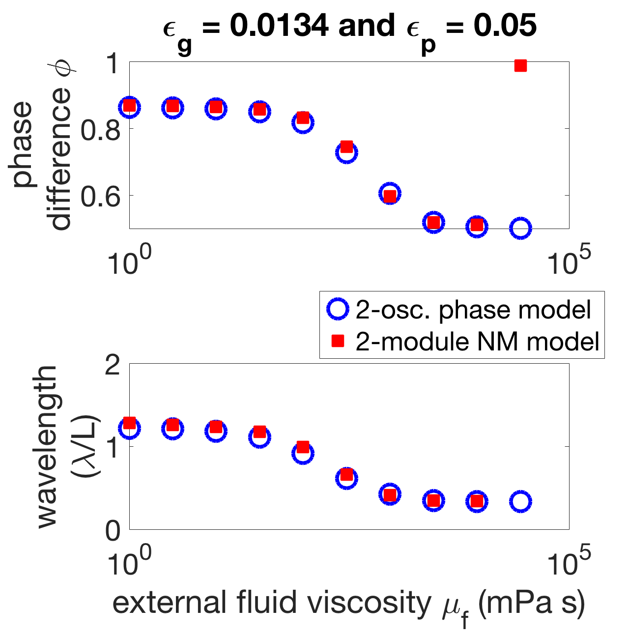
To examine the effect of mechanical coupling in the two-oscillator phase model, the neural coupling parameters are fixed to and so that the wavelength in the low-viscosity case is roughly 1.5 bodylengths. The strength of mechanical coupling is increased in equation 43 by increasing the external fluid viscosity . Figure 10(a) shows that as the strength of mechanical coupling is increased, the phase-locked states move from close to the zeros set by towards the zeros of . Figure 10(b) shows how the stable phase-locked state changes as a function of the mechanical coupling strength . When neural coupling dominates, the stable phase-locked state is a phase difference of roughly , and when mechanical coupling dominates, the stable phase-locked state is antiphase . Similarly, Figure 10(b) shows that when neural coupling dominates the resulting wavelength (according to equation 44) is roughly 1.5 bodylengths, and when mechanical coupling dominates the wavelength is roughly 0.45 bodylengths.
This analysis shows that gait adaptation is a result of competition between mechanical and neural coupling. The decrease in wavelength as external viscosity increases is explained by the increased strength in mechanical coupling and its associated coordination outcome, antiphase. The two-oscillator phase model is quantitatively accurate when compared to phase differences derived from the neuromechanical model with two modules, as shown in Figure 10(b). Thus, this suggests that the mechanism underlying the behavior in the two-module neuromechanical model is the same as the mechanism of the phase model outlined here. However, note that the phase difference at the highest fluid viscosity ( mPa s) is different between the two-oscillator phase model and the full two-module neuromechanical model. This indicates the limit of weak coupling, as the phase reduction is not able to capture the transition to synchrony seen in the two-module neuromechanical model. However, weak coupling holds in the two-oscillator case for the rest of the viscosities considered. Furthermore, this transition to synchrony is not seen in the six-module neuromechanical model.
4.3.4 Phase Reduction Gives Insight into Timescale Ordering
The phase reduction also explains why generally must be larger than in order to obtain the correct coordination trend (as described in Section 3.2). The results in the previous subsection indicate that it is important for mechanical coupling to promote antiphase in order to get the correct wavelength trend as external viscosity is increased. Figure 11(a) shows that, when is sufficiently larger than , the stable zero of is 0.5, i.e., the stable phase-locked state is antiphase. However, when is sufficiently smaller than , the stable zero of is 0, i.e., the G-function is flipped and mechanical coupling promotes synchrony. In this case, the wavelength trend as external viscosity is increased is incorrect, since increasing the mechanical coupling strength would pull the oscillators towards synchrony, lengthening the wavelength instead of shortening it.
The shift in the stabilities of the phase-locked states from antiphase to synchrony is somewhat complicated, as Figure 11(c) shows that can yield tristable phase-locked states. A series of paired saddle-node bifurcations and paired super- and sub-critical pitchfork bifurcations (Figure 11D), marks the transition from stable antiphase to tristability to stable synchrony as moves below . The change in the stability of the antiphase state promoted by mechanical coupling is the cause of the rapid change in coordination in Figure 4 as becomes sufficiently smaller than .
(a)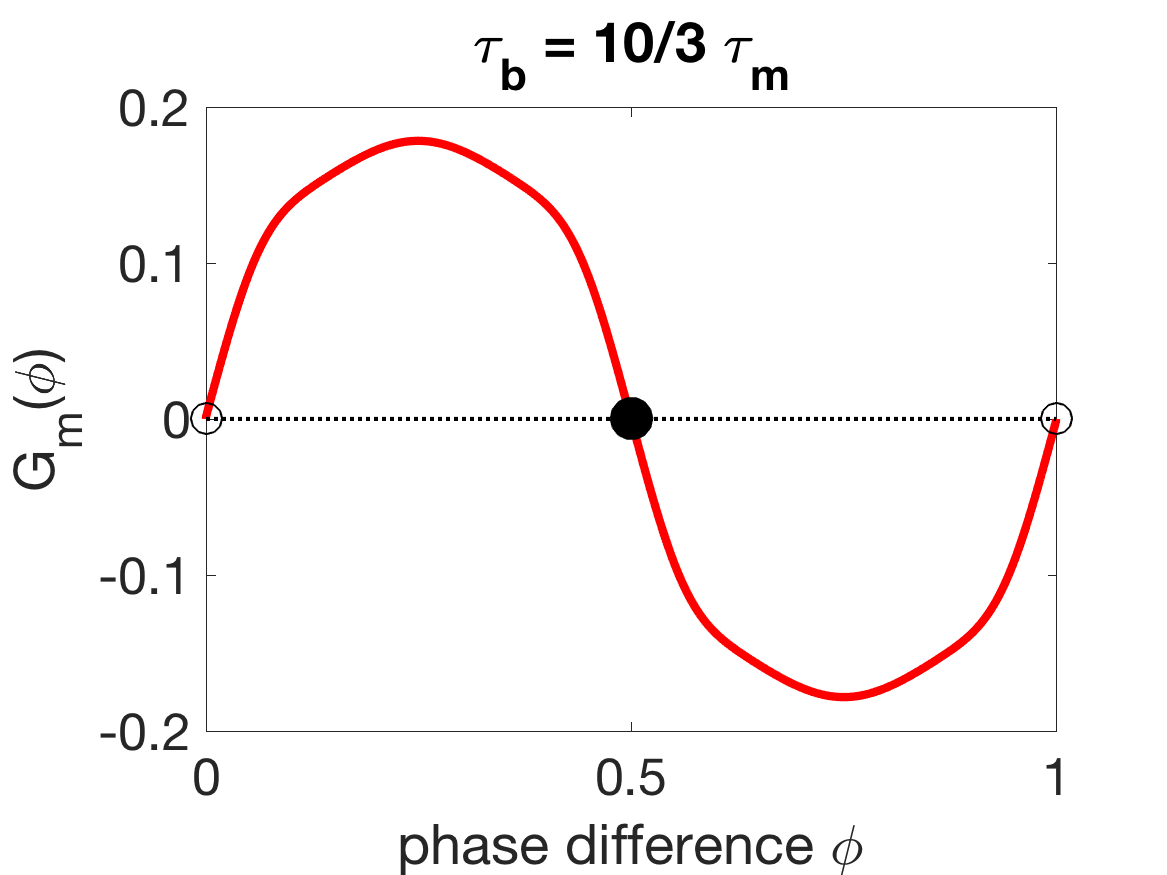 (b)
(b)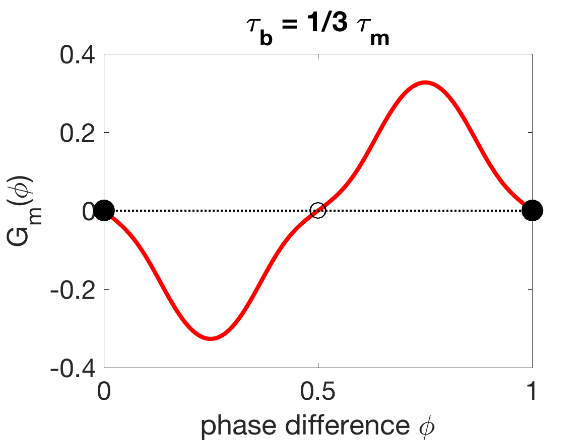
(c)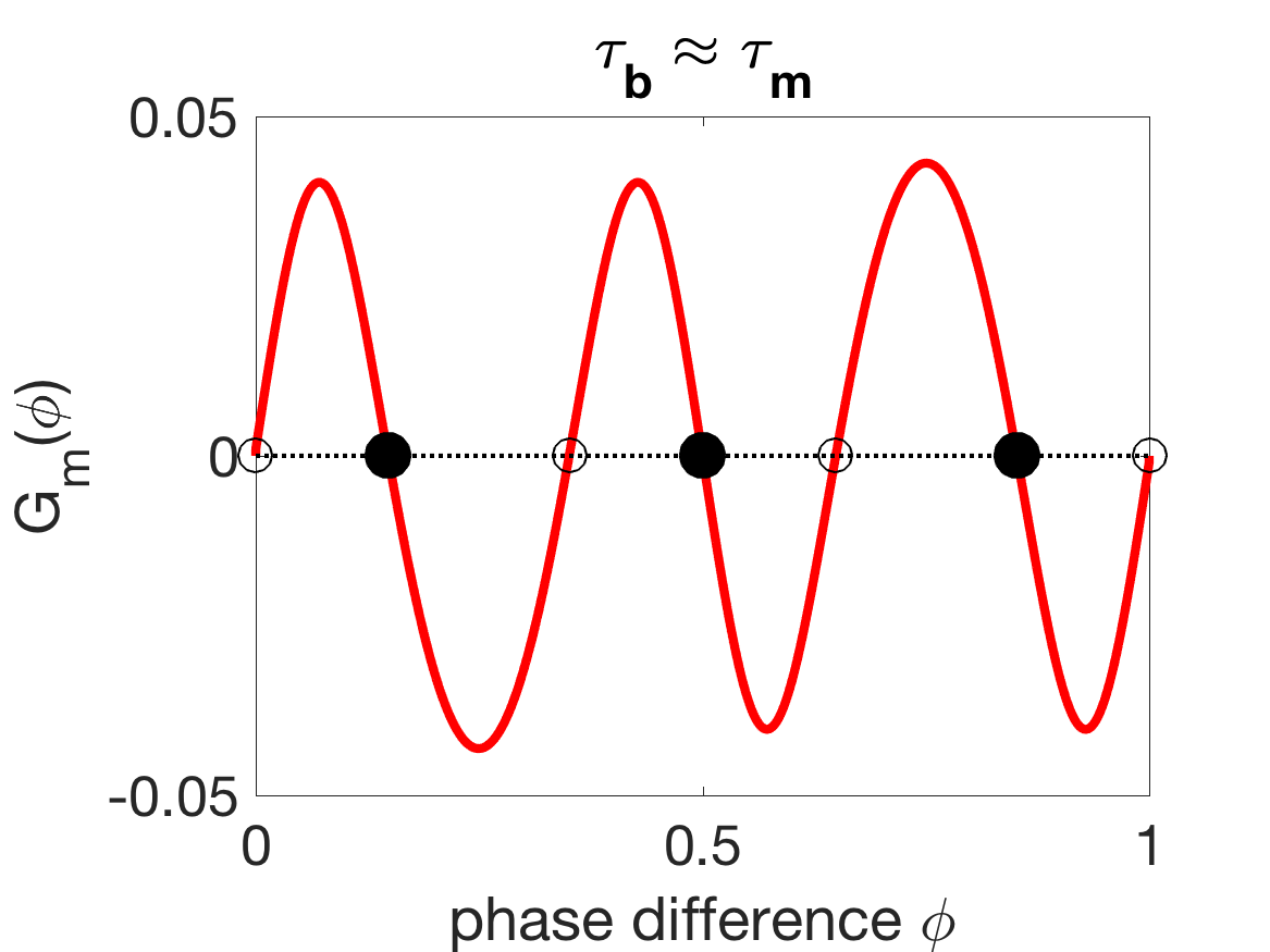 (d)
(d)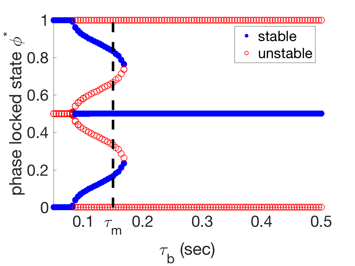
4.4 Mechanism for Gait Adaptation Holds in Six-Oscillator Case
We simulate the six-oscillator phase model in order to (i) assess the predictive power of the phase model by a quantitative comparison to the full six-module neuromechanical model and (ii) determine whether the mechanism of gait adaptation analyzed in the two-module case extends to the full six-module case.
Figure 12(a) shows the wavelengths for the six-oscillator phase model (line, circles) and neuromechanical model (crosses) as a function of external fluid viscosity for and (these coupling strengths were chosen so that the water-wavelength is approximately 1.5). The wavelengths were computed by equation 54 in Appendix A. The phase model and the neuromechanical model agree quantitatively even at high , where the mechanical coupling strength is several orders of magnitude stronger. Figure 12(b) shows the stable phase differences between neighboring modules in the six-oscillator phase model (lines, circles) and neuromechanical model (crosses) as a function of external fluid viscosity . Again, the phase model and the neuromechanical model are in quantitative agreement. Furthermore, Figure 12(b) shows that increasing fluid viscosity affects the phase-locked states in the six-oscillator case in a similar way as in the two-oscillator case. When neural coupling dominates at low viscosity, the stable phase differences are spread out near 0.9, and as fluid viscosity increases, the mechanical coupling strength increases and the stable phase differences decrease towards antiphase. However the phase differences do not reach pairwise-antiphase as in the two-oscillator case. The large variation between the phase differences across pairs of modules is due to the non-uniformity of coupling matrices , and . The modules in the middle receive stronger mechanical coupling than the modules at the boundaries; the boundary modules receive less gap-junctional coupling because they have one fewer neighboring module; and the first module gets zero nonlocal proprioceptive feedback because it has no anterior neighboring module.
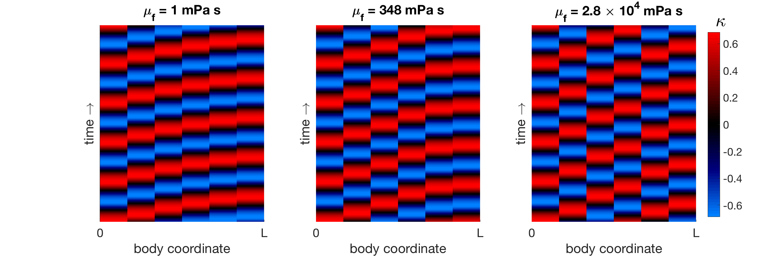
The general trend of each phase difference between neighboring modules (decreasing from near-synchrony towards antiphase) underlies the wavelength trend of gait adaptation in Figure 12(a) in both the six-oscillator phase model and the neuromechanical model. Figure 13 shows the curvature kymographs generated by the pairwise phase differences of the phase model (from Figure 12) at three selected fluid viscosities (low mPa s, medium mPa s, and high Pa s). The shortening of the wavelength seen in the curvature kymographs is a direct consequence of the decreasing pairwise phase differences. Thus, the results for the two-oscillator case in Section 4.3 extend to the six-oscillator case: the decrease in wavelength in response to increasing fluid viscosity is the result of the corresponding increase in the relative strength of mechanical coupling, which decreases the phase differences between neighboring modules and yields shorter wavelengths.
(a)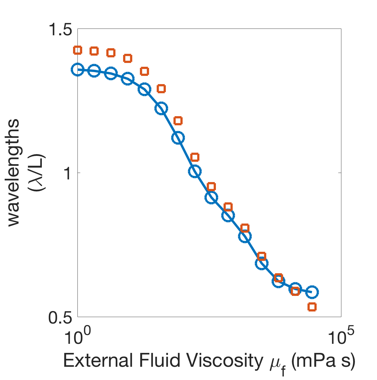 (b)
(b)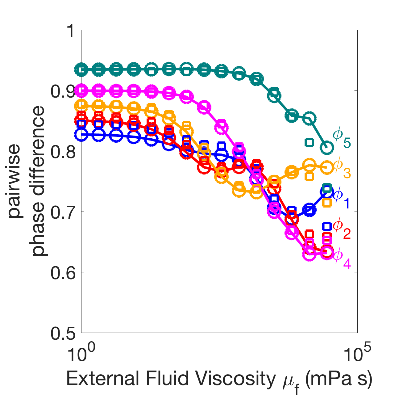
5 Discussion
The analysis of the neuromechanical model presented here identifies a mechanism for gait adaptation to increasing fluid viscosity in C. elegans forward locomotion. We model the C. elegans forward locomotion system as a chain of neuromechanical oscillators coupled by body mechanics, proprioceptive coupling, and gap-junctional coupling. Using the theory of weakly coupled oscillators, we exploit the modular structure of the forward locomotion system to analyze the relative contributions of the various coupling modalities. We find that proprioceptive coupling between modules leads to a posteriorly-directed traveling wave with a characteristic wavelength. Gap-junction coupling between neural modules promotes synchronous activity (long wavelength), and mechanical coupling promotes a high spatial frequency (short wavelength). The wavelength of C. elegans’ undulatory waveform is set by the relative strengths of these three coupling forms. As the external fluid viscosity increases, the mechanical coupling strength increases and therefore wavelength decreases, as observed experimentally.
By tuning only a few coupling parameters, the model can robustly capture the gait adaptation seen in experiments [3, 13, 40] over a wide range of mechanical parameters. The robustness of the model is of particular importance because the experimental measurements of mechanical body parameters vary widely. Our model suggests relationships between the parameters that need to hold in order to get the appropriate coordination and wavelength trend. In particular, the effective mechanical body timescale (the ratio of body viscosity to stiffness) plays a key role. Our model yields the correct coordination trend across the entire range of reported mechanical parameters, provided that is in the range s. Furthermore, the muscle activity timescale must generally be shorter than the effective body mechanics timescale . In other words, the system must generate contractile forces faster than the body responds, otherwise, there will not be a traveling wave of neuromechanical activity and therefore no effective locomotion for high external fluid viscosities. Like previous models [5], the neural timescale is assumed to be the smallest, and changing its value will likely not significantly affect the dynamics unless it is increased by an order of magnitude. However, the relative strengths of the neural coupling parameters (proprioceptive coupling strength and gap-junctional coupling strength ) are directly responsible for the appropriate coordination in the model. In particular, the long-wavelengths in the model are only achievable with sufficiently strong gap-junctional coupling.
C. elegans gait adaptation is marked by a decrease in both the wavelength and undulation frequency with increasing fluid viscosity [3, 13, 40]. Our model captures the quantitative trend in wavelength but only the qualitative trend in frequency ( Hz as opposed to the range Hz given in Fang-Yen et al. [13]). Our model is similar in structure to modeling work by Boyle et al. [5] and Denham et al. [12]. However, both Boyle et al. [5] and Denham et al. [12] are able to capture both wavelength and frequency adaptation in their models. A key difference between our model, Boyle et al. [5], and Denham et al. [12] is the role of body viscosity. In our model, the body viscosity is responsible for setting the timescale and frequency. Denham et al. [12] neglects body viscosity, so the fluid viscosity likely sets the frequency. On the other hand, Boyle et al. [5] includes an active viscosity component that depends on muscle activation, which likely provides a mechanism for frequency adaptation. In our model, body viscosity is constant, independent of muscle activation, so including an active viscosity component might be necessary for frequency adaptation.
Other differences between our model and previous models [5, 12] is the sign, directionality, and extent of nonlocal proprioception, the role of gap junctions, and the number of modules. The directionality of proprioception in Boyle et al. [5] and Denham et al. [12] is consistent with the directionality of undifferentiated processes extending posteriorly from the B-class neurons, which have postulated to be responsible for proprioception [31, 44, 48]. However, the extent of proprioception in these models needs to be much longer than this proposed biological mechanism [5, 12]. We take the directionality of proprioception to be consistent with the functional directionality suggested by the experiments of Wen et al. [43] and shown to produce locomotion in a neuromechanical model by Izquierdo and Beer [19]. Note that symmetry arguments can be made that reversing both the sign and direction of the nonlocal proprioception will not change the behavior of the models, as Denham et al. [12] points out. When we reverse the sign and direction of the nonlocal proprioception in our model, we obtain qualitatively similar results (see Appendix C). The full range of wavelength adapatation can still be achieved, and in particular the (two-module) weakly-coupled theory predicts that the change is only a small shift in the promoted phase-locked phase-difference of the proprioceptive coupling mode. The extent of proprioception in Boyle et al. [5] is over half a bodylength, and Denham et al. [12] showed that the larger the proprioceptive range, the longer the undulatory wavelength in their model. We considered only nearest-neighbor proproception because Wen et al. [43] found that proprioception likely extended anteriorly roughly 200 m or of the bodylength, similar to the length of one module in our model. This is sufficient to achieve the long-wavelength undulations in water because of our inclusion of gap-junctional coupling that promotes synchrony between the modules and thus long wavelengths. This demonstration that gap-junctions provides a mechanism for long-wavelength coordination (in the absence of long-range proprioception) is a novel contribution of this model. Furthermore in [22], we explored the effect of changing the number of modules on coordination, and we showed that gait adaptation was robustly attainable with different neural coupling strengths. Thus, the main conclusions of this paper do not depend on the number of modules considered.
Previous models which made use of more complicated mechanical and muscle models were also able to capture the swimming speed [5, 19, 12]. Here, the main purpose of our work is to determine how gait adaptation emerges from the coordination of the neuromechanical modules. Capturing the right shapes and swimming speed may involve including some of the complexities of previous models. Because we examine coordination using curvature in the small-amplitude limit, our model includes only the normal forces while tangential forces show up at higher order. Thus the tangential forces, which are important for determining swimming speed, do not affect the curvature at leading order [41].
Our model assumes that the undulatory gait emerges from a chain of neuromechanical oscillators coupled by both body mechanics and neural connectivity. However, there are several other hypotheses for how the undulatory gait is generated and coordinated [16]: (1) a separate head circuit contains a CPG that drives the propogated bending wave along the body, and (2) a network of coupled CPGs generates and coordinates the bending wave in a feed-forward manner. Modeling work by Olivares et al. [33] shows that the anatomical structure of the neural circuitry of C. elegans can be tuned to produce CPG-driven locomotion. However, there is no experimental evidence to date for such spontaneous isolated neural activity [10, 48]. Furthermore, recent experiments by [14] showed that C. elegans is capable of decoupled “two-frequency undulations”. By suppressing neural activity in the neck region, the head and body can undulate seemingly independent of one another at different frequencies (the head slower and the body faster). This evidence supports the presence of multiple neural or neuromechanical oscillators.
In the present study, the theory of weakly coupled oscillators is used to identify the roles of the various coupling modalities in generating coordination for forward locomotion in C. elegans. The phase models derived by the theory of weakly coupled oscillators capture the influence of one oscillating module on another through the interaction functions , which are convolution-like integrals of the coupling input and the corresponding phase response function of the individual modules. Therefore, our findings could be validated by experimentally measuring the phase-response curves of the neuromechanical circuit [29]. This could be achieved using a combination of optogenetic techniques and mechanical stimuli to perturb the system [14, 20, 21, 43]. Note also that the structure of the phase equations could be exploited to further dissect out the biophysical mechanisms that underlie coordination of the undulatory motion of C. elegans. Because the shapes of the PRCs and the coupling signals combine to determine the interaction functions, a systematic analysis of how cellular and synaptic dynamics [47], muscle properties, and body mechanics shape the PRCs and coupling signals would provide further insight into the integrated neuromechanical mechanisms underlying the generation and coordination of locomotion.
Appendix A Defining Wavelength
Constant Wavespeed
For a wavelength of undulation in the neuromechanical model traveling front-to-back at constant speed, the phase is defined as
| (48) |
The phase corresponding to module () centered at body position is
| (49) |
where is the oscillator period. Thus, the constant phase difference is
| (50) |
and the constant wavelength is
| (51) |
For the neuromechanical model, , so the wavelength (normalized by bodylength) is
| (52) |
Nonconstant Wavespeed
The non-uniform phase differences () between modules are used to define an effective wavelength of undulation when the wavespeed is nonconstant. The distance between the center of the first and center of the sixth module is , and the phase difference between them is . This gives an effective wavelength (normalized by 5/6 bodylengths)
| (53) |
so the wavelength (normalized by bodylength) is
| (54) |
Note that this is equivalent to the constant phase difference wavelength (equation 52) using the average phase difference between the modules as the constant phase difference , i.e., with
| (55) |
For the neuromechanical model results, first the phase differences between the modules were computed, then the wavelength was computed according to equation 54 above.
Appendix B Derivation of Mechanical Parameters
First, the bending modulus of the cuticle of the worm was determined, where is the Young’s modulus and is the second moment of area of the cuticle. The nematode body can be thought of as a pressurized, fluid-filled tube or modeled as an annular cylinder as in Cohen and Ranner [9], so the only elasticity in the body is that of the cuticle. To approximate the second moment of area of the cuticle, , note that the cuticle width m is much smaller than the average worm radius m. Following Cohen and Ranner [9],
| (56) |
The Young’s modulus has been estimated to be as small as kPa [40] or as large as MPa [13]. Backholm et al. [2] gives a range of kPa MPa. Using these estimates, we explore the range of bending moduli N(mm)2.
The cuticle viscosity has been estimated as Nm2s [13]. The internal tissue viscosity has been estimated to be constant and negative (energy-generating) as Pa s so that N(mm)2s [40] by a model fit, however this includes the active muscle components. Backholm et al. [2] estimated the range Pa s, so that the effective viscosity is N(mm)2s. These experiments used different techniques and models for viscosity, so likely have different effects lumped into the viscosity parameter. In order to explore the range of effective body mechanics timescales s, we use the range of body viscosities N(mm)2s in our model.
Appendix C Posterior-to-Anterior Proprioceptive Coupling
When we reverse the sign and direction of the nonlocal proprioception in our model, we obtain qualitatively similar results. That is, we replace the anterior-to-posterior proprioceptive coupling matrix (equation 22) with the opposite-signed, posterior-to-anterior proprioceptive coupling matrix
| (58) |
In the phase model, this yields the proprioceptive G-function (as opposed to with opposite-signed anterior-to-posterior proprioception).
Figure 14(a) shows that for particular parameters (, , , and ), the full range of wavelength adapatation can still be achieved. Note that these are smaller coupling strengths than in our standard model (this is likely due to the nonlocal proprioception here being of the same sign as the local proprioception, so it must be weaker to have less of an effect on the dynamics). In addition, the two-module weakly-coupled theory predicts that the change is only a small shift in the promoted phase-locked phase-difference of the proprioceptive coupling mode. Figure 14(b-c) shows the G-functions and corresponding phase-locked states of the proprioceptive coupling modalities. For negative, anterior-to-posterior proprioceptive coupling, the stable phase-locked state is an intermediate phase-difference (, Figure 14(b)), so the first oscillator leads the second (a front-to-back wave). Similarly, for positive, posterior-to-anterior proprioceptive coupling, the stable state is an intermediate phase-difference (, Figure 14(c)), so the first oscillator still leads the second (a front-to-back wave). Thus the change is only a small shift in the promoted phase-locked phase-difference but not a change in the direction of the traveling wave. Based on this analysis, the full neuromechanical model is likely to behave qualitatively the same for either proprioceptive mode, though a full parameter study should be done to say so definitively.
(a)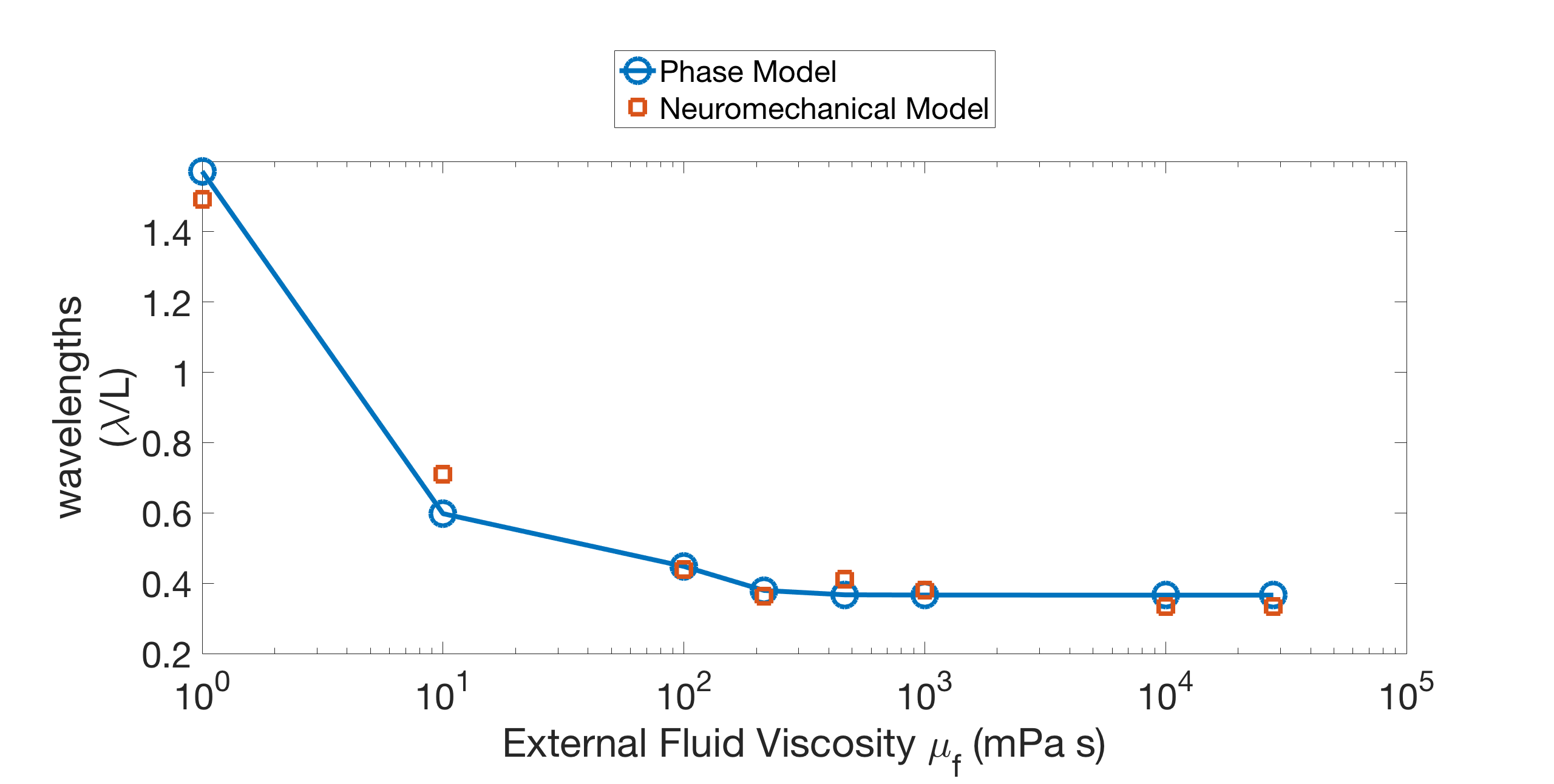
(b)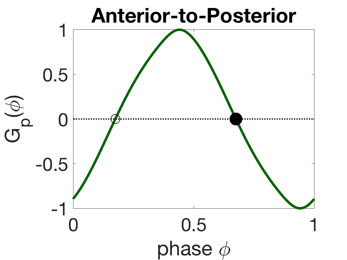 (c)
(c)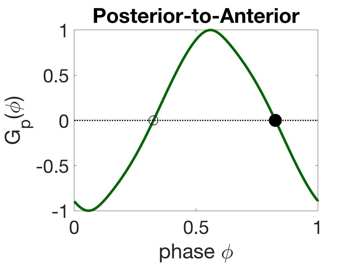
Acknowledgments
The authors would like to thank Netta Cohen for helpful discussions related to this work, as well as the reviewers for their substantial comments and suggestions. The work of RDG was partially supported by NSF grant DMS-1664679.
References
- [1] A. Ayali, A. Borgmann, A. Büschges, E. Couzin-Fuchs, S. Daun-Gruhn, and P. Holmes, The comparative investigation of the stick insect and cockroach models in the study of insect locomotion, Current Opinion in Insect Science, 12 (2015), pp. 1–10.
- [2] M. Backholm, W. S. Ryu, and K. Dalnoki-Veress, Viscoelastic properties of the nematode caenorhabditis elegans, a self-similar, shear-thinning worm, Proceedings of the National Academy of Sciences, 110 (2013), pp. 4528–4533, https://doi.org/10.1073/pnas.1219965110, http://dx.doi.org/10.1073/pnas.1219965110.
- [3] S. Berri, J. H. Boyle, M. Tassieri, I. A. Hope, and N. Cohen, Forward locomotion of the nematode c. elegans is achieved through modulation of a single gait, HFSP Journal, 3 (2009), pp. 186–193, https://doi.org/10.2976/1.3082260, http://dx.doi.org/10.2976/1.3082260.
- [4] A. Borgmann, H. Scharstein, and A. Büschges, Intersegmental coordination: Influence of a single walking leg on the neighboring segments in the stick insect walking system, Journal of Neurophysiology, 98 (2007), pp. 1685–1696, https://doi.org/10.1152/jn.00291.2007, http://dx.doi.org/10.1152/jn.00291.2007.
- [5] J. H. Boyle, S. Berri, and N. Cohen, Gait modulation in c. elegans: An integrated neuromechanical model, Front Comput Neurosci, 6 (2012), p. 10, https://doi.org/10.3389/fncom.2012.00010.
- [6] J. Bryden and N. Cohen, Neural control of caenorhabditis elegans forward locomotion: the role of sensory feedback, Biological Cybernetics, 98 (2008), pp. 339–351, https://doi.org/10.1007/s00422-008-0212-6, http://dx.doi.org/10.1007/s00422-008-0212-6.
- [7] M. Chalfie, J. E. Sulston, J. G. White, E. Southgate, J. N. Thomson, and S. Brenner, The neural circuit for touch sensitivity in caenorhabditis elegans, Journal of Neuroscience, 5 (1985), pp. 956–964.
- [8] A. H. Cohen, G. Bard Ermentrout, T. Kiemel, N. Kopell, K. A. Sigvardt, and T. L. Williams, Modelling of intersegmental coordination in the lamprey central pattern generator for locomotion, Trends in Neurosciences, 15 (1992), pp. 434–438, https://doi.org/10.1016/0166-2236(92)90006-t, http://dx.doi.org/10.1016/0166-2236(92)90006-T.
- [9] N. Cohen and T. Ranner, A new computational method for a model of c. elegans biomechanics: Insights into elasticity and locomotion performance, arXiv:1702.04988v1 [physics.bio-ph], (2017).
- [10] N. Cohen and T. Sanders, Nematode locomotion: dissecting the neuronal–environmental loop, Current Opinion in Neurobiology, 25 (2014), pp. 99–106, https://doi.org/10.1016/j.conb.2013.12.003, http://dx.doi.org/10.1016/j.conb.2013.12.003.
- [11] L. Deng, J. Denham, C. Arya, O. Yuval, N. Cohen, and G. Haspel, Inhibition underlies fast undulatory locomotion in c. elegans, eNeuro, (2020), https://doi.org/10.1523/ENEURO.0241-20.2020, https://www.eneuro.org/content/early/2020/12/14/ENEURO.0241-20.2020, https://arxiv.org/abs/https://www.eneuro.org/content/early/2020/12/14/ENEURO.0241-20.2020.full.pdf.
- [12] J. E. Denham, T. Ranner, and N. Cohen, Signatures of proprioceptive control in caenorhabditis elegans locomotion, Philosophical Transactions of the Royal Society B: Biological Sciences, 373 (2018), p. 20180208, https://doi.org/10.1098/rstb.2018.0208, http://dx.doi.org/10.1098/rstb.2018.0208.
- [13] C. Fang-Yen, M. Wyart, J. Xie, R. Kawai, T. Kodger, S. Chen, Q. Wen, and A. D. T. Samuel, Biomechanical analysis of gait adaptation in the nematode caenorhabditis elegans, Proc Natl Acad Sci U S A, 107 (2010), pp. 20323–8, https://doi.org/10.1073/pnas.1003016107.
- [14] A. D. Fouad, S. Teng, J. R. Mark, A. Liu, P. Alvarez-Illera, H. Ji, A. Du, P. D. Bhirgoo, E. Cornblath, S. A. Guan, and C. Fang-Yen, Distributed rhythm generators underlie caenorhabditis elegans forward locomotion, Elife, 7 (2018), https://doi.org/10.7554/eLife.29913.
- [15] E. Fuchs, P. Holmes, T. Kiemel, and A. Ayali, Intersegmental coordination of cockroach locomotion: adaptive control of centrally coupled pattern generator circuits, Frontiers in neural circuits, 4 (2011), p. 125.
- [16] J. Gjorgjieva, D. Biron, and G. Haspel, Neurobiology of caenorhabditis elegans locomotion: Where do we stand?, BioScience, 64 (2014), pp. 476–486, https://doi.org/10.1093/biosci/biu058, http://dx.doi.org/10.1093/biosci/biu058.
- [17] G. Haspel and M. J. O’Donovan, A perimotor framework reveals functional segmentation in the motoneuronal network controlling locomotion in caenorhabditis elegans, Journal of Neuroscience, 31 (2011), pp. 14611–14623, https://doi.org/10.1523/JNEUROSCI.2186-11.2011, http://www.jneurosci.org/content/31/41/14611, https://arxiv.org/abs/http://www.jneurosci.org/content/31/41/14611.full.pdf.
- [18] P. Holmes, R. J. Full, D. Koditschek, and J. Guckenheimer, The dynamics of legged locomotion: Models, analyses, and challenges, SIAM Review, 48 (2006), pp. 207–304, https://doi.org/10.1137/S0036144504445133, https://doi.org/10.1137/S0036144504445133, https://arxiv.org/abs/https://doi.org/10.1137/S0036144504445133.
- [19] E. J. Izquierdo and R. D. Beer, From head to tail: a neuromechanical model of forward locomotion in caenorhabditis elegans, Philosophical Transactions of the Royal Society B: Biological Sciences, 373 (2018), p. 20170374, https://doi.org/10.1098/rstb.2017.0374, http://dx.doi.org/10.1098/rstb.2017.0374.
- [20] H. Ji, A. D. Fouad, and C. Fang-Yen, A novel model of bending wave generation supports a threshold-switch mechanism in the c. elegans motor circuit, in the Proceedings of the 22nd International C. elegans Conference, 2019.
- [21] H. Ji, A. D. Fouad, S. Teng, A. Liu, P. Alvarez-Illera, B. Yao, Z. Li, and C. Fang-Yen, Phase response analyses support a relaxation oscillator model of locomotor rhythm generation in caenorhabditis elegans, bioRxiv, (2020), https://doi.org/10.1101/2020.06.22.164939, https://www.biorxiv.org/content/early/2020/06/24/2020.06.22.164939, https://arxiv.org/abs/https://www.biorxiv.org/content/early/2020/06/24/2020.06.22.164939.full.pdf.
- [22] C. L. Johnson, Neuromechanical Mechanisms of Locomotion in C. elegans, PhD thesis, University of California, Davis, 2020.
- [23] N. Kopell and G. B. Ermentrout, Symmetry and phaselocking in chains of weakly coupled oscillators, Communications on Pure and Applied Mathematics, 39 (1986), pp. 623–660, https://doi.org/10.1002/cpa.3160390504, http://dx.doi.org/10.1002/cpa.3160390504.
- [24] B. C. Ludwar, M. L. Göritz, and J. Schmidt, Intersegmental coordination of walking movements in stick insects, Journal of Neurophysiology, 93 (2005), pp. 1255–1265, https://doi.org/10.1152/jn.00727.2004, http://dx.doi.org/10.1152/jn.00727.2004.
- [25] E. Marder and R. L. Calabrese, Principles of rhythmic motor pattern generation, Physiological Reviews, 76 (1996), pp. 687–717, https://doi.org/10.1152/physrev.1996.76.3.687, http://dx.doi.org/10.1152/physrev.1996.76.3.687.
- [26] J. E. Mellem, P. J. Brockie, D. M. Madsen, and A. V. Maricq, Action potentials contribute to neuronal signaling in c. elegans, Nat Neurosci, 11 (2008), pp. 865–7, https://doi.org/10.1038/nn.2131.
- [27] B. Milligan, N. Curtin, and Q. Bone, Contractile properties of obliquely striated muscle from the mantle of squid (alloteuthis subulata) and cuttlefish (sepia officinalis), Journal of Experimental Biology, 200 (1997), pp. 2425–2436, https://jeb.biologists.org/content/200/18/2425, https://arxiv.org/abs/https://jeb.biologists.org/content/200/18/2425.full.pdf.
- [28] O. J. Mullins, J. T. Hackett, J. T. Buchanan, and W. O. Friesen, Neuronal control of swimming behavior: comparison of vertebrate and invertebrate model systems, Prog Neurobiol, 93 (2011), pp. 244–69, https://doi.org/10.1016/j.pneurobio.2010.11.001.
- [29] T. Netoff, M. Schwemmer, and T. Lewis, Phase Response Curves in Neuroscience, vol. 6 of Springer Series in Computational Neuroscience, Springer, 2012, ch. Experimentally Estimating Phase Response Curves of Neurons: Theoretical and Practical Issues.
- [30] E. Niebur and P. Erdös, Theory of the locomotion of nematodes, Biophysical Journal, 60 (1991), pp. 1132–1146, https://doi.org/10.1016/s0006-3495(91)82149-x, http://dx.doi.org/10.1016/S0006-3495(91)82149-X.
- [31] E. Niebur and P. Erdos, Theory of the locomotion of nematodes: Control of the somatic motor neurons by interneurons, Mathematical Biosciences, 118 (1993), pp. 51 – 82, https://doi.org/https://doi.org/10.1016/0025-5564(93)90033-7, http://www.sciencedirect.com/science/article/pii/0025556493900337.
- [32] V. M. Nigon and M.-A. Félix, History of research on c. elegans and other free-living nematodes as model organisms, WormBook, 2017 (2017), pp. 1–84, https://doi.org/10.1895/wormbook.1.181.1.
- [33] E. O. Olivares, E. J. Izquierdo, and R. D. Beer, Potential role of a ventral nerve cord central pattern generator in forward and backward locomotion in caenorhabditis elegans, Network Neuroscience, 2 (2018), pp. 323–343, https://doi.org/10.1162/netn_a_00036, http://dx.doi.org/10.1162/netn_a_00036.
- [34] K. G. Pearson, Generating the walking gait: role of sensory feedback, Brain Mechanisms for the Integration of Posture and Movement, (2004), pp. 123–129, https://doi.org/10.1016/s0079-6123(03)43012-4, http://dx.doi.org/10.1016/S0079-6123(03)43012-4.
- [35] W. R. Schafer, Proprioception: A channel for body sense in the worm, Current Biology, 16 (2006), pp. R509–R511, https://doi.org/10.1016/j.cub.2006.06.012, http://dx.doi.org/10.1016/j.cub.2006.06.012.
- [36] M. A. Schwemmer and T. J. Lewis, The Theory of Weakly Coupled Oscillators, Springer New York, New York, NY, 2012, pp. 3–31, https://doi.org/10.1007/978-1-4614-0739-3_1, https://doi.org/10.1007/978-1-4614-0739-3_1.
- [37] K. A. Sigvardt and T. L. Williams, Effects of local oscillator frequency on intersegmental coordination in the lamprey locomotor cpg: theory and experiment, J Neurophysiol, 76 (1996), pp. 4094–103, https://doi.org/10.1152/jn.1996.76.6.4094.
- [38] F. K. Skinner, N. Kopell, and B. Mulloney, How does the crayfish swimmeret system work? insights from nearest-neighbor coupled oscillator models, J Comput Neurosci, 4 (1997), pp. 151–60.
- [39] F. K. Skinner and B. Mulloney, Intersegmental coordination in invertebrates and vertebrates, Curr Opin Neurobiol, 8 (1998), pp. 725–32.
- [40] J. Sznitman, X. Shen, P. K. Purohit, and P. E. Arratia, The effects of fluid viscosity on the kinematics and material properties of c. elegans swimming at low reynolds number, Experimental Mechanics, 50 (2010), pp. 1303–1311, https://doi.org/10.1007/s11340-010-9339-1, https://doi.org/10.1007/s11340-010-9339-1.
- [41] B. Thomases and R. D. Guy, Mechanisms of elastic enhancement and hindrance for finite-length undulatory swimmers in viscoelastic fluids, Physical Review Letters, 113 (2014), https://doi.org/10.1103/PhysRevLett.113.098102.
- [42] E. D. Tytell, C.-Y. Hsu, T. L. Williams, A. H. Cohen, and L. J. Fauci, Interactions between internal forces, body stiffness, and fluid environment in a neuromechanical model of lamprey swimming, Proceedings of the National Academy of Sciences, 107 (2010), pp. 19832–19837, https://doi.org/10.1073/pnas.1011564107, http://dx.doi.org/10.1073/pnas.1011564107.
- [43] Q. Wen, M. D. Po, E. Hulme, S. Chen, X. Liu, S. W. Kwok, M. Gershow, A. M. Leifer, V. Butler, C. Fang-Yen, T. Kawano, W. R. Schafer, G. Whitesides, M. Wyart, D. B. Chklovskii, M. Zhen, and A. D. T. Samuel, Proprioceptive coupling within motor neurons drives c. elegans forward locomotion, Neuron, 76 (2012), pp. 750–61, https://doi.org/10.1016/j.neuron.2012.08.039.
- [44] J. G. White, E. Southgate, J. N. Thomson, and S. Brenner, The structure of the nervous system of the nematode caenorhabditis elegans, Philos Trans R Soc Lond B Biol Sci, 314 (1986), pp. 1–340.
- [45] C. H. Wiggins and R. E. Goldstein, Flexive and propulsive dynamics of elastica at low reynolds number, Physical Review Letters, 80 (1998), pp. 3879–3882, https://doi.org/10.1103/PhysRevLett.80.3879.
- [46] C. Zhang, R. D. Guy, B. Mulloney, Q. Zhang, and T. J. Lewis, Neural mechanism of optimal limb coordination in crustacean swimming, Proceedings of the National Academy of Sciences, 111 (2014), pp. 13840–13845, https://doi.org/10.1073/pnas.1323208111, http://dx.doi.org/10.1073/pnas.1323208111.
- [47] C. Zhang and T. J. Lewis, Phase response properties of half-center oscillators, Journal of Computational Neuroscience, 35 (2013), pp. 55–74, https://doi.org/10.1007/s10827-013-0440-1, http://dx.doi.org/10.1007/s10827-013-0440-1.
- [48] M. Zhen and A. D. T. Samuel, C. elegans locomotion: small circuits, complex functions, Curr Opin Neurobiol, 33 (2015), pp. 117–26, https://doi.org/10.1016/j.conb.2015.03.009.