Neutrino bound states and bound systems

Alexei Yu. Smirnov^a and Xun-Jie Xu^b ^a Max-Planck-Institut für Kernphysik, Postfach 103980, D-69029 Heidelberg, Germany
^b Institute of High Energy Physics, Chinese Academy of Sciences, Beijing 100049, China

(July 17, 2025)

Abstract

Yukawa interactions of neutrinos with a new light scalar boson $\phi$ can lead to formation of stable bound states and bound systems of many neutrinos ( $\nu$ -clusters). For allowed values of the coupling $y$ and the scalar mass $m_{\phi}$ , the bound state of two neutrinos would have the size larger than $10^{12}$ cm. Bound states with sub-cm sizes are possible for keV scale sterile neutrinos with coupling $y>10^{-4}$ . For $\nu$ -clusters we study in detail the properties of final stable configurations. If there is an efficient cooling mechanism, these configurations are in the state of degenerate Fermi gas. We formulate and solve equations of the density distributions in $\nu$ -clusters. In the non-relativistic case, they are reduced to the Lane-Emden equation. We find that (i) stable configurations exist for any number of neutrinos, $N$ ; (ii) there is a maximal central density $\sim 10^{9}$ cm^-3 determined by the neutrino mass; (iii) for a given $m_{\phi}$ there is a minimal value of $Ny^{3}$ for which stable configurations can be formed; (iv) for a given strength of interaction, $S_{\phi}=(ym_{\nu}/m_{\phi})^{2}$ , the minimal radius of $\nu$ -clusters exists. We discuss the formation of $\nu$ -clusters from relic neutrino background in the process of expansion and cooling of the Universe. One possibility realized for $S_{\phi}>700$ is the development of instabilities in the $\nu$ -background at $T<m_{\nu}$ which leads to its fragmentation. For $S_{\phi}\in[70,\,700]$ they might be formed via the growth of initial density perturbations in the $\nu$ -background and virialiazation, in analogy with the formation of Dark Matter halos. For allowed values of $y$ , cooling of $\nu$ -clusters due to $\phi$ -bremsstrahlung and neutrino annihilation is negligible. The sizes of $\nu$ -clusters may range from $\sim$ km to $\sim 5$ Mpc. Formation of clusters affects perspectives of detection of relic neutrinos.

I Introduction

In recent years neutrinos and new physics at low energy scales became one of the most active areas of research. In particular, neutrino interactions with new and very light bosons have been actively explored, with considerations covering e.g. oscillation phenomena Samanta (2011); Heeck and Rodejohann (2011); Wise and Zhang (2018); Bustamante and Agarwalla (2019); Smirnov and Xu (2019); Babu et al. (2020) and various astrophysical and cosmological consequences Boehm et al. (2012); Heeck (2014); Huang et al. (2018); Luo et al. (2021); Esteban and Salvado (2021); Green et al. (2021). Yet another possible consequence of such interactions (the subject of this paper) is the formation of bound states and bound systems of neutrinos.

The exploration of possible existence of $N$ -body bound states of neutrinos (neutrino clouds, balls, stars, or halos) has a long story. In 1964 Markov proposed the existence of “neutrino superstars” formed by massive neutrinos due to the usual gravity Markov (1964). The system is similar to neutron stars and can be described as the degenerate Fermi gas in thermodynamical and mechanical equilibrium. Substituting the mass of neutron, $m_{n}$ , by the mass of neutrino, $m_{n}\rightarrow m_{\nu}$ in results for neutron stars, Markov obtained the radius of a neutrino star:

R\simeq\sqrt{\frac{8\pi}{G_{N}}}\frac{1}{m_{\nu}^{2}},

(1)

which corresponds to the Oppenheimer-Volkoff limit. In comparison to the radius of neutron star, $R$ increases by a factor of $\beta^{2}$ where

\beta\equiv\frac{m_{n}}{m_{\nu}}=1.9\cdot 10^{10},

and for numerical estimation we take $m_{\nu}=0.05$ eV. Correspondingly, the mass of neutrino star increases and the central density decreases as

M_{\nu}\simeq\beta^{2}M_{\rm NS},\,\,\,\,\,n_{\nu}(0)\simeq\beta^{-3}n_{\rm NS}(0).

(2)

For $m_{\nu}\approx m_{e}$ used by Markov, the size, the mass and the number density of the superstars would be $R=10^{12}$ cm, $M=10^{6}M_{\odot}$ and $n_{\nu}\simeq 10^{29}\,{\rm cm}^{-3}$ correspondingly. For the present values of neutrino mass (0.1 eV), the relations (1) and (2) give

R\simeq 5\cdot 10^{26}\,{\rm cm},\,\,\,\,\,M_{\nu}=4\cdot 10^{20}M_{\odot},\,\,\,\,\,n_{\nu}(0)\simeq 10^{8}\,{\rm cm}^{-3}.

The radius is only 20 times smaller than the size of observable Universe (the present Hubble scale), and the total number of neutrinos is 10 times larger than the number of relic neutrinos in whole the Universe with the standard density. The bound states of much smaller sizes and higher densities with substantial implications for cosmology and structure formation as well as for laboratory experiments require new physics beyond the Standard Model.

One can also consider heavy (sterile) neutrinos and gravity only. Masses of $(10-100)$ keV correspond to $\beta=(10^{5}-10^{4})$ , and consequently, stars have radii of $(10^{16}-10^{14})$ cm and masses of $(10^{10}-10^{8})M_{\odot}$ , i.e. much below the galactic scales. The central density would be $(10^{24}-10^{27})\,{\rm cm}^{-3}$ . Such a possibility was explored in a series of papers Viollier et al. (1993); Bilic et al. (1999, 2001). This is essentially the warm dark matter for which final configurations of degenerate gas cannot be achieved.

Another way to reduce the size and mass of a neutrino star is to consider new long-range interactions between neutrinos which are much stronger than gravity. In the case of Yukawa forces due to a new light scalar boson $\phi$ with the coupling constant to neutrinos, $y$ , the Newton coupling $G_{N}$ should be substituted in (1) by

G_{\nu}=\frac{y^{2}}{4\pi}\frac{1}{m_{\nu}^{2}}.

(3)

As a result, we obtain

R=4\pi\sqrt{2}\frac{1}{ym_{\nu}}=\frac{17.8}{ym_{\nu}}.

(4)

Notice that this expression does not depend on the mass of mediator $m_{\phi}$ as long as $m_{\phi}\ll 1/R$ . For $y=10^{-7}$ and $m_{\nu}=0.05$ eV, one finds from (3) $\sqrt{G_{\nu}}=0.56$ MeV^-1 (that is, 22 orders of magnitude larger than $\sqrt{G_{N}}$ ), and correspondingly Eq. (4) gives $R=0.7$ km.

Properties and formation of the $\nu$ -clusters due to new scalar interactions were studied in Stephenson et al. (1998); Stephenson and Goldman (1993) using equations of Quantum Hadrodynamics. The central notion is the effective neutrino mass $\tilde{m}_{\nu}$ in the background of degenerate neutrino gas and scalar field. The equation for $\tilde{m}_{\nu}$ was obtained in the limit of static and uniform medium. This non-linear equation depends on the Fermi momentum $k_{F}$ and the strength of interactions which is defined as

G_{\phi}\equiv\frac{y^{2}\omega}{2\pi^{2}m_{\phi}^{2}}.

Here $\omega$ is the number of degrees of freedom. For large densities before neutrino clustering, the effective mass is close to zero Stephenson et al. (1998):

\tilde{m}_{\nu}\approx\frac{2m_{\nu}}{G_{\phi}k_{F}^{2}}.

At small densities: $\tilde{m}_{\nu}\rightarrow m_{\nu}$ . Using $\tilde{m}_{\nu}$ , the energy density of neutrinos, $\rho_{\nu}$ , and the energy density of the scalar field, $\rho_{\phi}$ , were computed in Stephenson et al. (1998) which gives the total energy per neutrino

\epsilon^{\rm tot}=\epsilon_{\nu}+\epsilon_{\phi}=\frac{1}{n_{F}}(\rho_{\nu}+\rho_{\phi}),

here $n_{F}=k_{F}^{3}/6\pi^{2}$ . For large enough strength $G_{\phi}$ the energy $\epsilon^{\rm tot}$ as a function of $k_{F}$ acquires a minimum with $\epsilon^{\rm tot}<m_{\nu}$ around $k_{F}^{\min}\approx 0.8m_{\nu}$ . Clustering of neutrinos starts when $k_{F}$ decreases due to the expansion of the Universe down to

k_{F}\sim k_{F}^{\min}.

It is also assumed that with the expansion (decrease of $n$ ), the kinetic energy could be converted into the increasing effective mass $\tilde{m}_{\nu}$ and the gas became strongly degenerate.

To describe finite size objects, the static equations of motion were used with non-zero spatial derivatives of the fields, and consequently, $\tilde{m}_{\nu}$ . It was assumed that the distribution of clusters on the number of neutrinos $N$ follows the density fluctuations and has the Harrison-Zeldovich spectrum. In Stephenson et al. (1998), the neutrino mass $m_{\nu}=13$ eV motivated by the Tritium experiment anomaly was used. Very small mediator masses $m_{\phi}\sim 10^{-17}$ eV and couplings $g\sim 10^{-14}$ were taken. Consequently, the sizes of clusters equal $\sim 10^{13}$ cm, which is roughly the size of the Earth orbit, and the central densities could reach $10^{15}$ cm^-3.

Later the bound systems of heavy Dirac fermions (“nuggets”) due to Yukawa couplings with light or massless scalar were explored Wise and Zhang (2014, 2015); Gresham et al. (2017, 2018). With fermion masses $m_{D}\sim 100$ GeV and coupling $\alpha_{\phi}\sim(0.01-0.1)$ such systems were applied to the Asymmetric Dark Matter (ADM). The description of nuggets in Wise and Zhang (2015), Gresham et al. (2017) is similar to that of neutrino stars Stephenson et al. (1998)¹¹1 The authors of those ADM papers overlooked (and do not refer to) similar papers on neutrinos Stephenson et al. (1998) published 20 years before. In the first version of our paper we, being focussed on neutrinos, overlooked the papers on ADM.. The effective mass of fermion was introduced as in Stephenson et al. (1998) and equations for its dependence on $r$ was derived. The system of equations for the scalar field and Fermi momentum of ADM particles $p_{F}(r)$ (and therefore their density) was presented. In Wise and Zhang (2015) the equations were solved by introducing an ansatz for $p_{F}(r)$ , thus reducing the system to a single equation. In Gresham et al. (2017) the complete system of equations was solved numerically. Dependence of properties of nuggets on $N$ , in particular $R(N)$ , were studied. It was established in Wise and Zhang (2015) that with the increase of $N$ the radius first decreases, reaches minimum and then increases. The increase is associated to transition from non-relativistic to relativistic regime. While in Wise and Zhang (2015) the mediator was assumed to be massless, in Gresham et al. (2017) dependence of characteristics of nuggets on $m_{\phi}$ was studied and, in particular, the case of “saturation”, which corresponds to $R>1/m_{\phi}$ , was noticed.

Due to strongly different values of masses and coupling constant the formation and cosmological consequences of nuggets are completely different from those of neutrino stars. Also observational methods and perspectives of detection are different. Our paper is continuation of the work in Stephenson et al. (1998) for neutrinos. Where possible, we compare our results with those for ADM.

We perform a systematic study of various aspects of physics of neutrino clusters. The paper contains a number of derivations and auxiliary material which will be useful for further studies and applications.

In this paper, we revisit the possibility of formation of the neutrino bound states and bound systems due to neutrino interactions with very light scalar bosons. First the bound states of two neutrinos are considered. We formulate conditions for their existence and find their parameters such as eigenstates and eigenvalues. For usual neutrinos and allowed values of $y$ and $m_{\phi}$ , the sizes of these bound states are of the astronomical distances which has no sense. For sterile neutrinos with mass $m_{\nu}\geq 10$ keV and $y>10^{-4}$ the size can be in sub-cm range and formation of such states may have implications for dark matter.

Then we study properties and formation of the $N$ -neutrino bound systems — the $\nu$ -clusters with a sufficiently large $N$ , so that the system can be quantitatively described using Fermi-Dirac statistics. We compute characteristics of possible stable final configurations of the $\nu$ -clusters as function of $N$ — mostly in the state of degenerate Fermi gas (ground state) but also with thermal distributions. Energy loss of the $\nu$ -clusters is estimated. Depending on $N$ (we explore the entire possible range) the clusters can be in non-relativistic or relativistic regimes and we study the transition between these two regimes. In the non-relativistic case, using equations of motions for $\nu$ and $\phi$ , we rederive the Lane-Emden equation for the neutrino density. We obtain qualitative analytic results for parameters of the neutrino cluster. The equation for the relativistic case is derived which is similar to the one used in Stephenson et al. (1998). We use presently known values of neutrino masses which are two orders of magnitude smaller than in Stephenson et al. (1998), and consequently, parameters of the clouds are different.

Understanding the formation of neutrino clusters from homogeneous relativistic neutrino gas requires numerical simulations. In this connection we present some relevant analytic results. One possible mechanism of formation is the development of instabilities in the uniform neutrino background, which leads to fragmentation and further redistribution of neutrino density, thus approaching final degenerate configurations. In some parameter space, one can use an analogy between Yukawa forces and gravity and therefore compare it with the formation of dark matter halos due to gravity.

The paper is organized as follows. We start with re-derivation of the Yukawa potential in Sec. II, where we adopt the approach developed in Ref. Smirnov and Xu (2019) and generalize it to the relativistic case. In Sec. III, we study the two-body bound states in the framework of quantum mechanics. In Sec. IV, the $N$ -body bound systems are considered. The results of Sec. III and Sec. IV apply to the non-relativistic neutrinos, while a study of the relativistic case is presented in Sec. V. In Sec. VI, we speculate on possible mechanisms of formation of the $\nu$ -clusters which include fragmentation of the cosmic neutrino background induced by the expansion of the Universe. Further evolution and formation of final configurations are outlined. Energy loss of the clusters is estimated. Analogy with formation of DM halos is outlined. Finally, we conclude in Sec. VII. Various details and explanations are presented in the appendices.

II Yukawa potential for neutrinos

In general, to form a bound state, the range of the force, $R_{{\rm force}}$ , needs to be longer than the de Broglie wavelength of the neutrino, $\lambda_{\nu}$ :

R_{{\rm force}}>\lambda_{\nu}.

(5)

For a non-relativistic neutrino $\lambda_{\nu}=(m_{\nu}v)^{-1}$ , where $v$ is the neutrino velocity, and $R_{{\rm force}}\sim 1/n_{\phi}$ is given by the inverse of the mediator mass. Therefore Eq. (5) can be written as $m_{\phi}<m_{\nu}v$ , which implies that mediator should be lighter than the neutrino to form a bound state²²2In the standard model (SM), the $Z$ boson does mediate an attractive force between a neutrino and an antineutrino but due to its large mass, the range of this force is too short to bind neutrinos together..

Let us consider a light real scalar boson $\phi$ interacting with neutrinos

{\cal L}=\frac{1}{2}\partial^{\mu}\phi\partial_{\mu}\phi-\frac{1}{2}m_{\phi}^{2}\phi^{2}+\overline{\nu}i\not{\partial}\nu-m_{\nu}\overline{\nu}\nu-y\overline{\nu}\phi\nu.

(6)

We assume $m_{\phi}\ll m_{\nu}$ , so that $\nu$ can be treated as point-like particles while $\phi$ as a classical field. This is valid as long as we are not concerned with hard scattering processes. In this regime, the effect of the $\phi$ field on $\nu$ particles can be described using Yukawa potential.

From Eq. (6), we obtain the Euler-Lagrange equations of motion (EOM) for $\nu$ and $\phi$ :

	$\displaystyle i\not{\partial}\nu-(m_{\nu}+y\phi)\nu$	$\displaystyle=0\thinspace,$		(7)
	$\displaystyle(\partial^{2}+m_{\phi}^{2})\phi+y\overline{\nu}\nu$	$\displaystyle=0\thinspace.$		(8)

According to Eq. (7) the effect of the $\phi$ field on the motion of $\nu$ can be accounted by shifting its mass:

\tilde{m}_{\nu}\equiv m_{\nu}+V,\ \leavevmode\nobreak\ \leavevmode\nobreak\ \leavevmode\nobreak\ \leavevmode\nobreak\ \leavevmode\nobreak\ V\equiv y\phi\thinspace.

(9)

Here $V$ is the potential, and $\tilde{m}_{\nu}$ is treated as the effective mass of neutrino in background.

At quantum level $\overline{\nu}\nu$ is replaced by the expectation value computed as (see Appendix A):

\overline{\nu}\nu\rightarrow\langle\overline{\nu}\nu\rangle=\int\frac{d^{3}\mathbf{p}}{(2\pi)^{3}}\frac{\tilde{m}_{\nu}}{E_{\mathbf{p}}}f(t,\ \mathbf{x},\ \mathbf{p})\thinspace,

(10)

where $E_{\mathbf{p}}=\sqrt{\tilde{m}_{\nu}^{2}+|\mathbf{p}|^{2}}$ and $f(t,\ \mathbf{x},\ \mathbf{p})$ is the neutrino distribution function normalized in such a way that the number density, $n$ , and the total number of $\nu$ , $N$ , are given by

n=\int f(t,\ \mathbf{x},\ \mathbf{p})\frac{d^{3}\mathbf{p}}{(2\pi)^{3}}\thinspace,\ \ N=\int n(t,\ \mathbf{x})d^{3}\mathbf{x}\thinspace.

In the non-relativistic case, $\tilde{m}_{\nu}/E_{\mathbf{p}}\approx 1$ , Eq. (10) gives

\langle\overline{\nu}\nu\rangle\approx n.

(11)

We assume a static distribution, so that $\partial_{t}\phi=0$ . Replacing $\overline{\psi}\psi$ by $\langle\overline{\psi}\psi\rangle\approx n$ in Eq. (8) and using relation $\phi=V/y$ , (see Eq. (9)) we obtain equation for the potential

\left[\nabla^{2}-m_{\phi}^{2}\right]V=y^{2}n.

(12)

For spherically symmetric distribution of neutrinos, $n=n(r)$ , where $r$ is the distance from the center, Eq. (12) can be solved analytically Smirnov and Xu (2019), giving

V=-\frac{y^{2}}{m_{\phi}r}\left[e^{-m_{\phi}r}\int_{0}^{r}dr^{\prime}r^{\prime}n(r^{\prime})\sinh(m_{\phi}r^{\prime})+\sinh(m_{\phi}r^{\prime})\int_{r}^{\infty}dr^{\prime}e^{-m_{\phi}r^{\prime}}r^{\prime}n(r^{\prime})\right].

(13)

For $n=N\delta^{3}(\mathbf{x})$ (all neutrinos are in origin) the solution reproduces the Yukawa potential

V(r)=-N\frac{y^{2}}{4\pi}\frac{1}{r}e^{-rm_{\phi}}.

(14)

Note that $V$ is the potential experienced by a given neutrino, and for two neutrinos separated by a distance $r$ , the total binding energy is given by Eq. (14) with $N=1$ (see Appendix B for details).

For relativistic neutrinos, if $\partial_{t}\phi$ can be neglected³³3The time derivative $\partial_{t}\phi$ can only be neglected for stationary (e.g. the ground state of a binary system) or approximately stationary distributions (e.g., a many-body system with a low temperature). Otherwise, $\partial_{t}\phi$ plays an important role in quantum state transitions or in energy loss of a many-body system due to emission of $\phi$ waves. This is similar to the familiar example of an excited atom that will undergo transition to the ground state in finite time via spontaneous emission of electromagnetic waves., one should use general expression in (10) and the equation for the potential becomes

\left[\nabla^{2}-m_{\phi}^{2}\right]V=y^{2}\int\frac{d^{3}\mathbf{p}}{(2\pi)^{3}}\frac{\tilde{m}_{\nu}}{E_{\mathbf{p}}}f(\mathbf{x},\ \mathbf{p}).

(15)

The resulting $V$ is suppressed by a factor of $\tilde{m}_{\nu}/E_{\mathbf{p}}$ in comparison to the non-relativistic case. This equation can be written in the form Eq. (12) with $n$ substituted by the effective number density, $\tilde{n}$ , defined as

\tilde{n}\equiv\int\frac{d^{3}\mathbf{p}}{(2\pi)^{3}}\frac{\tilde{m}_{\nu}}{E_{\mathbf{p}}}f(\mathbf{x},\ \mathbf{p}).

In the non-relativistic case $\tilde{n}\rightarrow n$ .

In this paper we focus on the real scalar field. Pseudo-scalar mediators (e.g. the majoron) cause spin-dependent forces, and the corresponding potential can be found in Chikashige et al. (1981). For a two-body system, the potential might be able to bind the pair if the mediator mass is sufficiently light. In an $N$ -body system with large $N$ , the effect of spin-dependent forces is suppressed by spin averaging.

In the case of a complex scalar, our analysis can be applied to its real part, while the effect of its imaginary part, which is a pseudo-scalar, can be neglected if the two parts have the same mass. In models with spontaneous symmetry breaking such as the one in Chikashige et al. (1981), only the pseudo-scalar component is massless and therefore leads to long-range effects.

III Two-neutrino bound states

In this section, we consider bound states of two non-relativistic neutrinos due to the attractive $\phi$ potential. For DM particles this was considered in a number of papers before (see Wise and Zhang (2014) and references therein).

The strength of the interaction required to form bound states can be estimated in the following way. If the wave function of the bound state is localized in the region of radius $R$ , then according to the Heisenberg uncertainty principle the momentum of neutrino is $p\sim 1/R$ , and consequently, the kinetic energy, $E_{kin}\approx p^{2}/2m_{\nu}$ , equals

E_{{\rm kin}}\sim\frac{1}{2m_{\nu}}\frac{1}{R^{2}}.

(16)

The condition of neutrino trapping in the potential $V$ reads

E_{{\rm kin}}\lesssim-V,\ \,\,(r<R).

(17)

Plugging $E_{{\rm kin}}$ from Eq. (16) and $V$ from Eq. (14) with $N=1$ into this equation we obtain

\frac{1}{2m_{\nu}}\lesssim\frac{y^{2}R}{4\pi}e^{-Rm_{\phi}}.

(18)

Maximal value of the r.h.s. of this equation equals $y^{2}/(4\pi em_{\phi})$ , which is achieved at $R=m_{\phi}^{-1}$ . Then, according to (18), the sufficient condition for existence of bound state can be written as

\lambda\equiv\frac{y^{2}}{8\pi}\frac{m_{\nu}}{m_{\phi}}\gtrsim 0.7,

(19)

where $\lambda$ can be interpreted as strength of interaction. Quantitative study below gives $\lambda>0.84$ . The condition can be rewritten as the upper bound on $m_{\phi}$ :

m_{\phi}\lesssim\frac{y^{2}}{4\pi}m_{\nu}=4\cdot 10^{-17}\left(\frac{y}{10^{-7}}\right)^{2}{\rm eV}.

III.1 Quantitative study

Refer to caption — Figure 1: The radial dependences of the wave functions of neutrino bound states for different values of the interaction strength $\lambda$ defined in Eq. (19). In all the panels we take the orbital momentum $l=0$ . For $\lambda=0.5$ , since no bound states can be formed, we plot the wave function with the lowest energy.

Quantitative treatment of neutrino bound states requires solution of the two-body Schrödinger equation. Let $\mathbf{r}_{1}$ and $\mathbf{r}_{2}$ be the coordinates of two neutrinos. The potential depends on the relative distance between neutrinos $\mathbf{r}\equiv\mathbf{r}_{1}-\mathbf{r}_{2}$ only. Consequently, the wave function of bound state depends on $\mathbf{r}$ , $\nu=\nu(\mathbf{r})$ , and it obeys the Schrödinger equation

\left[-\frac{1}{m_{\nu}}\nabla^{2}+V(r)\right]\nu(\mathbf{r})=E\nu(\mathbf{r}),\\

(20)

with $V(r)=V(r,N=1)$ given in Eq. (14), $r=|\mathbf{r}|$ and $E$ being the energy eigenvalue. The numeric coefficient of the kinetic term takes into account the reduced mass of neutrino (see Appendix C). Since the potential $V(r)$ is independent of the direction, the wave function can be factorized as

\nu=\frac{u(r)}{r}Y_{l}^{m}(\theta,\ \varphi).

(21)

Here $u(r)$ is a radial component and $Y_{l}^{m}(\theta,\ \varphi)$ is a spherical harmonic function. Plugging Eq. (21) into Eq. (20), we obtain the equation for $u(r)$ :

-\frac{1}{m_{\nu}}\frac{d^{2}u(r)}{dr^{2}}+\left[V(r)+\frac{1}{m_{\nu}}\frac{l(l+1)}{r^{2}}\right]u(r)=Eu(r).

For zero angular momentum, $l=0$ , the equation simplifies further:

-u^{\prime\prime}(r)+m_{\nu}V(r)u(r)=m_{\nu}Eu(r).

(22)

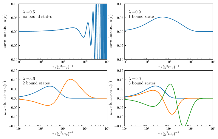
We solve this equation numerically (see details in Appendix C). $u(r)$ for different values of $\lambda$ are shown in Fig. 1. According to this figure there is no bound state for $\lambda=0.5$ : the solution with the lowest energy level does not converge to zero when $r\rightarrow\infty$ . For other specific values, $\lambda=0.9$ , $3.6$ , and $9.0$ , the figure shows one, two, and three bound states. With further increase of $\lambda$ , the number of allowed energy levels of increases. Varying $\lambda$ we find that for

•

$\lambda<0.84$ , no bound states can be formed;
•

$0.84<\lambda<3.2$ , there is one bound state (the 1s state);
•

$3.2<\lambda<7.2$ , two bound states with $l=0$ (the 2s state) can be formed;
•

$\lambda>7.2$ , three or more bound states exist, including states with $l\neq 0$ .

III.2 Coulomb limit

The limit of $m_{\phi}\rightarrow 0$ ( $\lambda\rightarrow\infty$ ) corresponds to a Coulomb-like potential, and in this case, the Schrödinger equation (22) can be solved analytically. There is an infinite number of levels and the wave function of ground state equals

u(r)=2R_{0}^{3/2}r\exp\left(-\frac{r}{R_{0}}\right),

(23)

where

R_{0}\equiv\frac{8\pi}{m_{\nu}y^{2}}\thinspace

(24)

is the radius of the bound state, and the corresponding eigenvalue equals

E=-\frac{y^{4}m_{\nu}}{64\pi^{2}}\thinspace.

(25)

This $E$ can be interpreted as the binding energy of the state. For non-zero $m_{\phi}$ such that $R_{0}\ll m_{\phi}^{-1}$ (equivalent to $\lambda\gg 1$ ), the range of the force is much larger than the radius of the bound state in the Coulomb limit. In this case, Eq. (24) and (25) can be used as a good approximation. The correction to the Coulomb limit result due to non-zero $m_{\phi}$ can be computed using the variation principle (see below).

III.3 Approximate solutions for non-zero mass of scalar from the variation principle

According to the variation principle the expectation of the Hamiltonian

\langle H\rangle\equiv\frac{\int u^{*}(r)Hu(r)\thinspace dr}{\int u^{*}(r)u(r)\thinspace dr}

reaches the minimal value when $u$ is the wave function of the ground state, while $\langle H\rangle$ itself gives the corresponding eigenvalue. The Hamiltonian for the radial wave function and $l=0$ reads

H=-\frac{1}{m_{\nu}}\frac{d^{2}}{dr^{2}}+V(r)\thinspace.

Assuming solution in the form Eq. (23): $u(r)=2a^{3/2}re^{-r/a}$ with $a$ being a free parameter, we find

\langle H\rangle=\frac{1}{a^{2}m_{\nu}}\left[1-\frac{ay^{2}m_{\nu}}{\pi(am_{\phi}+2)^{2}}\right].

(26)

Minimization of $\langle H\rangle$ with respect to $a$ , that is $d\langle H\rangle/da=0$ , gives

(16\pi\lambda+am_{\nu}y^{2})^{3}-32\pi\lambda^{2}am_{\nu}y^{2}(16\pi\lambda+3am_{\nu}y^{2})=0,

(27)

which is a cubic equation with respect to $a$ . The cubic equation has one negative solution which can be ignored, and two others which can be either both complex (in this case the two solutions are conjugate to each other) or both real and positive (in this case the two solutions are identical). Only the later case leads to a physical solution and requires that the discriminant is positive:

\lambda^{2}+\frac{20}{9}\lambda-3\geq 0\thinspace.

From this inequality we obtain

\lambda\geq\frac{1}{9}\left(7\sqrt{7}-10\right)\approx 0.95\thinspace,

which is about 13% larger than the exact value $0.84$ obtained in Sec. III.1. In Wise and Zhang (2014) the bound $\lambda\geq 0.84$ was also obtained.

Using the variation principle in this way may not give an accurate wave function, but usually leads to a very accurate result for eigenvalues Griffiths (2016). Note that here we do not require that $\lambda^{-1}\propto m_{\phi}$ is perturbatively small. For very small $\lambda^{-1}$ the result is expected to be more accurate. The series expansion of the positive physical solution of Eq. (27) in $\lambda^{-1}$ gives

x=8\pi\left[1+\frac{3}{4\lambda^{2}}+{\cal O}\left(\frac{1}{\lambda^{3}}\right)\right].

Therefore, the radius of the system $R=a=x/y^{2}m_{\nu}$ equals

R\approx\frac{8\pi}{m_{\nu}y^{2}}\left[1+\frac{3}{4\lambda^{2}}\right].

The eigenvalue is corrected according to (26) as

E=\langle H\rangle\approx-\frac{y^{4}m_{\nu}}{64\pi^{2}}\left[1-\frac{2}{\lambda}+\frac{3}{2\lambda^{2}}\right].

(28)

The lowest order expressions for $R$ and binding energy (28) coincide with those in Wise and Zhang (2014).

Numerically, the radius equals

R=5\cdot 10^{11}{\rm cm}\left(\frac{0.1{\rm eV}}{m_{\nu}}\right)\left(\frac{10^{-7}}{y}\right)^{2}.

(29)

This is much larger than the distance between relic neutrinos (without clustering) $\sim 0.16$ cm, and therefore existence of bound states of such size has no practical sense.

For two-body bound states, it is impossible to enter the relativistic regime. Indeed, according to Eq. (25) or Eq. (28) the kinetic energy being of the order of binding energy equals $y^{4}m_{\nu}/64\pi^{2}$ . Therefore the relativistic case, $E_{\rm kin}/m_{\nu}\geq 1$ implies $y\gtrsim(64\pi^{2})^{1/4}$ which would not only violate the perturbativity bound but also be excluded by various experimental limits — see Appendix D.

The results of this section may have applications for sterile neutrinos with mass $m_{\nu}\geq 10$ keV. These neutrinos could compose dark matter of the Universe. For $m_{\nu}\geq 10$ keV and $y=10^{-3}$ we find from (29) $R=0.05$ cm.

IV $N$ -neutrino bound systems

Let us consider $N$ neutrinos trapped in the Yukawa potential with $N$ being large enough, so that neutrinos form a statistical system which is described by the Fermi-Dirac distribution function

f=\frac{1}{\exp\frac{E-\mu}{T}+1}.

(30)

Here $E$ is the total neutrino energy, $\mu$ is the chemical potential and $T$ is the temperature. Recall that for this distribution the number density, $n$ , the energy density, $\rho$ , and pressure ${\cal P}$ of the system equal respectively

n=\int f\frac{d^{3}\mathbf{p}}{(2\pi)^{3}}\thinspace,\,\,\,\,\rho=\int Ef\thinspace\frac{d^{3}\mathbf{p}}{(2\pi)^{3}}\thinspace,\,\,\,\,{\cal P}=\frac{1}{3}\int\frac{|\mathbf{p}|^{2}}{E}f\thinspace\frac{d^{3}\mathbf{p}}{(2\pi)^{3}}\thinspace.

The ground state of this system ( $T\rightarrow 0$ ) is the degenerate Fermi gas with distribution $f(p)=1$ , if $E<\mu$ , and $f(p)=0$ if $E>\mu$ according to Eq. (30). (The case of finite $T$ will be discussed in Sec. VI). Consequently, in the degenerate state

n=\int_{0}^{p_{F}}\frac{4\pi p^{2}dp}{(2\pi)^{3}}=\frac{p_{F}^{3}}{6\pi^{2}}\thinspace,

(31)

and the total number of neutrinos $N$ for uniform distribution in the sphere of radius $R$ equals

N=\frac{2p_{F}^{3}}{9\pi}R^{3}\thinspace.

(32)

Eq. (31) applies to both relativistic and non-relativistic cases. For $\rho$ and ${\cal P}$ , the non-relativistic results are

{\cal P}_{\rm deg}=\frac{1}{6\pi^{2}}\int_{0}^{p_{F}}\frac{p^{2}}{E}p^{2}dp=\frac{p_{F}^{5}}{30\pi^{2}m_{\nu}}\thinspace,\,\,\,\ \rho=\frac{3}{2}{\cal P},

(33)

while the relativistic results can be obtained by computing the integrals numerically.

IV.1 Qualitative estimation

Let us consider $N$ neutrinos uniformly distributed in a sphere of radius $R$ . The Yukawa attraction produces a pressure, ${\cal P}_{{\rm Yuk}}$ , which for $m_{\phi}=0$ can be estimated as

{\cal P}_{{\rm Yuk}}\simeq\frac{1}{{\cal V}}\left[-\frac{1}{2}\frac{y^{2}N^{2}}{4\pi R}\right]\thinspace,

(34)

where ${\cal V}=\frac{4}{3}\pi R^{3}$ is the volume and the quantity in the brackets is the total potential energy.

Static configuration corresponds to the equilibrium between this Yukawa pressure and the pressure of degenerate fermion gas (Pauli repulsion):

{\cal P}_{{\rm deg}}\simeq{\cal P}_{{\rm Yuk}}\thinspace.

Using Eq. (33) and Eq. (34) this equality can be rewritten as

\frac{p_{F}^{5}}{30\pi^{2}m_{\nu}}\simeq\frac{3y^{2}N^{2}}{2\left(4\pi\right)^{2}R^{4}}\thinspace.

(35)

Inserting Eq. (32) in Eq. (35) we find

R\simeq\frac{8}{y\sqrt{m_{\nu}p_{F}}}\thinspace.

(36)

Alternatively, we can express $p_{F}$ in terms of $N$ and obtain

R\simeq\frac{30}{m_{\nu}y^{2}}\left(\frac{1}{N}\right)^{1/3}\thinspace.

(37)

Plugging $R$ from Eq. (37) back into Eq. (32), we obtain a relation between $N$ and $p_{F}$ :

N\simeq\frac{40}{y^{3}}\left(\frac{p_{F}}{m_{\nu}}\right)^{3/2}\thinspace.

(38)

Notice that for $N\rightarrow 2$ , Eq. (37) recovers approximately the result in Eq. (24) for the two-body system. A noteworthy feature of Eq. (37) is that the radius decreases with $N$ : $R\propto N^{-1/3}$ . This implies that increasing $N$ leads to a more compact cluster. This dependence is valid only in the non-relativistic regime. When $N$ is too large, the Fermi momentum $p_{F}$ which increases with $N$ according to Eq. (38) will exceed $m_{\nu}$ and the system enters the relativistic regime. As we will show in Sec. V, in the relativistic regime, the attractive force becomes suppressed, causing $R$ to increases with $N$ .

IV.2 Quantitative study

In an object of finite size, the density and pressure depend on distance from the center of object. The dependence can be obtained using the differential (local) form of the equality of forces, which is given by the equation of hydrostatic equilibrium. For degenerate neutrino gas it is reduced to the Lane-Emden (L-E) equation Chandrasekhar and Chandrasekhar (1957). The L-E equation can be also derived from equations of motion of the fields (see Appendix F).

The equation of hydrostatic equilibrium expresses the equality of the repulsive force due to the degenerate pressure, $F_{{\rm deg}}$ , and the Yukawa attractive force, $F_{\text{Yuk}}$ , acting on a unit of volume at distance $r$ from the center:

F_{{\rm deg}}(r)\equiv\frac{d{\cal P}_{{\rm deg}}(r)}{dr}=F_{\text{Yuk}}(r)\thinspace.

(39)

For non-relativistic neutrinos, ${\cal P}_{{\rm deg}}$ is given in Eq. (33), and using Eq. (31), ${\cal P}_{{\rm deg}}$ can be rewritten as

{\cal P}_{{\rm deg}}=Kn^{5/3},\,\,\,\ K\equiv\frac{(6\pi^{2})^{5/3}}{30\pi^{2}m_{\nu}}=\frac{(6\pi^{2})^{2/3}}{5m_{\nu}}\thinspace.

(40)

The Yukawa force equals

F_{{\rm Yuk}}(r)=-\frac{y^{2}}{4\pi r^{2}}n(r)N(r)\thinspace,

(41)

where

N(r)=\int_{0}^{r}dr^{\prime}4\pi r^{\prime}{}^{2}n(r^{\prime})

is the number of neutrinos inside a sphere of radius $r$ . Inserting Eqs. (40) and (41) into Eq. (39) gives the equation for $n(r)$ :

\frac{5}{3}Kn^{2/3}\frac{dn}{dr}=\frac{y^{2}}{r^{2}}n\int_{0}^{r}dr^{\prime}r^{\prime 2}n(r^{\prime})\thinspace.

Dividing this equation by $n/r^{2}$ and then differentiating by $r$ , we obtain

\frac{5}{2}K\frac{d}{dr}\left[r^{2}\frac{dn^{2/3}}{dr}\right]=-y^{2}r^{2}n\thinspace,

\frac{1}{r^{2}}\frac{d}{dr}\left[r^{2}\frac{dn^{2/3}}{dr}\right]=-y^{2}\kappa n\thinspace,

(42)

where

\kappa\equiv\frac{2m_{\nu}}{(6\pi^{2})^{2/3}}\thinspace.

Eq. (42) is nothing but the Lane-Emden equation Chandrasekhar and Chandrasekhar (1957) for specific values of parameters. In particular, $\gamma$ , defined as the ratio of powers of $n$ in the r.h.s. and the l.h.s. of Eq. (42), equals $\gamma=1/(2/3)=3/2$ . For this value the $N$ -body system has a finite size $R$ defined by

n(R)=0.

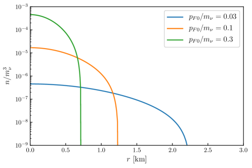
We solve the L-E equation (42) numerically with the boundary condition

n(r=0)=n_{0},\leavevmode\nobreak\ \leavevmode\nobreak\ {\rm or\leavevmode\nobreak\ \leavevmode\nobreak\ equivalently},\leavevmode\nobreak\ \leavevmode\nobreak\ p_{F}(r=0)=p_{F0}.

Fig. 2 shows solutions of $n(r)$ for different values of $p_{F0}/m_{\nu}$ . As $r$ increases, the number densities drop down to zero at

R\approx\frac{19.9}{y\sqrt{m_{\nu}p_{F0}}}.

(43)

Integrating $n(r)$ with $r$ ranging from $0$ to $R$ gives the total number of neutrinos:

N\approx\frac{93.6}{y^{3}}\left(\frac{p_{F0}}{m_{\nu}}\right)^{3/2}\thinspace.

(44)

Combining Eqs. (43) and (44), we obtain expression for the radius

R\approx\frac{90.4}{m_{\nu}y^{2}}\left(\frac{1}{N}\right)^{1/3}\thinspace,

(45)

which shows that $R$ decreases with $N$ , in agreement with the qualitative estimations in Sec. IV.1. The results in Eqs. (43), (44) and (45) have the same parametric dependence as Eqs. (36), (38) and (37) and differ by numerical factors 2.5, 2.3 and 3 correspondingly.

Notice that for the Fermi momentum $p_{F0}\sim m_{\nu}$ the Eq. (43) gives $R=19.9/ym_{\nu}$ , which practically coincides with (4) obtained from rescaling of parameters of neutron star. The coincidence is not accidental since parameters of neutron star correspond to $p_{F}\sim m_{n}$ . Other characteristics of a $\nu$ -cluster for $p_{F0}\sim m_{\nu}$ are $M_{\nu}=3\cdot 10^{-11}$ g (for $y=10^{-7}$ ) and $n_{0}=2.6\cdot 10^{8}$ cm^-3. The central density is determined according to Eq. (31) as

\frac{n_{0}}{m_{\nu}^{3}}=\frac{1}{6\pi^{2}}\left(\frac{p_{F0}}{m_{\nu}}\right)^{3}.

(46)

In Eq. (42) both $y^{2}$ and $\kappa$ can be absorbed by the redefinition of $r$ :

r^{\prime}=ry\sqrt{\kappa}\propto ry\sqrt{m_{\nu}}.

In terms of $r^{\prime}$ , Eq. (42) can be written as the universal form

\frac{1}{r^{\prime 2}}\frac{d}{dr^{\prime}}\left[r^{\prime 2}\frac{dn^{2/3}}{dr^{\prime}}\right]=-n\thinspace,

and its solution depends on the boundary condition $n(0)$ which is free parameter restricted from above by $p_{F0}<m_{\nu}$ . Thus, solution for different values of $y$ and $m_{\nu}$ can be obtained from rescaling of $r$ :

r=r_{7}\left(\frac{10^{-7}}{y}\right)\left(\frac{0.1{\rm eV}}{m_{\nu}}\right)^{1/2},

(47)

where $r_{7}\equiv r(y=10^{-7})$ . The radius of a cluster is rescaled as in (47). For $y=10^{-14}$ this equation gives $R\sim 10^{12}$ cm, i.e. orders of magnitude smaller than the Earth orbit. For the $\nu$ -cluster made of $\nu_{2}$ (in the case of mass hierarchy) the radius is 6 times larger. The mass of such a cluster equals $3\cdot 10^{10}$ g. The central density, and consequently, the mass of $\nu$ -cluster is an independent parameter restricted by the neutrino mass. This consideration matches results in Eqs. (43) and (44).

IV.3 Non-degenerate $\nu$ -clusters

As we will show in Sec. I the energy loss (cooling) of $\nu$ -clusters due to $\phi$ bremsstrahlung is negligible. Therefore the final configuration of degenerate neutrino gas may not be achieved. In this connection we consider the non-degenerate neutrino system characterized by a non-zero temperature $T$ . The number density equals

n_{T}=\frac{1}{2\pi^{2}}\int_{0}^{\infty}\frac{p^{2}dp}{e^{p/T}+1}=\frac{I_{3}}{2\pi^{2}}T^{3},

where

I_{n}\equiv\int_{0}^{\infty}\frac{dxx^{n-1}}{e^{x}+1},

(48)

and $I_{3}$ is related to the Riemann zeta function: $I_{3}=3\zeta(3)/2=1.803$ .

For simplicity we assume that neutrinos are distributed uniformly in the sphere of radius $R_{T}$ . Then

R_{T}=\left(\frac{3N}{4\pi n_{T}}\right)^{1/3}=\left(\frac{3\pi}{2I_{3}}\right)^{1/3}\frac{N^{1/3}}{T}.

(49)

If neutrinos are non-relativistic, the total kinetic energy can be computed as

E_{K}\approx\frac{4\pi}{3}R_{T}^{3}\frac{1}{2\pi^{2}}\int^{\infty}_{0}\frac{p^{4}dp}{2m_{\nu}}\frac{1}{e^{p/T}+1}=\frac{I_{5}}{2I_{3}}\frac{T^{2}}{m_{\nu}}N,

(50)

where $I_{5}=45\zeta(5)/2=23.33$ [see (48)] and we used Eq. (49) for $R_{T}$ .

The potential energy of a cluster equals

E_{V}=-\frac{y^{2}}{4\pi}\int_{0}^{R_{T}}\frac{(4\pi n_{T}r^{3}/3)(4\pi n_{T}r^{2}dr)}{4\pi r}=-\frac{4}{15}\pi n_{T}^{2}R_{T}^{5}y^{2}=-\frac{y^{2}N^{2}}{8\pi R_{T}},

(51)

or eliminating $R_{T}$ :

E_{V}=-\frac{3}{20\pi}\left(\frac{2I_{3}}{3\pi}\right)^{1/3}y^{2}TN^{5/3}.

(52)

The ratio of the kinetic and potential energies can be written as

\xi_{E}\equiv\frac{E_{K}}{|E_{V}|}=\frac{10I_{5}}{3(I_{3}/\pi)^{4/3}}\left(\frac{3}{2}\right)^{1/3}\leavevmode\nobreak\ \frac{T}{y^{2}m_{\nu}N^{2/3}}.

(53)

The ratio $\xi_{E}$ in Eq. (53) depends on the temperature $T$ . Therefore, given a certain value of $\xi_{E}$ , it allows to determine $T$ :

T=\frac{1}{5}\left(\frac{3}{2}\right)^{2/3}\left(\frac{I_{3}}{\pi}\right)^{4/3}I_{5}^{-1}y^{2}N^{2/3}\xi_{E}m_{\nu}.

For $T\rightarrow p_{F}/3$ it matches Eq. (44), numerically:

T=0.081m_{\nu}\left(\frac{y}{10^{-7}}\right)^{2}\left(\frac{N}{6\cdot 10^{22}}\right)^{2/3}\xi_{E}=0.081m_{\nu}\left(\frac{y^{3}N}{60}\right)^{2/3}\xi_{E}.

(54)

Then, according to (49) the radius equals

R_{T}=\frac{1}{m_{\nu}}\left(\frac{2}{3}\right)^{1/3}\frac{5I_{5}}{(I_{3}/\pi)^{5/3}}\leavevmode\nobreak\ \frac{1}{y^{2}N^{1/3}\xi_{E}},

and numerically

R_{T}=1.33\leavevmode\nobreak\ {\rm km}\left(\frac{10^{-7}}{y}\right)^{2}\left(\frac{6\cdot 10^{22}}{N}\right)^{1/3}\left(\frac{1}{\xi_{E}}\right)\left(\frac{0.1{\rm eV}}{m_{\nu}}\right).

(55)

These equations match Eq. (45).

The stable configuration of a cluster corresponds to the hydrostatic equilibrium ${\cal P}_{T}=-{\cal P}_{\rm Yuk}$ . In the non-relativistic case, ${\cal P}_{T}=(2/3)\rho_{T}$ and therefore from Eq. (50) we have $E_{K}=3/2V{\cal P}_{T}$ . So, ${\cal P}_{T}=(2/3)E_{K}/V$ . The Yukawa pressure equals ${\cal P}_{\rm Yuk}=E_{V}/V$ . From this we find that the hydrostatic equilibrium corresponds to $2/3E_{K}=E_{V}$ or $\xi_{E}=3/2$ .

The ratio of the degenerate $\nu$ -cluster radius in Eq. (45), denoted by $R_{\rm deg}$ , to the radius $R_{T}$ , equals

\frac{R_{\rm deg}}{R_{T}}=0.346\xi_{E}=0.52,

(56)

where the last equality is for the hydrostatic equilibrium. The ratio does not depend on other parameters. So, if the evolution proceeds via the formation of a cluster in hydrostatic equilibrium, achieving final configuration require that the radius decreases by a factor of two. Our consideration of the thermal case is oversimplified: applying the Hydrostatic equilibrium locally leads to a distribution of neutrinos in a cluster with a larger radius.

Therefore, the density of a non-degenerate cluster equals

n=m_{\nu}^{3}\frac{9\cdot 10^{-3}}{\pi^{6}}\leavevmode\nobreak\ \frac{I_{3}^{5}}{I_{5}^{3}}\leavevmode\nobreak\ y^{6}N^{2}\xi_{E}^{3},

and numerically

n=6.2\cdot 10^{6}\leavevmode\nobreak\ {\rm cm}^{-3}\left(\frac{y}{10^{-7}}\right)^{6}\left(\frac{N}{6\cdot 10^{22}}\right)^{2}\xi_{E}^{3}\left(\frac{m_{\nu}}{0.1{\rm eV}}\right)^{3}.

V Relativistic regime

V.1 Equations for degenerate neutrino cluster

For a sufficiently large $N$ , neutrinos become relativistic ( $p_{F}\gg\tilde{m}_{\nu}$ ) in the center of cluster, while near the surface they are almost at rest $(p_{F}=0)$ . For relativistic neutrinos the Yukawa potential is suppressed by the factor $\tilde{m}_{\nu}/E_{\mathbf{p}}$ in Eq. (15). Due to this suppression, the pressure of degenerate gas is able to equilibrate the Yukawa attraction for arbitrarily large $N$ , in contrast to the gravity case.

The system is described by Eq. (15) and relativistic generalization of equilibrium condition between the Yukawa attraction and the degenerate neutrino gas repulsion, Eq. (39). To avoid potential ambiguities in the definition of forces in the relativistic regime, instead of $F_{{\rm Yuk}}$ and $F_{{\rm deg}}$ we will use the derivatives $d\phi/dr$ and $dp_{F}/dr$ which represent these two forces and are well-defined quantities in the relativistic case. The equilibrium condition can be derived from the equations of motion for the fields (see Appendix E) giving

y(m_{\nu}+y\phi)\frac{d\phi}{dr}=-p_{F}\frac{dp_{F}}{dr},

(57)

( $r<R$ ) which is the relativistic analogy of equality $F_{{\rm Yuk}}=F_{{\rm deg}}$ . In turn, Eq. (15) for the scalar field can be rewritten as

\left[\nabla^{2}-m_{\phi}^{2}\right]y\phi=y^{2}\tilde{n},

(58)

where

\tilde{n}=\frac{\tilde{m}_{\nu}}{2\pi^{2}}\int_{0}^{p_{F}}\frac{p^{2}dp}{\sqrt{\tilde{m}_{\nu}^{2}+p^{2}}}=\frac{\tilde{m}_{\nu}^{3}}{4\pi^{2}}\left[\frac{p_{F}}{\tilde{m}_{\nu}}\sqrt{1+p_{F}^{2}/\tilde{m}_{\nu}^{2}}-\tanh^{-1}\left(\frac{p_{F}}{\sqrt{p_{F}^{2}+\tilde{m}_{\nu}^{2}}}\right)\right]

(59)

is the effective neutrino density and $\tilde{m}_{\nu}$ is introduced in Eq. (9). Let us underline that since the effective neutrino mass is given by $\tilde{m}_{\nu}$ , the relativistic regime is determined by the condition $p_{F}/\tilde{m}_{\nu}\gg 1$ which can differ substantially from $p_{F}/m_{\nu}\gg 1$ .

Using Eq. (59), we can rewrite the system of Eqs. (57) and (58) in terms of $\tilde{m}_{\nu}$ and $p_{F}$ :

	$\displaystyle\left[\nabla^{2}-m_{\phi}^{2}\right](\tilde{m}_{\nu}-m_{\nu})$	$\displaystyle=y^{2}\frac{\tilde{m}_{\nu}^{3}}{4\pi^{2}}\left[\frac{p_{F}}{\tilde{m}_{\nu}}\sqrt{1+p_{F}^{2}/\tilde{m}_{\nu}^{2}}-\tanh^{-1}\left(\frac{p_{F}}{\sqrt{p_{F}^{2}+\tilde{m}_{\nu}^{2}}}\right)\right],$		(60)
	$\displaystyle\tilde{m}_{\nu}\frac{d\tilde{m}_{\nu}}{dr}$	$\displaystyle=-p_{F}\frac{dp_{F}}{dr}\leavevmode\nobreak\ \leavevmode\nobreak\ \leavevmode\nobreak\ (r<R).$		(61)

Eqs. (60) and (61) is a system of differential equations for $p_{F}$ and $\tilde{m}_{\nu}$ with the boundary conditions in the center:

\tilde{m}_{\nu}(r=0)=\tilde{m}_{0},\,\,\,\,\,p_{F}(r=0)=p_{F0}.

(62)

Eq. (61) can be integrated from $r=0$ to a given $r$ :

\tilde{m}_{\nu}^{2}=-p_{F}^{2}+\tilde{m}_{0}^{2}+p_{F0}^{2}.

Inserting $\tilde{m}_{\nu}$ from this equation into Eq. (60) we obtain a single equation for $p_{F}$ , which can be solved numerically⁴⁴4 See Appendix G. Our numerical code is available at https://github.com/xunjiexu/neutrino-cluster. and using $n(r)=p_{F}^{3}(r)/6\pi^{2}$ (which still holds for relativistic neutrinos) to compute the number density.

In the differential equations, the evolution of $\tilde{m}_{\nu}$ represents the evolution of the scalar field while $p_{F}$ determines the neutrino density. Therefore the boundary condition for $\tilde{m}_{\nu}$ is essentially the condition for the field $\phi$ . Note that $p_{F0}/\tilde{m}_{0}$ is the measure of relativistic character of the system. Hence $p_{F0}/\tilde{m}_{0}$ is used as the main input condition which determines the rest, while $\tilde{m}_{0}$ is determined by a self-consistent condition below.

As in the case of the non-relativistic Lane-Emden equation, at certain $r=R$ , the Fermi momentum $p_{F}$ (and hence the density) drops down to zero:

p_{F}(r=R)=0,\,\,

and this defines the radius of a cluster. Since the field $\phi$ extends beyond a star radius, $r>R$ , the effective mass $\tilde{m}_{\nu}$ differs from $m_{\nu}$ at $r>R$ . But it should coincide with the vacuum mass $m_{\nu}$ at $r\rightarrow\infty$ . To obtain a self-consistent solution, we need to tune $\tilde{m}_{0}$ to match $\tilde{m}_{\nu}(r\rightarrow\infty)$ with $m_{\nu}$ , i.e. $\tilde{m}_{0}$ is not a free parameter but a parameter determined by the neutrino mass at $r\rightarrow\infty$ .

The system of Eq. (60) and (61) is similar to that for nuggets in Gresham et al. (2017). Indeed, differentiating Eq. (5) of Gresham et al. (2017) with respect to $r$ gives exactly Eq. (61). Eq. (60) corresponds (up to a factor of $1/\pi$ ) to Eq. (6) in Gresham et al. (2017). However, the boundary conditions (7) there differs from our boundary conditions determined by Eq. (62) and by the aforementioned matching of $\tilde{m}_{\nu}(r\rightarrow\infty)$ . The boundary condition in the relativistic regime together with the matching is non-trivial as already noticed in Stephenson et al. (1998). This condition can affect the existence of solutions.

Eqs. (60) and (61) can be reduced to the Lane-Emden equation in the non-relativistic limit. Indeed, in this limit $\tilde{n}\approx n$ and for $m_{\phi}=0$ we obtain from (60)

\frac{1}{r^{2}}\frac{d}{dr}\left[r^{2}\frac{d(y\phi)}{dr}\right]=-y^{2}n,

(63)

which is the spherically symmetric case of (60). From (57), neglecting $V=y\phi$ in comparison to $m_{\nu}$ we find

\frac{d(y\phi)}{dr}=-\frac{1}{2m_{\nu}}\frac{dp_{F}^{2}}{dr}=-\frac{(6\pi^{2})^{2/3}}{2m_{\nu}}\frac{dn^{2/3}}{dr}.

Inserting this expression for the derivative into Eq. (63) gives Eq. (42).

V.2 Solution for massless mediator

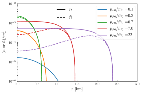
Following the above setup, we first solve the differential equations (60) and (61) with $m_{\phi}=0$ . In Fig. 3, we show the obtained density $n(r)$ and the effective density $\tilde{n}(r)$ profiles for several values of $p_{F0}/\tilde{m}_{0}$ . Recall that the effective density is the number density that includes the suppression factor $\tilde{m}_{\nu}/E_{\mathbf{p}}$ . This factor depends on $p_{F}$ , and decreases toward the center. As a result, suppression in the center is stronger and the maximum of $\tilde{n}(r)$ occurs at certain point away from $r=0$ . This effect becomes stronger with the increase of $p_{F0}/\tilde{m}_{0}$ .

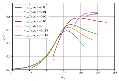
Using the obtained density profiles we computed various characteristics of the neutrino clusters for $y=10^{-7}$ and $m_{\phi}=0$ (see Tab. 1). The correlations of characteristic parameters ( $R$ , $N$ , $p_{F0}$ ) are shown by blue lines in Figs. 4 and 5. For a given value of $p_{F0}/\tilde{m}_{0}$ (second line in Tab. 1) we determined $\tilde{m}_{0}/m_{\nu}$ (the third line). The total numbers of neutrinos $N$ (the first line) was computed according to

N=\int_{0}^{R}n(r)4\pi r^{2}dr.

Using the numbers in the second and third lines we find $p_{F0}/m_{\nu}$ (the 4th line), which in turn, gives the central density of a $\nu$ -cluster:

n_{0}=2.1\cdot 10^{9}\leavevmode\nobreak\ {\rm cm^{-3}}\leavevmode\nobreak\ \left(\frac{p_{F0}}{m_{\nu}}\right)^{3}\left(\frac{m_{\nu}}{0.1\leavevmode\nobreak\ {\rm eV}}\right)^{3}\,.

As $N$ increases, the central density $n_{0}$ (also $p_{F0}$ ) first increases, reaches maximum at $Ny^{3}=1.5\cdot 10^{2}$ or $N=1.5\cdot 10^{23}$ and then it decreases. The maximum corresponds to $p_{F0}\simeq 0.6\leavevmode\nobreak\ m_{\nu}$ , that is, to the point of transition between the non-relativistic and relativistic regimes. The maximal density is determined by the mass of neutrino only:

n_{\nu}^{\max}(0)=4.3\cdot 10^{8}\leavevmode\nobreak\ {\rm cm^{-3}}\left(\frac{m_{\nu}}{0.1{\rm eV}}\right)^{3}.

The corresponding values of radius of a cluster are shown in the last line of Tab. 1. On the contrary, as $N$ increases, the radius $R$ first (in non-relativistic range) decreases, reaches the minimum

R_{\min}\approx 0.62\leavevmode\nobreak\ {\rm km}\left(\frac{10^{-7}}{y}\right)\left(\frac{0.1\ {\rm eV}}{m_{\nu}}\right){\rm km}\thinspace

(64)

at $N\approx 1.5\cdot 10^{23}$ and then increases, as shown in Fig. 4. The minimal radius (64) is about 20% smaller than the non-relativistic result in Eq. (43) for $p_{F}=0.3m_{\nu}$ , which can still be accurately computed using the non-relativistic approximation according to the difference between the dashed and solid curves in Fig. 3.

Notice that dependence $n(r)$ substantially differs from $n(r)=p_{F}^{3}(r)/6\pi^{2}$ with $p_{F}(r)$ taken from the ansatzes of Wise and Zhang (2015). For some distances $r$ , the difference is given by a factor of 5 to 6. At the same time there is good agreement of our $n(r)$ shown in Fig. 3 with that obtained in Gresham et al. (2017).

Table 1: Characteristics of final (degenerate) states of neutrino clusters for

y=10^{-7}

and

m_{\phi}=0

$N$	$2.96\cdot 10^{21}$	$1.63\cdot 10^{22}$	$5.96\cdot 10^{22}$	$9.35\cdot 10^{23}$	$2.34\cdot 10^{24}$
$p_{F0}/\tilde{m}_{0}$	0.10	0.31	0.75	7.0	22
$\tilde{m}_{0}/m_{\nu}$	0.991	0.922	0.688	0.060	0.014
$p_{F0}/m_{\nu}$	0.099	0.286	0.561	0.420	0.308
$n_{0}$ [cm^-3]	$2.0\cdot 10^{6}$	$4.9\cdot 10^{7}$	$3.7\cdot 10^{8}$	$1.5\cdot 10^{8}$	$6.1\cdot 10^{7}$
$R$ [km]	1.25	0.75	0.62	1.46	2.41

The effective neutrino mass at the border of the cluster can be obtained as $\tilde{m}_{\nu}(R)=m_{\nu}+V(R)$ with $V(R)$ defined in Eq. (13):

\tilde{m}_{\nu}(R)=m_{\nu}-\frac{y^{2}}{m_{\phi}R}e^{-m_{\phi}R}\int_{0}^{R}r\tilde{n}(r)\sinh(m_{\phi}r)dr.

Here $\tilde{n}(r)$ should be computed according to Eq. (59). For $m_{\phi}=0$ the expression simplifies to

\tilde{m}_{\nu}(R)=m_{\nu}-\frac{y^{2}}{R}\int_{0}^{R}\tilde{n}(r)r^{2}dr.

Dependence of $N$ and $R$ on $y$ can be obtained using rescaling: $r\to\overline{r}=ry,m_{\phi}\to\overline{m}_{\phi}=m_{\phi}/y$ — see Eq. (151) in Appendix G. The rescaling means that relative effects of the density gradient and mass of $\phi$ in the equation for $\tilde{m}_{\nu}$ do not change with $y$ , if $m_{\phi}/y$ is given at a fixed value. We can write

R(y)=R_{7}\left(\frac{10^{-7}}{y}\right),\leavevmode\nobreak\ \leavevmode\nobreak\ \leavevmode\nobreak\ N(y)=N_{7}\left(\frac{10^{-7}}{y}\right)^{3},

(65)

where $R_{7}$ and $N_{7}$ are the radius and density at $y=10^{-7}$ given in the Table I. From Eq. (65), we find e.g. that at $y=10^{-14}$ and parameters in the last column of the Table I, $R=2.4\cdot 10^{12}$ cm and $N=2.3\cdot 10^{45}$ , which corresponds to $M=3.3\cdot 10^{12}$ g. For $m_{\phi}=0$ , the distribution in $r$ simply dilates with $y$ , and $N$ changes correspondingly.

According to Tab. 2, for small $N$ the field $\phi$ in a cluster is weak, therefore $\tilde{m}_{\nu}\approx m_{\nu}$ and $p_{F0}/\tilde{m}_{0}\approx p_{F0}/m_{\nu}$ . With increase of $N$ the field increases, $\tilde{m}_{0}$ decreases, i.e., the medium suppresses the effective neutrino mass. $N_{7}=1.5\cdot 10^{23}$ is critical value between the non-relativistic and relativistic cases. Further increasing $N$ , the dependence of $R$ and $n_{0}$ on $N$ becomes opposite: $R$ increases, while $n_{0}$ decreases.

V.3 Neutrino clusters for nonzero $m_{\phi}$

The dependence of properties of a $\nu$ -cluster on $m_{\phi}$ is rather complicated. With increase of $m_{\phi}$ the radius of scalar interaction becomes smaller and hence the interactions become weaker. Therefore, in general, one expects that the binding effect weakens and the system becomes less compact for a fixed $N$ . As a result, the radius $R$ increases with increase of $m_{\phi}$ , which indeed is realized in the non-relativistic case.

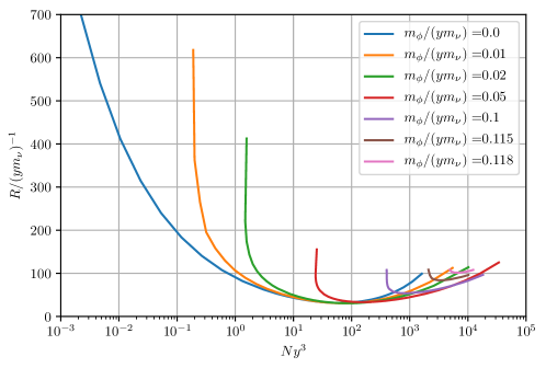
In Fig. 4 we show the dependence of the radius $R$ on $N$ for different values of $m_{\phi}$ . For a given $m_{\phi}$ the dependence has a minimum $R_{\min}$ . As in the massless case, with increase of $N$ the radius first decreases, reaches minimum and then increases in the relativistic regime. This behavior is explained by the fact that in the relativistic case the attractive force is suppressed by $\tilde{m}_{\nu}/E$ , and with increase of $N$ the effective mass $\tilde{m}_{\nu}$ decreases.

The main features of dependence of $R$ on $N$ are discussed below.

(i) Existence of a lower bound on $N$ . At certain $N$ the lines become vertical. The bound is absent for $m_{\phi}=0$ . For each nonzero $m_{\phi}$ , there is a lower bound, $N_{\min}$ , below which it is impossible to make the neutrinos confined. Since the potential energy (attraction) increases with $N$ , to support bound system one should have large enough number of neutrinos. $N_{\min}$ increases with increase of $m_{\phi}$ , that is, with decrease of radius of interactions of individual neutrinos $1/m_{\phi}$ . The smaller the radius, the larger $N$ should be to keep the system bounded.

The dependence of $R$ on $N$ in Fig. 4 differs from that in Fig. 2 of Gresham et al. (2017). In the region of $N$ around minimal radius and above that for $m_{\phi}=0$ radius in Fig. 4 is larger than the radius in Wise and Zhang (2015) and Gresham et al. (2017) and the difference increases with decrease of $N$ . The difference is due to that Gresham et al. (2017) used an analytical solution for $\phi$ which is only valid when $\tilde{n}$ is a constant.

Furthermore, the curves $R=R(N,m_{\phi})$ of Gresham et al. (2017) do not extend far below $N$ that correspods to the minimum of $R$ , since the number $N$ becomes small. Indeed, in Gresham et al. (2017) the constant $\alpha_{\phi}\sim(0.01-0.1)$ corresponds to $y^{3}=(0.045-1.4)$ . For $N\geq 10^{2}$ this gives $Ny^{3}\geq(4.5-140)$ . Our results extend to much smaller values of $Ny^{3}$ , where important feature of existence of minimal value of $N$ for $m_{\phi}\neq 0$ is realized.

The dependence of $R$ on $m_{\phi}$ for fixed $N$ is also similar here to those in Gresham et al. (2017). In the relativistic branch the radius decreases with the increase of $m_{\phi}$ .

For $m_{\phi}=0$ (blue line) the dependence of $R$ on $N$ is well reproduced by Eq. (45) in the non-relativistic case. Notice that in this case the scale of $R$ is related to the neutrino mass.

(ii) Existence of a minimal radius for a given $m_{\phi}$ . The minimum corresponds to $p_{F0}\sim\tilde{m}_{\nu}$ (i.e. to the effective mass of neutrinos which can be much smaller than the vacuum mass). This minimal radius, $R_{\min}$ , in the $m_{\phi}=0$ case is determined by Eq. (64). For nonzero $m_{\phi}$ , it becomes larger because nonzero $m_{\phi}$ suppresses the Yukawa potential exponentially.

With increase of $m_{\phi}$ the minimum $R_{\min}$ shifts to larger $N$ . The value $R_{\min}$ itself changes weakly. For large $m_{\phi}$ the minimum of $R(N)$ does not correspond to $\tilde{m}_{\nu}\sim p_{F0}$ , but still occurs close to transition from NR to UR regimes. Because of the shift of the curves for fixed $N$ in the NR regime the radius increases with increase of $m_{\phi}$ , while in the UR case it decreases. The shift can be interpreted in the following way: For fixed $R$ the volume per neutrino is determined by $m_{\phi}$ : $V_{1}\propto(1/m_{\phi})^{\kappa}$ ( $\kappa\sim 3$ ). Therefore with increase of $m_{\phi}$ , the volume per neutrino decreases and the total number of $N$ in a cluster increases.

There is maximal value of $m_{\phi}$ for which solution with finite radius exists. With approaching of $m_{\phi}$ to this value the curve further shifts to larger $N$ and minimum moves up. For $m_{\phi}>m_{\phi}^{\max}$ the radius of interaction becomes too short to bound the neutrino system and the system disintegrates. The upper bound on $m_{\phi}$ corresponds to the lower bound on strength of interaction:

S_{\phi}\equiv\frac{y^{2}m_{\nu}^{2}}{m_{\phi}^{2}}\gtrsim S_{\phi}^{\min}=70\,,

(66)

which can be compared with the bound $G_{\phi}>3.27$ found in Stephenson et al. (1998) from the condition of existence of minimum of total energy per neutrino for infinite medium. Notice that our bound is obtained from condition of stability of finite configuration.

Let us compare the radius $R$ with the radius of interactions $R_{\phi}=1/m_{\phi}$ . For small $m_{\phi}$ there is the range of values of $N$ in which $R<1/m_{\phi}$ . It is possible to obtain $R=R_{\phi}$ at two different values of $N$ . For $m_{\phi}=0.03ym_{\nu}$ the equality $R=R_{\phi}$ is fulfilled at definite value $N=10^{2}/y^{3}$ . For $m_{\phi}>0.03ym_{\nu}$ , we have $R>R_{\phi}$ for all $N$ and the difference between them increases. $R$ can be orders of magnitude larger than $R_{\phi}$ and therefore in general $1/m_{\phi}$ does not determine the size of the cloud and fragmentation scale.

We denote by $X$ and $Y$ the values at horizontal and vertical axes of Fig. 4 correspondingly:

X\equiv Ny^{3}\leavevmode\nobreak\ \leavevmode\nobreak\ {\rm and}\leavevmode\nobreak\ \leavevmode\nobreak\ \leavevmode\nobreak\ Y\equiv Rym_{\nu}.

The coordinate $Y$ can be written as $Y=R/R_{\phi}S_{\phi}^{-1/2}$ . Therefore the radius of a cluster over the radius of interactions equals

\frac{R}{R_{\phi}}=YS_{\phi}^{-1/2}.

(67)

For $S_{\phi}^{-1/2}=0.01$ the radius (in units $ym_{\nu}$ ) is in the interval $Y=(30-180)$ (see Fig. 4) which gives according to Eq.(67) $R/R_{\phi}=0.3-1.8$ . For $S_{\phi}^{-1/2}=0.02$ the corresponding numbers are $Y=(30-170)$ and $R/R_{\phi}=(0.6-3.4)$ . For $S_{\phi}^{-1/2}=0.1$ we have $Y=(55-110)$ and $R/R_{\phi}=5-11$ . Thus, with decrease of strength the radius increases and becomes substantially larger than $R_{\phi}$ . This regime was observed in Gresham et al. (2017) and called “saturation”. Still $1/m_{\phi}$ determines the scale of sizes of $\nu$ -clusters within an order of magnitude.

In Fig. 5 we show the dependence of $p_{F0}$ (and consequently, the central density) on $N$ for different values of $m_{\phi}$ . For fixed $m_{\phi}$ , $p_{F0}$ as a function of $N$ has a maximum. With increase of $m_{\phi}$ , this maximum shifts to larger $N$ and increases. However, this increase slows down and is restricted by $p_{F0}/m_{\nu}\lesssim 0.9$ . Explicitly, for this value

n_{0}^{\max}=1.5\cdot 10^{9}{\rm cm^{-3}}\left(\frac{m_{\nu}}{0.1{\rm eV}}\right)^{3}.

(68)

With increase of $m_{\phi}$ the central density decreases at small $N$ (the NR regime) and it increases at larger $N$ (UR regime). This anti-correlates with change of radius (for fixed $N$ ) in Fig. 4. The maximal density (corresponding to the maximal $p_{F0}$ ) increases with $m_{\phi}$ and shifts to larger $N$ . The anticorrelation is due to the relation

N\sim b\frac{4\pi}{3}R^{3}n_{F0}=b\frac{2}{9}\pi R^{3}p_{F0}^{3},

(69)

where $b\approx 0.2-0.5$ is smaller than 1, since the density distribution is not uniform and the density is substantially smaller than $n_{F0}$ in peripheral regions.

Thus, the overall change of characteristics of cluster (for fixed $N$ ) with $m_{\phi}$ is the following: In the NR case central density decreases and radius increases (cluster becomes less compact). In the UR case, the radius varies non-monotonically with $m_{\phi}$ , as shown by the relativistic branches of the curves in Fig. 4. These characteristics could be important for cluster formation processes.

For fixed $m_{\phi}$ the bound system exists for $N$ above certain minimal value. With the increase of $N$ the central density (and $p_{F0}$ ) increases quickly and therefore the radius of cluster decreases. Then the density reaches its maximum and with further increase of $N$ the density decreases. Correspondingly the radius of cluster increases.

Notice that strengths of interactions in the case of two neutrino bound states $\lambda$ [see Eq. (19)] and for the bound neutrino system [Eq. (66)] have different functional dependence on the parameters. From Eqs. (19) and (66) we obtain the following relation between the two strengths:

\lambda^{2}=\left(\frac{y}{8\pi}\right)^{2}S_{\phi}.

For $y\leq 10^{-7}$ and $\lambda^{2}\geq 0.7$ required to have $2\nu$ -bound state we find $S_{\phi}>6.3\cdot 10^{16}$ . That is, if $2\nu$ -bound states exist also $\nu$ -clusters should exist. The opposite does not work: For $S_{\phi}\sim 10^{2}$ we have $\lambda\sim 1.6\cdot 10^{-15}$ , and so the $2\nu$ bound states are not possible. Both the bound states and bound systems exist for very small masses of scalars.

V.4 Neutrino bound systems for given $y$ and $m_{\phi}$

In the previous sections we focused on properties of final stable configurations of neutrino clusters. Let us comment on implications of the obtained results.

From the particle physics perspective the input parameters are $y$ and $m_{\phi}$ , and the questions are whether bound systems for given $y$ and $m_{\phi}$ exist, and what the characteristic parameters of these systems are. The parameters $y$ and $m_{\phi}$ determine the interaction strength $S_{\phi}$ defined in Eq. (66). The main condition for existence of bound system is that the strength $S_{\phi}$ is large enough, satisfying the lower bound (66) or $S_{\phi}^{-1/2}\leq 0.12$ . For a given $y$ , the condition on the strength gives an upper bound on $m_{\phi}$ . So, essentially $y$ and $S_{\phi}$ determine all other characteristics.

Let us consider properties of clusters at the critical (minimal) value of strength. According to Fig. 4, $S_{\phi}^{\min}$ is realized at

X^{\rm cr}\approx 10^{4},\,\,\,Y^{\rm cr}\approx 10^{2}

with very small spread. As follows from Fig. 5, it corresponds to maximal $p_{F0}/m_{\nu}=0.86$ and therefore maximal central density of the cluster. With these specific values of $X$ and $Y$ , the parameters of cluster are determined by $y$ . Taking $y=10^{-7}$ , we obtain

m_{\phi}^{\rm cr}\approx 10^{-8}m_{\nu}=10^{-9}\,{\rm eV},

and

N^{\rm cr}=X^{\rm cr}y^{-3}\approx 10^{25},\leavevmode\nobreak\ \leavevmode\nobreak\ \leavevmode\nobreak\ R^{\rm cr}=2\cdot 10^{-4}{\rm cm}\leavevmode\nobreak\ Y^{\rm cr}y^{-1}\approx 2\cdot 10^{5}{\rm cm}.

If $m_{\phi}<m_{\phi}^{\rm cr}$ (for fixed $y$ ), the strength increases and according to Fig. 4, the ranges of $X$ and $Y$ expand. Correspondingly,

N=Xy^{-3}=10^{25}X/X^{\rm cr},

and therefore clusters with much smaller number of neutrinos are possible. E.g. for $S_{\phi}=10^{4}$ , $X$ can be as small as 0.2, and therefore $N=2\cdot 10^{20}$ . $X$ becomes a free parameter in the interval $0.2-10^{4}$ . The allowed range of $Y$ expands in both directions: $Y$ can be as small as $0.3Y^{\rm cr}$ , and therefore the radius reduces down to $0.7$ km. The maximal value of $Y$ can be much bigger than $Y^{\rm cr}$ and it increases with increase of strength (decrease of $m_{\phi}$ ).

R=2\cdot 10^{-4}{\rm cm}\leavevmode\nobreak\ Yy^{-1}=2\cdot 10^{5}{\rm cm}\leavevmode\nobreak\ Y/Y^{\rm cr}.

For $S_{\phi}=10^{4}$ (orange line in Fig. 4) $Y=(30-380)$ and correspondingly, $R=(0.6-7.6)$ km. If also $y$ decreases and $m_{\phi}$ decreases, so that $S_{\phi}$ does not change, the line $Y=Y(X)$ is the same, but parameters of cluster increase as $N\propto y^{-3}$ , $R\propto y^{-1}$ .

For fixed $y$ and $m_{\phi}$ stable bound systems are situated along the corresponding lines $S_{\phi}={\rm const}$ in Figs. 4 and 5. This, in turn, fixes the interval of $X$ and $Y$ (hence $N$ and $R$ ):

N\in\frac{1}{y^{3}}\left[X_{{\rm min}},\,X_{{\rm max}}\right]\thinspace,\,\,\,\,\,R\in\frac{1}{ym_{\nu}}[Y_{{\rm min}},\,Y_{{\rm max}}]\thinspace.

(70)

As an example, for $y=10^{-20}$ and $m_{\phi}=10^{-23}$ eV we obtain $S_{\phi}^{-1/2}=0.01$ (orange line), and according to Fig. 4 we have $X\in[0.2,\ 5\cdot 10^{3}]$ . For chosen $y$ , this gives $N\in[2\cdot 10^{59},\ 5\cdot 10^{63}]$ . Depending on $N$ , the central density changes (see Fig. 5) following the relation (69). The interval $Y\in[30,\ 370]$ (Fig. 4) corresponds to the interval of values $R\in[6\cdot 10^{17},\ 7.4\cdot 10^{19}]$ cm and $R/R_{\phi}\in[0.3,\ 3]$ . With increase of $y$ for fixed strength, $N$ and $R$ change as in Eq. (70). With decrease of strength, the intervals of $X$ and $Y$ shrink. Thus for $S_{\phi}^{-1/2}=0.1$ , we have $X\in[400,\ 2\cdot 10^{4}]$ and $Y\in[50,\ 110]$ . If $y=10^{-20}$ and $m_{\phi}=10^{-22}$ eV, we obtain $N\in[4\cdot 10^{62},\ 2\cdot 10^{64}]$ and $R\in[10^{18},\ 2.3\cdot 10^{18}]$ cm.

From the cosmological perspective the key input parameter is $N$ . It is this quantity that determines in the nearly uniform background evolution and formation of clusters. If $N$ is conserved (no merging of clusters, no particle loss, etc.), this quantity determines the final radius and density of the cluster. From Eq. (45) we obtain

R=1.8\leavevmode\nobreak\ {\rm km}\leavevmode\nobreak\ \left(\frac{10^{-7}}{y}\right)^{2}\left(\frac{10^{21}}{N}\right)^{1/3},

and from Eqs. (44) and (46):

n_{0}=2.25\cdot 10^{8}\leavevmode\nobreak\ {\rm cm^{-3}}(y^{3}N)^{2}.

These relations are valid for $m_{\phi}\ll 1/R$ . With decrease of $y$ (and fixed $N$ ), $R$ increases as $1/y$ and the density decreases as $y^{3/2}$ .

VI Formation of neutrino clusters

Let us consider the formation of neutrino clusters from the uniform background of relic neutrinos in the course of cooling and expansion of the Universe.

We find that for the allowed values of $y$ and $m_{\nu}$ , the typical time of cooling via $\phi$ bremsstrahlung and via annihilation $\nu\bar{\nu}\rightarrow\phi\phi$ are much larger than the age of the Universe (see Appendices I and J). Therefore the formation of neutrino clusters differs from the formation of usual stars.⁵⁵5 Notice that the formation of neutrino clusters is very different from the formation of nuggets of ADM Gresham et al. (2018). The latter proceeds via fusion of particles of DM and requires C-asymmetry to avoid complete annihilation. As we will show in subsections VI.3 and VI.4, for the interaction strength above a certain critical value it has a character of phase transition at which the kinetic energy is transformed into the increase of the effective neutrino mass. The mechanism was first suggested in Stephenson et al. (1998) and here we explore it further.

The phase transition leads to fragmentation of the cosmic neutrino background. Here we present some simplified arguments and analytic estimations. A complete solution of the formation problem would require numerical simulation of evolution of the $\nu$ background. Such a simulation is beyond the scope of this paper.

VI.1 Maximal density and fragmentation of the $\nu$ background

The key parameter that determines formation of $\nu$ -clusters is the central density given by Eq. (68). According to Fig. 5, there is a maximal value of $p_{F0}$ , and consequently, a maximal value of the density $n_{0}^{\rm max}$ which is determined by the mass of neutrino in Eq. (68). After the fragmentation of a uniform relic $\nu$ -background (see below), the central density of a cluster stopped decreasing. Consequently, at the epoch of fragmentation the density was

n_{\rm frag}\leq n_{0}^{\max}.

Thus, we can take

n_{\rm frag}\leq 10^{9}\leavevmode\nobreak\ {\rm cm^{-3}}.

In turn, this density determines the epoch of fragmentation:

(z_{f}+1)=\left(\frac{n_{\rm frag}}{n_{\rm rel}}\right)^{1/3}=215,

(71)

where $n_{\rm rel}=113$ is the number density of one neutrino mass state that would be in the present epoch in the absence of clustering. That is, formation of $\nu$ -clusters starts after the epoch of recombination ( $z=1100$ , $T=0.1$ eV). At this epoch ( $z_{f}+1=215$ ) the neutrino average momentum was $p\sim 0.02$ eV. So, fragmentation could start when $p\sim m_{\nu}$ , which is not accidental since $n_{0}^{\max}$ is determined by $m_{\nu}$ only.

VI.2 Evolution of the effective neutrino mass

Dependence of the effective mass $\tilde{m}_{\nu}$ on $T$ plays crucial role in the formation of neutrino bound systems. If neutrinos are the only source of the field $\phi$ , for the allowed coupling constant $\phi$ cannot be thermalized in the early Universe and the amount of $\phi$ particles is negligible. Evolution of the scalar field in expanding universe is described by Eq. (8) with an additional expansion term $3H(t)d\phi/dt$ , where the Hubble constant depends on time as $H(t)=1/2t$ in the radiation-dominated epoch and as $H(t)=2/3t$ in the matter-dominated epoch.

Notice that in general $m_{\phi}\neq 0$ regularizes the procedure of computations. Otherwise, it is regularized by the Hubble expansion rate $H$ . Indeed, from the equation of motion (8) for uniform distribution, assuming $\dot{\phi}=aH\phi$ , where $a$ is the scale factor in the Friedmann-Robertson-Walker (FRW) metric, we obtain

\phi=-\frac{y}{a^{2}H^{2}+m_{\phi}^{2}}\langle\bar{\nu}\nu\rangle,

(72)

and $\langle\bar{\nu}\nu\rangle$ is given in (10). Thus, the expansion term regularizes the solution for $m_{\phi}\rightarrow 0$ . The energy density in the field:

\rho_{\phi}=\frac{y^{2}}{2}\frac{m_{\phi}^{2}}{(a^{2}H^{2}+m_{\phi}^{2})^{2}}|\langle\bar{\nu}\nu\rangle|^{2}.

(73)

In what follows we assume that $H\ll m_{\phi}$ , so that expansion can be treated as slow change of density and temperature in the solution of equation without expansion.

Neglecting the Hubble expansion term, Eq. (72) gives for uniform medium

\phi=-\frac{y}{m_{\phi}^{2}}\langle\bar{\nu}\nu\rangle.

(74)

From Eq. (74), we obtain the equation for the effective mass of neutrino:

\tilde{m}_{\nu}=m_{\nu}-\frac{y^{2}}{m_{\phi}^{2}}\langle\bar{\nu}\nu\rangle,

where [see Eq. (10)]

\langle\bar{\nu}\nu\rangle=\frac{\tilde{m}_{\nu}}{2\pi^{2}}\int_{0}^{\infty}\frac{dp\leavevmode\nobreak\ p^{2}}{\sqrt{p^{2}+\tilde{m}_{\nu}^{2}}}f(p,T),

and $f(p,T)$ is the distribution of neutrinos (thermal or degenerate⁶⁶6Notice that results for the degenerate case can be obtained by substituting $I_{3}T^{3}\rightarrow\frac{p_{F}^{3}}{3}$ in the results for the thermal case.). Explicitly the equation for $\tilde{m}_{\nu}$ can be written as

\tilde{m}_{\nu}=m_{\nu}-\frac{y^{2}}{m_{\phi}^{2}}\frac{\tilde{m}_{\nu}}{2\pi^{2}}\int_{0}^{\infty}\frac{dp\leavevmode\nobreak\ p^{2}}{\sqrt{p^{2}+\tilde{m}_{\nu}^{2}}}f(p,T).

Here we use the thermal distribution with $T\neq 0$ , which is relevant for $T>m_{\nu}$ , while in Stephenson et al. (1998) the distribution of degenerate Fermi gas was used. Qualitatively, the results are similar.

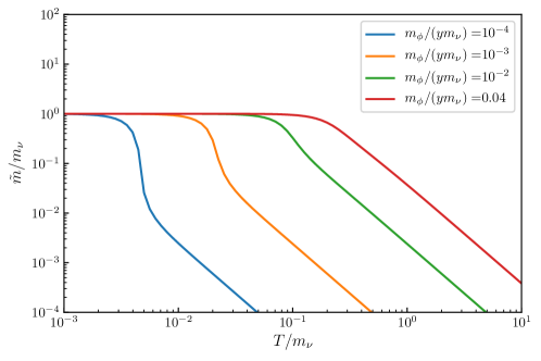
In Fig. 6, we show dependence of $\tilde{m}_{\nu}$ on $T$ for different values of strength of interaction. In the ultra-relativistic limit, $T\gg\tilde{m}$ , we obtain

\tilde{m}_{\nu}=m_{\nu}-\frac{y^{2}\tilde{m}_{\nu}T^{2}}{m_{\phi}^{2}}\frac{I_{2}}{2\pi^{2}},

(75)

where in general, the integrals $I_{n}$ have been introduced in Eq. (48). From Eq. (75) we find

\tilde{m}_{\nu}=\frac{m_{\nu}}{1+\frac{y^{2}T^{2}I_{2}}{2\pi^{2}m_{\phi}^{2}}}\approx m_{\nu}\frac{2\pi^{2}m_{\phi}^{2}}{y^{2}T^{2}I_{2}}=m_{\nu}\frac{24m_{\phi}^{2}}{y^{2}T^{2}}=m_{\nu}\frac{24}{S_{\phi}}\left(\frac{m_{\nu}}{T}\right)^{2}\equiv\tilde{m}_{\nu}^{\rm rel}.

(76)

That is, the effective mass $\tilde{m}_{\nu}\propto T^{-2}$ decreases as $T$ increases and becomes negligible in the early Universe.

In the non-relativistic case, $T\ll\tilde{m}_{\nu}$ , the solutions is

\tilde{m}_{\nu}=m_{\nu}-\frac{y^{2}T^{3}}{m_{\phi}^{2}}\frac{I_{3}}{2\pi^{2}}\equiv\tilde{m}_{\nu}^{\rm nr}.

(77)

That is, as $T\to 0$ , $\tilde{m}_{\nu}\rightarrow m_{\nu}$ . These analytic results agree well with results of numerical computations shown in Fig. 6.

Note that the relativistic regime is determined by $\tilde{m}_{\nu}$ and not $m_{\nu}$ : $T>\tilde{m}_{\nu}$ . The effective mass $\tilde{m}_{\nu}$ increases as $1/T^{2}$ till $T\approx\tilde{m}_{\nu}$ . According to Eq. (76) this equality gives

\frac{T_{\rm rel}}{m_{\nu}}=\left(\frac{24}{S_{\phi}}\right)^{1/3}.

(78)

Below this temperature the growth of $\tilde{m}$ is first faster and then slower than $1/T^{2}$ . The change of derivative occurs at maximum of the relative energy in the scalar field (see below). $\tilde{m}(T)$ converges to the non-relativistic regime at $\tilde{m}_{\nu}^{\rm rel}(T)=m_{\nu}$ . This gives, according to Eq. (76),

\frac{T_{\rm nr}}{m_{\nu}}=\left(\frac{24}{S_{\phi}}\right)^{1/2}.

VI.3 Energy of the $\nu$ - $\phi$ system and the dip

Let us compute the energy density in the scalar field, $\rho_{\phi}$ , in neutrinos, $\rho_{\nu}$ , and the total energy density defined as

\rho_{\rm tot}=\rho_{\nu}+\rho_{\phi}

(79)

as a function of $T$ . Expansion of the Universe can be accounted for by considering the average energy per neutrino:

\epsilon_{i}\equiv\frac{\rho_{i}}{n_{\nu}},\leavevmode\nobreak\ \leavevmode\nobreak\ \leavevmode\nobreak\ \leavevmode\nobreak\ i=\{\nu,\leavevmode\nobreak\ \leavevmode\nobreak\ \phi,\leavevmode\nobreak\ \leavevmode\nobreak\ {\rm tot}\},

(80)

where the number density of neutrinos equals

n_{\nu}=\frac{1}{2\pi^{2}}\int_{0}^{\infty}dp\leavevmode\nobreak\ p^{2}f(p,T)=\frac{I_{3}}{2\pi^{2}}T^{3}.

The energy density in the scalar field is given by

\rho_{\phi}=\frac{1}{2}m_{\phi}^{2}\phi^{2}.

(81)

Here $\phi$ can be expressed via the effective mass, $\phi=(\tilde{m}_{\nu}-m_{\nu})/y$ , and therefore

\rho_{\phi}(\tilde{m}_{\nu})=\frac{m_{\phi}^{2}}{2y^{2}}(\tilde{m}_{\nu}-m_{\nu})^{2}.

(82)

So, $\rho_{\phi}$ is directly determined by the deviation of the effective mass of neutrino from the vacuum mass. The energy per neutrino equals

\epsilon_{\phi}=m_{\nu}\frac{\pi^{2}}{I_{3}S_{\phi}}\left(\frac{\tilde{m}_{\nu}}{m_{\nu}}-1\right)^{2}\left(\frac{m_{\nu}}{T}\right)^{3}.

(83)

Using the known form of $\tilde{m}_{\nu}(T)$ , Eq. (75), we compute the energy density $\epsilon_{\phi}$ . In the ultra-relativistic limit, according to Eq. (82), the energy density in $\phi$ converges to the constant:

\rho_{\phi}^{\rm rel}=\frac{m_{\phi}^{2}}{2y^{2}}m_{\nu}^{2}.

Therefore

\epsilon_{\phi}^{\rm rel}=\frac{m_{\nu}}{\chi},

where

\chi\equiv\frac{S_{\phi}I_{3}}{\pi^{2}}\left(\frac{T}{m_{\nu}}\right)^{3}.

In the non-relativistic limit

\rho_{\phi}^{\rm nr}=\frac{1}{8\pi^{4}}\frac{y^{2}}{m_{\phi}^{2}}I_{3}^{2}T^{6}.

and

\epsilon_{\phi}^{\rm nr}=m_{\nu}\frac{S_{\phi}I_{3}}{4\pi^{2}}\left(\frac{T}{m_{\nu}}\right)^{3}=\frac{m_{\nu}}{4}\chi.

(84)

According to Eq. (84), as the Universe cools down, $\epsilon_{\phi}$ first increases and then decreases. The maximum of $\epsilon_{\phi}$ is achieved when $\epsilon_{\phi}^{\rm rel}\approx\epsilon_{\phi}^{\rm nr}$ , which happens at $\chi=2$ , or

\frac{T^{\max}}{m_{\nu}}=\left(\frac{2\pi^{2}}{S_{\phi}I_{3}}\right)^{1/3}.

Hence the maximum is $\epsilon^{\max}=m_{\nu}/2$ . When $S_{\phi}$ increases (correspondingly $m_{\phi}$ decreases), the maximum $\epsilon^{\max}$ does not change significantly, but shifts to smaller $T$ .

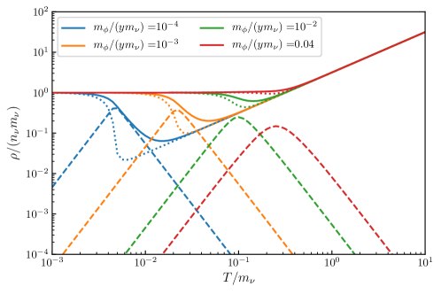
In Fig. 7, we show the dependence of $\epsilon_{\phi}/m_{\nu}$ on $T$ (dashed lines). As can be easily checked, the analytic expressions above agrees well with the numerical results.

The energy density of neutrinos is given by

\rho_{\nu}(\tilde{m}_{\nu})=\frac{1}{2\pi^{2}}\int_{0}^{\infty}dp\leavevmode\nobreak\ p^{2}\sqrt{p^{2}+\tilde{m}_{\nu}^{2}}f(p,T).

It can be rewritten as

\rho_{\nu}(\tilde{m}_{\nu})=\frac{1}{2\pi^{2}}\left[\int_{0}^{\infty}\frac{dp\leavevmode\nobreak\ p^{4}}{\sqrt{p^{2}+\tilde{m}_{\nu}^{2}}}f(p,T)+\tilde{m}_{\nu}^{2}\int_{0}^{\infty}\frac{dp\leavevmode\nobreak\ p^{2}}{\sqrt{p^{2}+\tilde{m}_{\nu}^{2}}}f(p,T)\right].

(85)

Here the second integral coincides with integral in $\langle\bar{\nu}\nu\rangle$ and $\phi$ . The dependence of $\rho_{\nu}(\tilde{m}_{\nu})$ on $T$ can be found explicitly.

In the non-relativistic case we obtain from Eq. (85)

\rho_{\nu}^{\rm nr}=\frac{1}{2\pi^{2}}\left[\tilde{m}_{\nu}I_{3}T^{3}+\frac{1}{\tilde{m}_{\nu}}I_{5}T^{5}\right]\approx\frac{1}{2\pi^{2}}m_{\nu}I_{3}T^{3},

and consequently, $\rho_{\nu}^{\rm nr}=m_{\nu}n_{\nu}$ , or

\epsilon_{\nu}^{\rm nr}=m_{\nu}.

In the relativistic case, we have

\rho_{\nu}^{\rm rel}=\frac{1}{2\pi^{2}}\left[I_{4}T^{4}+\tilde{m}_{\nu}^{2}I_{2}T^{2}\right]\approx\frac{I_{4}}{2\pi^{2}}T^{4}\approx\frac{7\pi^{2}}{240}T^{4},

and

\epsilon_{\nu}^{\rm rel}=\frac{I_{4}}{I_{3}}T\approx 3.15T,

as expected. The dependence of $\epsilon_{\nu}$ on $T$ is shown in Fig. 7 (dotted lines).

Solid lines in Fig. 7 correspond to the total energy (80). Scalar contributions shift the minimum of $\epsilon_{\rm tot}$ to slightly larger $T$ with respect to the minimum of $\epsilon_{\nu}$ .

The key feature of the $\epsilon_{\rm tot}$ dependence on $T$ is development of the dip at some temperature below $m_{\nu}$ , denoted by $T_{\rm dip}$ .

According to Fig. 7, $\epsilon_{\rm tot}$ becomes smaller than $m_{\nu}$ when $T\simeq m_{\nu}/3$ . As $T$ decreases below $T_{\rm dip}$ , the energy $\epsilon_{\rm tot}$ converges to $m_{\nu}$ from below. The dip essentially coincides with the transition region for $\tilde{m}_{\nu}$ (Fig. 6).

Without the Yukawa interaction (or if the Yukawa interaction is too weak, as illustrated by the red line for $S_{\phi}=0.04^{-2}=625$ in Fig. 7), $\epsilon_{\rm tot}$ would decrease as $\epsilon_{\rm tot}\propto T$ in the relativistic case; at $T\simeq m_{\nu}/3$ , the curve flattens and $\epsilon_{\rm tot}$ converges to $m_{\nu}$ . For the entire range it would always be $\epsilon_{\rm tot}>m_{\nu}$ which corresponds to unbounded neutrinos. For larger $S_{\phi}$ (other curves in Fig. 7), the dip appears. The appearance of the dip with $\epsilon_{\rm tot}<m_{\nu}$ means that neutrinos can form bound systems with the average binding energy equal to $m_{\nu}-\epsilon_{\rm tot}$ . As the interaction strength increases, the dip shifts to lower temperatures and becomes deeper. Correspondingly the binding energy becomes stronger.

The critical value of the strength needed for existence of the dip, $S_{\phi}^{c}$ , is determined by the condition that temperature of beginning of deviation of $\epsilon_{\nu}^{\rm rel}$ from linear decrease equals $T_{\rm rel}\approx m_{\nu}/3$ . This temperature coincides with $T_{\rm rel}$ of deviation of $\tilde{m}_{\nu}$ from its $1/T^{2}$ behavior. The condition (78) can be rewritten as

S_{\phi}^{c}\approx 24\left(\frac{m_{\nu}}{T_{\rm rel}}\right)^{3}.

Then for $T_{\rm rel}/m_{\nu}\approx 1/3$ it gives $S_{\phi}^{c}=580$ , which is close to $S_{\phi}=625$ for the red curve in Fig. 7. In actual numerical calculations, we find that the dip appears roughly at $S_{\phi}^{c}\approx 700$ .

VI.4 Fragmentation

Here we consider $S_{\phi}>S_{\phi}^{c}$ so that the dip occurs. Above $T_{\rm dip}$ , cosmic neutrinos evolve as a uniform background with decreasing density and effective temperature. For $T<T_{\rm dip}$ , further cosmological expansion assuming the uniform neutrino background would imply that the energy of the system increases. Since there is no injection of energy into the $\nu$ - $\phi$ system from outside, it is energetically profitable that the uniform neutrino background fragments into parts (clusters) with the temperature $T\approx T_{\rm dip}$ , which determines also the corresponding number density. Further evolution of fragments will proceed, subject to the dynamics of $\nu$ clusters. The expansion of the Universe then increases the distance between fragments.

The highest temperature of fragmentation corresponds to $T_{f}\sim 0.3m_{\nu}\sim 0.03$ eV. This temperature is achieved at redshift $z_{f}=200$ when the number density of neutrinos was

n_{f}=9\cdot 10^{8}\,\,{\rm cm}^{-3}.

(86)

In the process of formation of final configuration this density could further increase in the central parts of objects. This value agrees well with the one in Sec. VI.1.

The biggest possible object after fragmentation, which satisfies minimal (free) energy condition, would have the size $D_{0}\leq 1/2D_{U}(z_{f})$ in one dimension, where $D_{U}(z_{f})$ is the size of horizon in the epoch of fragmentation, $D_{U}(0)=4.2$ Gpc. Therefore in three dimensions one would expect that $2^{3}=8$ such objects could be formed, and for estimations we will use $\sim 10$ objects. At $z_{f}=200$ we find $D_{0}=10$ Mpc. In the present epoch distance between the objects is $z_{f}$ times larger, that is $\sim 2000$ Mpc.

Using the number density density (86) and the radius $R_{f}=5$ Mpc we obtain the total number of neutrinos in a cluster

N_{f}=\frac{4\pi}{3}R_{f}^{3}n_{f}=1.2\cdot 10^{85}.

(87)

Correspondingly, the mass is $M=4\cdot 10^{17}M_{\odot}$ . These biggest structures can be realized for $m_{\phi}=4\cdot 10^{-30}{\rm eV}$ and $y=4\cdot 10^{-27}$ .

If $m_{\phi}$ and $y$ are much larger, these structures do not satisfy conditions for stable bound systems. The number of neutrinos and radii should be much smaller. One can explore two possible ways of formation of small scale structures:

1. The neutrino background first fragments into the biggest structures, thus satisfying the energy requirement. These structures are unstable and further fragment into smaller parts. The secondary fragmentation can be triggered by density fluctuation of the neutrino background itself or via gravitational interactions with already existing structures like the Dark Matter halos.

If the secondary fragmentation is slow, the overall final structure could consist of superclusters (originated from primary fragmentation) and clusters within superclusters.

2. The uniform neutrino background may immediately fragment into small structures (close to final stable bound states) with $R={\cal O}(1/m_{\phi})$ . These structures may interact among themselves.

As we established, for given $m_{\phi}$ and $y$ (i.e. fixed strength) there is a range of stable configurations with different $N$ and $R$ . E.g. for $S_{\phi}^{-1/2}=0.01$ , $N$ can be within 4 orders of magnitude. What is the distribution of clusters with respect to $N$ ? The answer depends on details of formation, in particular, on the surface effects. One can consider several options:

(i) a flat distribution within the allowed interval;

(ii) a peak at $N=X(n_{F0})/y^{3}$ , where $n_{F0}$ is the density at the beginning of fragmentation which, in turn, is determined by the strength, etc.

Considering $T_{\min}$ as the temperature of the beginning of fragmentation we can find using Figs. 6 and 7 the physical conditions of medium which determine the initial states of pre-clusters. The kinetic energy per neutrino is (in the unit of $m_{\nu}$ ) $\epsilon^{\rm kin}=3.14T_{\min}/m_{\nu}$ . The kinetic energy turns out to be much bigger than $\tilde{m}(T_{\min})$ :

\epsilon^{\rm kin}\gg\tilde{m}(T_{\min}).

So neutrinos are ultra-relativistic and therefore our usage of the relativistic distribution is justified. Correspondingly, the total energy in neutrinos nearly coincides with the kinetic energy: $\epsilon_{\nu}\approx\epsilon^{\rm kin}$ .

Thus, for $S_{\phi}^{-1/2}=10^{-3}$ we obtain from Figs. 6 and 7: $T_{\min}/m_{\nu}=5\cdot 10^{-2}$ , $\epsilon^{\rm kin}=0.15$ , and $\tilde{m}/m_{\nu}=0.01$ . The energy in the scalar field is substantially smaller than in neutrinos: $\epsilon_{\phi}=0.05$ . However it increases quickly with the temperature further decreasing. The total energy in the system is $\epsilon_{\rm tot}=0.2$ .

The number density of neutrinos is given by $n_{0}^{\min}=2\cdot 10^{6}$ cm^-3 which would correspond to the Fermi momentum $p_{F}/m_{\nu}=0.1$ . This momentum is smaller than the kinetic energy, so the cooling is needed to reach degenerate configuration.

Further results and statements should be considered as a possible trend since to construct the figures we used approximation of uniform infinite medium and relativistic distributions of neutrinos over momenta. Below $T_{\rm dip}$ , the dynamics of finite size objects should be included.

As $T$ deceases below $T_{\min}$ , the kinetic energy of neutrinos decreases while the effective mass $\tilde{m}$ increases. This means that the kinetic energy transforms into the increase of the mass as well as into the energy of scalar field. Thus, for $T/m_{\nu}=0.03$ we obtain $\epsilon^{\rm kin}=0.09$ , $\tilde{m}/m_{\nu}=0.03$ , i.e. the ratio $\epsilon^{\rm kin}m_{\nu}/\tilde{m}=3$ ; for $T/m_{\nu}=0.02$ the ratio becomes 0.3.

According to Figs. 6 and 7, the minimum of total neutrino energy, $\epsilon_{\nu}$ , is achieved at a temperature lower than $T_{\rm dip}$ . In the minimum, for $S_{\phi}^{-1/2}=10^{-3}$ , $\epsilon_{\nu}=0.1$ and $\tilde{m}/m_{\nu}=0.07$ , i.e. neutrinos become non-relativistic.

As $T$ further decreases, both $\epsilon_{\nu}$ and $\tilde{m}$ quickly increase with $\tilde{m}\rightarrow\epsilon_{\nu}$ . This indicates that the kinetic energy is transformed into $\tilde{m}$ as well as into $\epsilon_{\phi}$ . One can guess that the phase transition ends when $\epsilon_{\phi}$ reaches maximum which corresponds to the maximal potential energy. This happens at a slightly lower temperature than the temperature of $\epsilon_{\nu}$ reaching its minimum.

The period of (primary) fragmentation can be estimated as the time interval which corresponds to the width of the dip:

\Delta t=t(T_{1})-t(T_{2}),

(88)

where $t\approx\frac{2}{3H(T)}$ (for matter dominated era) and $H$ is roughly proportional to $T^{2}$ . The specific form can be determined by $H^{2}=8\pi\rho_{{\rm total}}/(3m_{{\rm pl}}^{2})$ where $\rho_{{\rm total}}$ is the total energy density of the Universe and $m_{{\rm pl}}$ is the Planck mass. The two temperatures $T_{1}$ and $T_{2}$ correspond to the maximum of the dashed curve in Fig. 7 and the minimum of the solid curve respectively. This gives e.g. $\Delta t=0.014\tau_{U}$ for $S_{\phi}^{-1/2}=10^{-3}$ and $\Delta t=0.24\tau_{U}$ for $S_{\phi}^{-1/2}=10^{-4}$ , where $\tau_{U}$ is the present age of the Universe. Note that the estimations based on Fig. 7 may not be reliable since in the region of temperatures below $T_{\rm dip}$ neutrinos become non-relativistic and the dynamics of clusters starts to dominate.

According fo Fig. 7, $T_{\rm dip}$ decreases as $S_{\phi}$ increases. This means that for larger $S_{\phi}$ , fragmentation starts at later epochs and lower densities. For $S_{\phi}^{-1/2}=(0.12,\leavevmode\nobreak\ 10^{-2},\leavevmode\nobreak\ 10^{-3})$ , we find $T_{\rm min}/m_{\nu}=(0.3,\leavevmode\nobreak\ 0.12,\leavevmode\nobreak\ 0.04)$ , $n_{0}=(9\cdot 10^{8},\leavevmode\nobreak\ 5.7\cdot 10^{7},\leavevmode\nobreak\ 2.1\cdot 10^{6})$ cm^-3 and the redshift at fragmentation $(z_{f}+1)=(200,\leavevmode\nobreak\ 80,\leavevmode\nobreak\ 27)$ . With the increase of strength, $n_{0}$ and $p_{F0}$ decrease. Then according to Figs. 5 and 4, $N$ and $R$ decrease.

Let us underline that results on the very fact of formation based on the energy consideration and properties of final configurations are robust. Details and features of fragmentation (the way of fragmentation, the distribution of clusters as a function of $N$ , the level of degeneracy in the final states of bound systems) require further studies, and in general, extensive numerical simulations.

VI.5 Virialization

In the range of $S_{\phi}=70-700$ , the dip disappears and the phase transition is absent. Such interaction strengths still allow for stable bound systems of neutrinos. In this case, $\nu$ clusters might be formed from the growth of local over-density to the non-linear regime and then go also through virialization, similar to the formation of dark matter halos.

Quantitatively, results for Yukawa forces (if $m_{\phi}$ is sufficiently small) can be obtained from the gravitational results by replacing

\frac{GM^{2}}{r}\rightarrow\frac{(yN)^{2}}{4\pi r}\thinspace,

(89)

where $G$ is the gravitational constant and $M=m_{\nu}N$ is the total mass. The key difference from the gravitational case is that the strength of Yukawa interaction is many orders of magnitude larger than the strength of gravity.

With this analogy we can consider the following picture of structure formation.

1. The initial state is the neutrino background with some primordial or initial density perturbations (primordial clouds) with $\Delta n_{p}/n_{p}\ll 1$ and sizes $R_{p}$ . These perturbations may be related to the density perturbation of DM in the Universe, since neutrino structures are formed latter.

2. As the Universe expands, the size of clouds and distance between them increase simultaneously as the scale factor $R\propto d\propto a$ . Correspondingly, the density decreases as $a^{-3}$ and $\Delta n/n$ is constant. This is the linear regime.

3. At certain epoch, when $T<0.3m_{\nu}$ the evolution becomes non-linear: the attraction becomes more efficient than expansion and the increase of the size of clouds becomes slower than the expansion of the Universe. This happens provided that the potential energy of the cloud is substantially larger than the total kinetic energy. Then the distance between two clouds increases faster that size of clouds. Also the decrease of the density slows down. 4. At some point (for which we denote the scale factor by $a_{\max}$ ) the density stops decreasing, and after that ( $a>a_{\max}$ ), the system starts collapsing. In this way a bound system is formed and its evolution is largely determined by internal factors. The distance between two clouds continues increasing.

Since the system is collisionless and there is no energy loss (emission of particles or and waves) the contraction has a character of virialization⁷⁷7A system of collisionless (i.e. no additional interactions except for gravity) particles can collapse from a large cold distribution (or more strictly, a distribution with low mean kinetic energy since it is usually not a thermal distribution) to a smaller and hotter one. This processes is known as virialization., which starts from the stage that kinetic energy of the neutrino system becomes significantly smaller than the potential energy:

\frac{E_{K}}{|E_{V}|}\equiv\xi_{E}\ll 1.

(90)

During virialization, the kinetic energy increases (the effective $T$ increases, although the distribution may not be thermal). The process stops at $a=a_{\rm vir}$ when virial equilibrium is achieved, which also corresponds to hydrostatic equilibrium. The radius decreases by a factor of 2 so that the density increases by a factor of 8. Approaching the equilibrium the cluster may oscillate. At this point, the formation of the cluster is accomplished.

In what follows we will make some estimations and check how this picture matches the final configurations of clusters we obtained before. We will discuss bounds on initial parameters of the perturbations , formation procedure, epochs of different phases, etc, which follow from this matching.

The total energy is conserved during virialization. When the system reaches virial equilibrium, the virial theorem implies that

2E_{K}^{\rm vir}+E_{V}^{\rm vir}=0\leavevmode\nobreak\ \leavevmode\nobreak\ \leavevmode\nobreak\ {\rm or}\leavevmode\nobreak\ \leavevmode\nobreak\ \leavevmode\nobreak\ \frac{E_{K}^{\rm vir}}{E_{V}^{\rm vir}}=\frac{1}{2}\thinspace,

(91)

Here $E_{K}^{\rm vir}$ and $E_{V}^{\rm vir}$ are the total kinetic and potential energies after virialization. Thus, the ratio of energies increases.

Although quantitative studies of virialization involve $N$ -body simulation, the orders of magnitude of various characteristics can be obtained from simplified considerations. For gravitational virialization, it is known that⁸⁸8See, e.g., http://www.astro.yale.edu/vdbosch/astro610_lecture8.pdf or Ref. Mota and van de Bruck (2004). the virialization time (roughly the time of collapse) driven by gravity equals

t_{{\rm vir}}\simeq 2\pi GM\left|\frac{M}{2(E_{K}+E_{V})}\right|^{3/2},

(92)

where $E_{K}$ and $E_{V}$ are the total kinetic and potential energies ( $E_{K}+E_{V}<0$ ) of the system.

The time of $m_{\phi}$ -driven virialization can be obtained from Eq. (92) by making the replacement (89):

t_{{\rm vir}}\simeq\frac{\sqrt{m_{\nu}}N^{5/2}y^{2}}{4\sqrt{2}|E_{K}+E_{V}|^{3/2}}\thinspace.

(93)

The contraction stops when virial equilibrium is achieved and we assume that the equilibrium has the same form as in the gravity case (91). Since the total energy is conserved during virialization,

E_{K}^{{\rm vir}}+E_{V}^{{\rm vir}}=E_{K}+E_{V}\thinspace,

we obtain $E_{K}^{\rm vir}=|E_{K}+E_{V}|$ and $E_{V}^{\rm vir}=-2|E_{K}+E_{V}|$ .

The total energy in the beginning of virialization can be written as

|E_{K}+E_{V}|=|E_{V}|(1-\xi_{E})=\frac{2}{3}|E_{V}|,

where in the last equality we have taken $\xi_{E}=1/3$ . Inserting this total energy with $|E_{V}|$ given in (52) into Eq. (93), we obtain the time of virialization

t_{{\rm vir}}\simeq\sqrt{3}\left(\frac{5}{2}\right)^{3/2}\frac{\pi^{2}}{I_{3}^{1/2}}\frac{1}{ym_{\nu}}\left(\frac{m_{\nu}}{T}\right)^{3/2},

which does not depend on $N$ . Numerically, we get

t_{{\rm vir}}\simeq 3.4\cdot 10^{-6}{\rm sec}\left(\frac{10^{-7}}{y}\right)\left(\frac{0.1{\rm eV}}{m_{\nu}}\right)\left(\frac{m_{\nu}}{T}\right)^{3/2},

(94)

which implies that for $T/m_{\nu}=1$ , the virialization takes $t_{{\rm vir}}\simeq 3.4\cdot 10^{-6}$ sec.

As aforementioned, after the virialization process, the radius decreases by a factor of 2 and correspondingly, the density increases by a factor of 8. Hence in the example we discussed at the end of the previous subsection, this gives $R_{\rm vir}=1.3$ km, and $n_{\rm vir}=7\cdot 10^{10}$ cm^-3.

As a result of virialization, the distribution reaches virial equilibrium with the virialized energies given by

E_{K}^{({\rm vir})}=-\frac{1}{2}E_{V}^{({\rm vir})}=E_{K}^{\rm in}+E_{V}^{\rm in}.

(95)

A halo of neutrinos is formed. In the absence of energy loss, its number density remains constant without being diluted by $a^{-3}$ ( $a$ is the scale factor) due to the cosmological expansion. That is, a halo of high-density cosmic neutrinos would be frozen till today.

Let us estimate temperatures of the $\nu$ -clusters at different phases of formation. We can assume that deviation from the linear regime occurs at $T\sim m_{\nu}$ . Also we assume that before collapse the state of the system can be approximately described by thermal equilibrium and the border effects can be neglected. Therefore, we can use results obtained in sect. IV C. The expression for temperature (54) can be rewritten as

\frac{T}{m_{\nu}}=5.3\cdot 10^{-3}(y^{3}N)^{2/3}\xi_{E}.

Let us take $y^{3}N=1$ (see implications in the Fig. 4, 5) then $T/m_{\nu}=1$ (the scale factor $a_{NL}$ ) corresponds to $\xi_{E}=189$ . For $\xi_{E}=1/3$ we obtain $T/m_{\nu}=1.8\cdot 10^{-3}$ . For $y^{3}N=32$ , $T/m_{\nu}=1$ corresponds to $\xi_{E}=19$ and $\xi_{E}=1/3$ is achieved at $T/m_{\nu}=1.8\cdot 10^{-2}$ . If $y^{3}N=10^{3}$ , $T/m_{\nu}=1$ is realized at $\xi_{E}=1.9$ , and $\xi_{E}=1/3$ at $T/m_{\nu}=0.18$ .

VI.6 Neutrino structure of the Universe

The formation of the neutrino clusters leads to neutrino structure in the Universe with overdense areas and voids. For simplicity we consider that all the clouds have the same number of neutrinos $N$ .

In the present epoch the distance between neutrinos without clustering equals

d_{0}=(n_{\nu}^{0})^{1/3}=0.2\leavevmode\nobreak\ {\rm cm}.

If neutrinos cluster into clouds with $N$ neutrino in each, the distance between (centers of) these clusters is

d=d_{0}N^{1/3}.

Taking, e.g., $N=6\cdot 10^{22}$ , we obtain $d=78$ km which is much larger than the radius of each cloud, $R=0.62$ km given by Eq. (64).

The existence of such a structure could have an impact on the direct detection of relic neutrinos in future experiments such as the PTOLEMY Baracchini et al. (2018); Betti et al. (2019). The result also depends on the motion of the clusters with respect to the Earth. The motion of the Earth and the solar system will average the effect of these small structures. According to Eq. (45), in the non-relativistic regime the radius of cluster decreases with increase of $N$ as $N^{-1/3}$ . Therefore the ratio of spacing (distance) and radius increases as $\propto N^{2/3}$ :

\frac{d}{R}\approx 1.1\cdot 10^{-2}\leavevmode\nobreak\ d_{0}m_{\nu}y^{2}N^{2/3}.

Taking the above example ( $d=78$ km, $R=0.62$ km), we have $d/R=126$ . So, voids occupy most of the space. With decrease of $y$ , the radius of cluster increases and $N$ also increases (for fixed maximal density). As a result, $d/R=$ const which is determined by the neutrino mass.

Let us estimate how small scale clusters may affect the direct detection of relic neutrinos assuming that clouds reached their final configurations. The distance needed for a detector to travel through to meet a $\nu$ -cluster, in average, can be estimated as $L=(\sigma_{c}n_{c})^{-1}$ , where $\sigma_{c}\approx\pi R^{2}$ is the cross section of the cluster and $n_{c}=d^{-3}$ is the number density of clusters. Consequently,

L=\frac{d}{\pi}\left(\frac{d}{R}\right)^{2}.

(96)

Numerically, in our example, we obtain from (96) $L=4\cdot 10^{5}$ km. Since the circumference of the Earth is $4\cdot 10^{4}$ km, the Earth detector will cross the cluster every 10 days in average. Here we have not taken into account motion of clusters.

If the time of observation is much longer than 10 days, the total rate of events should be the same with and without clustering of neutrinos. This can be seen by noticing that the interaction rate when the detector is in the cloud is enhanced by a factor of $n_{c}/n_{0}$ while the rate of the detector being in a sphere of neutrinos is reduced by a factor of $n_{c}/n_{0}$ . Hence the time-averaged result will be the same as in the non-clustered case.

If the clusters are very big (e.g. comparable with the solar system or more) which is realized for very small coupling constant $y$ , the rate will be modified if the detector is in a void or in the overdense region of cluster.

VII Conclusions

Yukawa interactions of neutrinos with a new light scalar boson $\phi$ are widely considered recently. One of the generic consequences of such interactions is the potential existence of stable bound states and bound systems of many neutrinos ( $\nu$ -clusters). Our study addresses these questions: whether and when do bound systems exist? what are the characteristic parameters of these systems and how are they determined? what are the observational (cosmological, laboratory, etc.) consequences of $\nu$ -clusters?

We find that for two-neutrino bound states the Yukawa coupling $y$ and the mass of the scalar $m_{\phi}$ should satisfy the bound $\lambda\equiv y^{2}m_{\nu}/(8\pi m_{\phi})>0.84$ . Eigenstates and eigenvalues of a $2\nu$ bound system are obtained by solving the Schrödinger equation numerically. Analytic results (including the critical value of $\lambda$ as well as the binding energy and the radius of the system) can be obtained approximately using the variation principle. The binding energy in a two-neutrino state is always small compared to the neutrino mass due to smallness of $y$ . For allowed values of couplings $y$ and masses of scalar $m_{\phi}$ , the bound state of two neutrinos would have the size greater than $10^{12}$ cm. Bound states of sub-cm size are possible for 10 keV sterile neutrinos with coupling $y>10^{-4}$ . As long as the Yukawa coupling is below the perturbativity bound, neutrinos in a two-neutrino bound state are non-relativistic.

For $N$ -neutrino bound systems, the ground state corresponds to a system of degenerate Fermi gas in which the Yukawa attraction is balanced by the Fermi gas pressure. For non-relativistic neutrinos the density distribution in the $\nu$ -cluster is described by the Lane-Emden equation. We re-derive this equation and solve it numerically. As a feature of the Lane-Emden equation, the solution always has a finite radius $R$ . The radius $R$ decreases as $N$ increases in the non-relativistic regime.

Unlike $2\nu$ bound states, the $N$ -neutrino bound system can enter the relativistic regime with sufficiently large $N$ . We have derived a set of equations to describe the $\nu$ -clusters in relativistic regime. In the non-relativistic limit they reduce to the L-E equation. In the relativistic regime, the Yukawa attraction acquires the $m_{\nu}/E$ suppression which leads to a number of interesting consequences:

•

The effective number density of neutrinos, $\tilde{n}$ , is suppressed. It deviates from the conventional number density $n$ significantly when the neutrino momentum is large;
•

The Fermi degenerate pressure is able to balance the attraction for any $N$ , thus preventing the collapse of the system in contrast to gravity;
•

The radius of system increases with $N$ , which implies that relativistic $N$ -body bound states cannot be much more compact than the non-relativistic ones.
•

As $N$ increases the radius of a $\nu$ -cluster first decreases (in the non-relativistic regime) and then increases (in the relativistic regime), attaining a minimum when $p_{F0}$ is comparable to the effective neutrino mass.
•

There is a maximal central density $\sim 10^{9}$ cm^-3, which is determined by the neutrino mass.
•

For a given $m_{\phi}$ there is a minimal value of $Ny^{3}$ for which stable configurations can be formed. This minimal value increases as the interaction strength $S_{\phi}\equiv\frac{y^{2}m_{\nu}^{2}}{m_{\phi}^{2}}$ decreases.
•

For a given interaction strength, there is a minimal radius of the cluster.
•

The minimal interaction strength (maximal $m_{\phi}$ for fixed $y$ ) required to bind neutrinos in a $\nu$ -cluster is $S_{\phi}\gtrsim 70$ .

We have investigated possible formation of the $\nu$ -clusters from the uniform relic neutrino background as the Universe cools down.

•

For the interaction strength $S_{\phi}\gtrsim 700$ , a dip (see Fig. 7) appears in the evolution of the total energy of the $\nu$ - $\phi$ system at some temperature below $m_{\nu}$ . In this case, the formation of neutrino structures has a character of phase transition. The dip leads to the instability of the uniform $\nu$ background, causing its fragmentation when $T$ further decreases. The typical size of final fragments is $R\sim(0.1-10)/m_{\phi}$ . A detailed picture of fragmentation should be obtained by numerical simulations, which is beyond the scope of this work.
•

For $70\lesssim S_{\phi}\lesssim 700$ , the dip is absent, and hence fragmentation does not occur, though stable neutrino clusters can exist. In this case neutrino clusters might be formed via the growth of local density perturbations followed by virialization, in a way similar to the formation of DM halos, though the energy loss of neutrino clusters due to $\phi$ emission and neutrino annihilation is negligible. In this case, a new cooling mechanism would be required.
•

For $S_{\phi}\lesssim 70$ , stable neutrino clusters cannot exist.

If clusters are formed at redshift $z_{f}$ (which can be as large as 200) and retain the same size until today, the neutrino structure of the universe would show up as $\nu$ -clusters which are $z_{f}^{3}$ times denser than the homogeneous neutrino background and voids which are $z_{f}$ times larger than clusters. This leads to important implications for the detection of relic neutrinos.

While conclusion of formation of the neutrino clusters via fragmentation at $S_{\phi}\gtrsim 700$ is robust, details of fragmentation, the distribution of clusters with respect to $N$ , and the evolution of clusters require further studies.

Appendix A Calculation of $\langle\overline{\psi}\psi\rangle$ and $\langle\psi^{\dagger}\psi\rangle$

The quantization of $\psi$ is formulated as follows:

\psi(x)=\int\frac{d^{3}\mathbf{p}}{(2\pi)^{3}}\frac{1}{\sqrt{2E_{\mathbf{p}}}}\sum_{s}\left[a_{\mathbf{p}}^{s}u^{s}(p)e^{-ip\cdot x}+b_{\mathbf{p}}^{s\dagger}v^{s}(p)e^{ip\cdot x}\right].

(97)

Now consider a single particle state which has been modulated by a wave-packet function $w(\mathbf{p})$ :

|w\rangle=\int\frac{d^{3}\mathbf{p}}{(2\pi)^{3}}\frac{w(\mathbf{p})}{\sqrt{2E_{\mathbf{p}}}}|\mathbf{p},s\rangle,\ |\mathbf{p},s\rangle=\sqrt{2E_{\mathbf{p}}}a_{\mathbf{p}}^{s\dagger}|0\rangle,

(98)

so that it is localized in both the coordinate space and the momentum space. More explicitly, for

\Psi(\mathbf{x})\equiv\int\frac{d^{3}\mathbf{p}}{(2\pi)^{3}}\frac{w(\mathbf{p})}{\sqrt{2E_{\mathbf{p}}}}u^{s}(p)e^{i\mathbf{p}\cdot\mathbf{x}},

(99)

the probability of this particle appearing at position $\mathbf{x}$ is ${\cal P}(\mathbf{x})\equiv|\Psi(\mathbf{x})|^{2}$ and we have chosen $w(\mathbf{p})$ in a way that

{\cal P}(\mathbf{x})\approx\begin{cases}{\rm finite}&\text{$\mathbf{x}$}\in[\mathbf{x}_{0}-\Delta\mathbf{x},\ \mathbf{x}_{0}+\Delta\mathbf{x}]\\ 0&{\rm otherwise}\end{cases},\ w(\mathbf{p})\approx\begin{cases}{\rm finite}&\mathbf{p}\in[\mathbf{p}_{0}-\Delta\mathbf{p},\ \mathbf{p}_{0}+\Delta\mathbf{p}]\\ 0&{\rm otherwise}\end{cases},

(100)

which is always possible as long as $\Delta\mathbf{x}\Delta\mathbf{p}\gg 1$ . In this way, we can say that the particle is located approximately at $\mathbf{x}_{0}$ with an approximate momentum $\mathbf{p}_{0}$ .

Next, let us consider the normalization:

1=\int{\cal P}(\mathbf{x})d^{3}\mathbf{x}.

(101)

Substituting Eq. (99) in ${\cal P}(\mathbf{x})\equiv|\Psi(\mathbf{x})|^{2}$ and then in Eq. (101), we have

$\displaystyle 1$	$\displaystyle=\int d^{3}x\frac{d^{3}\mathbf{\mathbf{k}}}{(2\pi)^{3}}\frac{d^{3}\mathbf{p}}{(2\pi)^{3}}\frac{w^{*}(\mathbf{k})w(\mathbf{p})}{\sqrt{2E_{\mathbf{k}}}\sqrt{2E_{\mathbf{p}}}}u^{s\dagger}(k)u^{s}(p)e^{i(\mathbf{p}-\mathbf{k})\cdot\mathbf{x}}$
	$\displaystyle=\int\frac{d^{3}\mathbf{k}}{(2\pi)^{3}}\frac{d^{3}\mathbf{p}}{(2\pi)^{3}}(2\pi)^{3}\delta^{3}(\mathbf{p}-\mathbf{k})\frac{w^{*}(\mathbf{k})w(\mathbf{p})}{\sqrt{2E_{\mathbf{k}}}\sqrt{2E_{\mathbf{p}}}}u^{s\dagger}(k)u^{s}(p)$
	$\displaystyle=\int\frac{d^{3}\mathbf{p}}{(2\pi)^{3}}\|w(\mathbf{p})\|^{2},$	(102)

where it is useful to note that

u^{s\dagger}(p)u^{s}(p)=2E_{\mathbf{p}},\ \overline{u^{s}(p)}u^{s}(p)=2m_{\psi}.

(103)

With the above setup, we can evaluate the mean value of $\overline{\psi}\psi$ and $\psi^{\dagger}\psi$ in the presence of the single particle state $|w\rangle$ . First, note that

$\displaystyle a_{\mathbf{p}}^{s}\|w\rangle$	$\displaystyle=a_{\mathbf{p}}^{s}\int\frac{d^{3}p^{\prime}}{(2\pi)^{3}}w(\mathbf{p}^{\prime})a_{\mathbf{p}^{\prime}}^{s\dagger}\|0\rangle$
	$\displaystyle=\int d^{3}\mathbf{p}^{\prime}\thinspace w(\mathbf{p}^{\prime})\delta^{3}(\mathbf{p}-\mathbf{p}^{\prime})\|0\rangle$
	$\displaystyle=w(\mathbf{p})\|0\rangle.$	(104)

Hence for $\langle w|\psi^{\dagger}\psi|w\rangle$ , using Eq. (97) and Eq. (104), we have

$\displaystyle\langle w\|\psi^{\dagger}(x)\psi(x)\|w\rangle$	$\displaystyle=\int\frac{d^{3}\mathbf{k}}{(2\pi)^{3}}\frac{d^{3}\mathbf{p}}{(2\pi)^{3}}\frac{1}{\sqrt{2E_{\mathbf{k}}}\sqrt{2E_{\mathbf{p}}}}\langle w\|a_{\mathbf{k}}^{s\dagger}u^{s\dagger}(k)e^{ik\cdot x}a_{\mathbf{p}}^{s}u^{s}(p)e^{-ip\cdot x}\|w\rangle$
	$\displaystyle=\int\frac{d^{3}\mathbf{k}}{(2\pi)^{3}}\frac{d^{3}\mathbf{p}}{(2\pi)^{3}}\frac{u^{s\dagger}(k)u^{s}(p)}{\sqrt{2E_{\mathbf{k}}}\sqrt{2E_{\mathbf{p}}}}e^{i(k-p)\cdot x}\langle 0\|w(\mathbf{k})^{*}w(\mathbf{p})\|0\rangle$
	$\displaystyle=\Psi^{\dagger}(x)\Psi(x),$	(105)

where the spacetime-generalized wavefunction, $\Psi(x)$ , is defined similar to Eq. (99) except that $e^{i\mathbf{p}\cdot\mathbf{x}}$ is replaced by $e^{-ip\cdot x}$ .

Similarly, for $\langle w|\overline{\psi}\psi|w\rangle$ , we obtain

\langle w|\overline{\psi}(x)\psi(x)|w\rangle=\overline{\Psi}(x)\Psi(x).

(106)

As has been formulated in Eq. (100), the particle at $t=0$ is localized in the region $\mathbf{x}\in[\mathbf{x}_{0}-\Delta\mathbf{x},\ \mathbf{x}_{0}+\Delta\mathbf{x}]$ . So it is useful to inspect the average value of $\langle w|\overline{\psi}\psi|w\rangle$ and $\langle w|\psi^{\dagger}\psi|w\rangle$ . At $t=0$ , we have

$\displaystyle\langle w\|\psi^{\dagger}\psi\|w\rangle\xrightarrow{t=0,\ \mathbf{x}\ {\rm averaged\ locally}}$	$\displaystyle\frac{1}{\Delta x^{3}}\int_{\mathbf{x}_{0}-\Delta\mathbf{x}}^{\mathbf{x}_{0}-\Delta\mathbf{x}}d^{3}\mathbf{x}\langle w\|\psi^{\dagger}\psi\|w\rangle$
$\displaystyle=$	$\displaystyle\frac{1}{\Delta x^{3}}\int_{-\infty}^{+\infty}d^{3}\mathbf{x}\Psi^{\dagger}(\mathbf{x})\Psi(\mathbf{x})$
$\displaystyle=$	$\displaystyle\frac{1}{\Delta x^{3}}\int\frac{d^{3}\mathbf{k}}{(2\pi)^{3}}\frac{d^{3}\mathbf{p}}{(2\pi)^{3}}\frac{u^{s\dagger}(k)u^{s}(p)}{\sqrt{2E_{\mathbf{k}}}\sqrt{2E_{\mathbf{p}}}}w(\mathbf{k})^{*}w(\mathbf{p})$
	$\displaystyle\times\left[\int_{-\infty}^{+\infty}d^{3}\mathbf{x}e^{i(\mathbf{p}-\mathbf{k})\cdot\mathbf{x}}\right]$
$\displaystyle=$	$\displaystyle\frac{1}{\Delta x^{3}}\int\frac{d^{3}\mathbf{p}}{(2\pi)^{3}}\frac{u^{s\dagger}(p)u^{s}(p)}{2E_{\mathbf{p}}}w(\mathbf{p})^{*}w(\mathbf{p})$
$\displaystyle=$	$\displaystyle\frac{1}{\Delta x^{3}},$	(107)

which is exactly the particle number density of a single particle distributed in the small volume $\Delta x^{3}$ .

If $\psi^{\dagger}$ is replaced with $\overline{\psi}$ in Eq. (107), at the last step we would have $\overline{u^{s}(p)}u^{s}(p)\rightarrow 2m_{\psi}$ [see Eq. (103)] and hence

\langle w|\psi^{\dagger}\psi|w\rangle\xrightarrow{t=0,\ \mathbf{x}\ {\rm averaged\ locally}}\frac{1}{\Delta x^{3}}\int\frac{d^{3}\mathbf{p}}{(2\pi)^{3}}\frac{m_{\psi}}{E_{\mathbf{p}}}|w(\mathbf{p})|^{2}.

(108)

Since $|w(\mathbf{p})|^{2}$ is mostly concentrated near $\mathbf{p}_{0}$ [see Eq. (100)], it can be approximately reduced to $\frac{1}{\Delta x^{3}}\frac{m_{\psi}}{E_{\mathbf{p}_{0}}}$ , which in the non-relativistic regime is equivalent to the number density but in the relativistic regime is suppressed.

The above calculation can be straightforwardly generalized to $N$ particles with different momentum and difference spins. Each of them has an independent wave-packet function $w_{i}(\mathbf{p})$ . In this case, we sum over the contributions together:

\langle\overline{\psi}\psi\rangle=\sum_{i=1}^{N}\langle w_{i}|\overline{\psi}\psi|w_{i}\rangle,\ \ \langle\psi^{\dagger}\psi\rangle=\sum_{i=1}^{N}\langle w_{i}|\psi^{\dagger}\psi|w_{i}\rangle.

(109)

Denote

f(\mathbf{p})=\sum_{i=1}^{N}\frac{1}{\Delta x^{3}}|w_{i}(\mathbf{p})|^{2},

(110)

which can be regarded as the momentum distribution function of the $N$ particles. Then the summation gives

	$\displaystyle\langle\psi^{\dagger}\psi\rangle$	$\displaystyle=\int\frac{d^{3}\mathbf{p}}{(2\pi)^{3}}f(\mathbf{p}),$		(111)
	$\displaystyle\langle\overline{\psi}\psi\rangle$	$\displaystyle=\int\frac{d^{3}\mathbf{p}}{(2\pi)^{3}}\frac{m_{\psi}}{E_{\mathbf{p}}}f(\mathbf{p}).$		(112)

Appendix B Potential issues on the binding energy and the field energy

There is a potential issue regarding the binding energy of two particles in Sec. II: for two particles, the binding energy does not contain a factor of two. To address this issue, here we discuss the two-body problem from both the classical and modern (field theory) perspectives.

In the classical picture, we assume that each particle can be infinitely split to smaller particles. Denote the two particles as $A$ and $B$ . If we could remove an infinitely small percentage ( $\epsilon$ , $\epsilon\ll 1$ ) of particle $B$ to $r=\infty$ , the energy cost would be $\frac{y^{2}}{4\pi}\frac{1}{r}e^{-rm_{\phi}}\epsilon$ (due to the attraction of $A$ ) plus the energy cost to overcome the attraction of $B$ . The latter part will be canceled out when all the small fractions of $B$ are re-assembled at $r=\infty$ . So the total energy cost (i.e. binding energy) to separate $A$ and $B$ is

E_{{\rm binding}}=\frac{y^{2}}{4\pi}\frac{1}{r}e^{-rm_{\phi}}\sum\epsilon=\frac{y^{2}}{4\pi}\frac{1}{r}e^{-rm_{\phi}}.

(113)

Hence we conclude that the total binding energy for a two-body system should take $N=1$ in Eq. (14).

In addition to the classical picture, from the perspective of field theory, an equivalent interpretation is that the binding energy is stored in the field $\phi$ . According to Eq. (6), the Hamiltonian for static $\phi$ is

H=\int\left[\frac{1}{2}(\nabla\phi)^{2}+\frac{1}{2}m_{\phi}^{2}\phi^{2}\right]d^{3}\mathbf{x}.

(114)

For the case of two particles, we have

	$\displaystyle n(\mathbf{x})$	$\displaystyle=\delta^{3}(\mathbf{x}-\mathbf{x}_{A})+\delta^{3}(\mathbf{x}-\mathbf{x}_{B}),$		(115)
	$\displaystyle\phi(\mathbf{x})$	$\displaystyle=-\frac{y}{4\pi}\left(\frac{1}{r_{A}}e^{-r_{A}m_{\phi}}+\frac{1}{r_{B}}e^{-r_{B}m_{\phi}}\right),$		(116)

where $\mathbf{x}_{A}$ and $\mathbf{x}_{B}$ are coordinates of $A$ and $B$ , and $r_{A,B}=\sqrt{|\mathbf{x}|^{2}-|\mathbf{x}_{A,B}|^{2}}$ . Although $H$ computed in this way is divergent, by comparing two cases with $|\mathbf{x}_{A}-\mathbf{x}_{B}|=r$ and $|\mathbf{x}_{A}-\mathbf{x}_{B}|=\infty$ , the difference of $H$ is finite. Plugging Eq. (116) into Eq. (114) and using $\int(\nabla\phi)^{2}d^{3}\mathbf{x}=-\int\phi\nabla^{2}\phi d^{3}\mathbf{x}$ , it is straightforward to obtain the energy difference:

V=\Delta H=-\frac{y^{2}}{4\pi}\frac{1}{r}e^{-rm_{\phi}}.

(117)

This is consistent with Eq. (113) in the classical picture.

Appendix C Numerical method to solve the two-particle Schrödinger equation

For a quantum system containing two interacting particles, the Schrödinger equation reads

i\frac{\partial}{\partial t}\Psi(\mathbf{r}_{1},\ \mathbf{r}_{2})=H\Psi(\mathbf{r}_{1},\ \mathbf{r}_{2}),

(118)

where $\Psi(\mathbf{r}_{1},\ \mathbf{r}_{2})$ is the wave function with $\mathbf{r}_{1}$ and $\mathbf{r}_{2}$ being the coordinates of the two particles, and $H$ is the Hamiltonian:

H=-\frac{1}{2m_{1}}\nabla_{1}^{2}-\frac{1}{2m_{2}}\nabla_{2}^{2}+V(\mathbf{r}_{1},\ \mathbf{r}_{2}).

(119)

Here $m_{1}$ and $m_{2}$ are the masses of the two particles and $V$ is the potential.

Define the reduced mass of the two particles:

\mu\equiv\frac{m_{1}m_{2}}{m_{1}+m_{2}},

(120)

and

\mathbf{r}\equiv\mathbf{r}_{1}-\mathbf{r}_{2},\ \mathbf{R}\equiv\frac{m_{1}\mathbf{r}_{1}+m_{2}\mathbf{r}_{2}}{m_{1}+m_{2}},

(121)

where $\mathbf{R}$ is the coordinate of the center of mass. Then $\nabla_{1}$ and $\nabla_{2}$ can be replaced by the derivatives with respect to $\mathbf{r}$ and $\mathbf{R}$ (denoted as $\nabla_{R}$ and $\nabla_{r}$ below):

\nabla_{1}=\frac{\mu}{m_{2}}\nabla_{R}+\nabla_{r},\ \nabla_{2}=\frac{\mu}{m_{1}}\nabla_{R}-\nabla_{r},

(122)

So the Hamiltonian can be transformed to

H=H_{R}+H_{r},

(123)

where

H_{R}\equiv-\frac{1}{2\left(m_{1}+m_{2}\right)}\nabla_{R}^{2},\ \ H_{r}\equiv-\frac{1}{2\mu}\nabla_{r}^{2}+V(r).

(124)

Note that here we assume that $V$ depends on $r$ only. Eqs. (123) and (124) allows us to separate the motion of $\mathbf{R}$ with that of $\mathbf{r}$ :

\Psi(\mathbf{r}_{1},\ \mathbf{r}_{2})=\psi(\mathbf{r})\tilde{\psi}(\mathbf{R}).

(125)

In this work we are only concerned with the part of $\psi(\mathbf{r})$ , which can be expanded using spherical harmonics. Plugging Eq. (21) to

H_{r}\psi(\mathbf{r})=E\psi(\mathbf{r}),

(126)

we obtain

-\frac{1}{2\mu}\frac{d^{2}u(r)}{dr^{2}}+\left[V(r)+\frac{1}{2\mu}\frac{l(l+1)}{r^{2}}\right]u(r)=Eu(r).

(127)

Define

\tilde{V}\equiv 2\mu V(r)+\frac{l(l+1)}{r^{2}},\ \tilde{E}\equiv 2\mu E.

(128)

Then the equation is simplified to

-u^{\prime\prime}(r)+\tilde{V}(r)u(r)=\tilde{E}u(r).

(129)

Given any form of $\tilde{V}(r)$ , in principle Eq. (129) can be numerically solved. Since $r$ varies from zero to infinity, it is actually more convenient to make the following variable transformation:

v(\omega)=u(r)\cos\omega,\ \omega\equiv\arctan\frac{r}{R},

(130)

so that $v(\omega)$ is a function on a finite interval $\omega\in[0,\pi/2)$ . Here $R$ in principle can be an arbitrary length scale but in order to improve the efficiency of the numerical method it should be set at the typical length scale of the wave function that is being inspected.

After the transformation, Eq. (129) becomes

-\frac{\cos^{4}\omega}{R^{2}}\frac{d^{2}}{d\omega^{2}}v(\omega)+\left[\tilde{V}(\omega)-\frac{\cos^{4}\omega}{R^{2}}\right]v(\omega)=\tilde{E}v(\omega).

(131)

This equation can be solved by identifying it as the problem of find eigenvalues and eigenvectors of a large matrix. If we divide the interval $[0,\pi/2)$ into $N$ segments and $\omega$ takes one of these values:

\left(0,\ d\omega,\ 2d\omega,\ \cdots,\ \frac{\pi}{2}-d\omega,\ \frac{\pi}{2}\right),

(132)

where $d\omega=\frac{\pi}{2N}$ , then $\frac{d^{2}}{d\omega^{2}}$ can be regarded as an operator in this discrete space, represented by the $(N+1)\times(N+1)$ matrix below:

\frac{d^{2}}{d\omega^{2}}\rightarrow\frac{1}{(\frac{\pi}{2N})^{2}}\left[\begin{array}[]{cccccc}-2&1\\ 1&-2&1\\ &1&-2&1\\ &&&&\cdots\\ &&&1&-2&1\\ &&&&1&-2\end{array}\right]_{(N+1)\times(N+1)}.

(133)

And $\tilde{V}(\omega)$ and $\cos^{4}\omega$ are represented by diagonal matrices:

\tilde{V}(\omega)\rightarrow{\rm diag}\left[\tilde{V}(0),\ \tilde{V}(d\omega),\ \tilde{V}(2d\omega),\ \cdots,\ \tilde{V}(\frac{\pi}{2})\right],

(134)

\cos^{4}\omega\rightarrow{\rm diag}\left[\cos^{4}(0),\ \cos^{4}(d\omega),\ \cos^{4}(2d\omega),\ \cdots,\ \cos^{4}(\frac{\pi}{2})\right].

(135)

In the large- $N$ limit, by solving eigenvalues and eigenvectors of $\tilde{H}$ defined below

\tilde{H}\equiv-\frac{\cos^{4}\omega}{R^{2}}\frac{d^{2}}{d\omega^{2}}+\left[\tilde{V}(\omega)-\frac{\cos^{4}\omega}{R^{2}}\right],

(136)

we can obtain energy levels and wave functions.

Appendix D Known constraints on the yukawa coupling

There have been a variety of experimental bounds on a light scalar coupled to neutrinos. Here we compile known results (as summarized in Tab. 2) in the literature and comment on their relevance to the scenario considered in this work.

Table 2: A summary of known bounds on the neutrinophilic yukawa coupling

y

, assuming

m_{\phi}

is well below the neutrino mass.

processes	flavor dependence	bounds	Ref.xx
$\pi^{\pm}$ decay	$\nu_{e}$	$y<1.3\times 10^{-2}$	Berryman et al. (2018)
$K^{\pm}$ decay	$\nu_{e}$ , $\nu_{\mu}$	$y<1.4\times 10^{-2}$ ( $\nu_{e}$ ) or $<3\times 10^{-3}$ ( $\nu_{\mu}$ )	Berryman et al. (2018)
$\beta\beta$ decay	$\nu_{e}$	$y<3.4\times 10^{-5}$	Agostini et al. (2015)
$Z$ decay	all flavors	$y<0.3$	Brdar et al. (2020)
BBN	all flavors	$y<4.6\times 10^{-6}$	Huang et al. (2018)
CMB	all flavors	$y<8.2\times 10^{-7}$	Forastieri et al. (2015)
SN1987A (energy loss)xxxx	all flavors	$y<3\times 10^{-7}$ or $2\times 10^{-5}<y<3\times 10^{-4}$	Kachelriess et al. (2000)
SN1987A (deleptonization)	$\nu_{e}$	$y<2\times 10^{-6}$	Farzan (2003)

In laboratory experiments, a light scalar that exclusively couples to neutrinos can be constrained by particle physics processes such as meson decay ( $\pi^{\pm}$ , $K^{\pm}$ ) Barger et al. (1982); Lessa and Peres (2007); Pasquini and Peres (2016); Berryman et al. (2018), $Z$ invisible decay Brdar et al. (2020), and double beta ( $\beta\beta$ ) decay Burgess and Cline (1993, 1994); Blum et al. (2018); Cepedello et al. (2019); Brune and Paes (2019); Deppisch et al. (2020). Since the typical momentum transfer scales of these processes varying from $10^{2}$ GeV to MeV are well above the mass of $\phi$ considered in this work, the constraints from these processes on the coupling $y$ are almost independent of $m_{\phi}$ when $m_{\phi}$ is lighter than $m_{\nu}$ . Most of these particle decay bounds only apply to the electron and/or muon flavor, except for $Z$ invisible decay which is relevant to all flavors (For couplings to $\nu_{\tau}$ , $\tau$ decay is less restrictive than $Z$ decay Brdar et al. (2020)). In addition, the $\beta\beta$ decay bound is only valid when $\phi$ is coupled to two electron neutrinos instead of one neutrino and one anti-neutrino. The specific values of aforementioned bounds are summarized in Tab. 2. High precision measurements of neutrino scattering in principle could be sensitive to such interactions via bremsstrahlung or loop processes, which compared to the standard processes are typically suppressed by a factor of $y^{2}/16\pi^{2}\sim 10^{-2}y^{2}$ . Current neutrino scattering experiments can only measure the cross sections at percent-level precision Bilmis et al. (2015); Lindner et al. (2018), corresponding to an upper limit of $y\lesssim 1$ , which is negligibly weak. Long-range force searches (also referred to as the fifth force searches in the literature) based on precision test of gravitational laws (e.g. the inverse-square law, weak equivalent principle) are sensitive to light mediators coupled to normal matter (electrons or baryons) Adelberger et al. (2007, 2009); Wagner et al. (2012). Although in the presence of $\phi$ -neutrino couplings, $\phi$ -electron couplings can be induced at the one-loop level Xu (2020); Chauhan and Xu (2021), such loop-induced couplings are typically highly suppressed by the large hierarchy between neutrino masses and the electroweak scale. Hence bounds from long-range force searches can be neglected in this work.

Astrophysical and cosmological bounds, by contrast, are much more restrictive. Observations of neutrinos from the supernova event SN1987A have been employed in the literature to set various constraints from different considerations. The most commonly considered effect is energy loss, which leads to the constraint $y<3\times 10^{-7}$ or $2\times 10^{-5}<y<3\times 10^{-4}$ Kachelriess et al. (2000). If the new interaction is able to convert $\nu_{e}$ to $\overline{\nu}_{e}$ or to neutrinos of other flavors, then another effect known as deleptonization can also put a strong bound, $y<2\times 10^{-6}$ Farzan (2003). Other supernova bounds Dent et al. (2012); Kazanas et al. (2014); Heurtier and Zhang (2017); Dev et al. (2020) assuming the presence of quark couplings, heavy masses, or electromagnetic decays do not apply here. In addition, for $y>4.6\times 10^{-6}$ the scalar could be thermalized in the early universe, causing observable effects in the Big Bang Nucleosynthesis (BBN) Huang et al. (2018). For smaller $y$ , the scalar cannot be thermalized but could affect the evolution of cosmological perturbations and hence be constrained by CMB data Forastieri et al. (2015). Theses bounds are also summarized in Tab. 2.

Appendix E Equivalence between chemical equilibrium and force balance

In this appendix, we show that the balance of the two forces, $F_{{\rm Yuk}}=F_{{\rm deg}}$ in Eq. (39), is equivalent to chemical equilibrium of the system (equilibrium of particle numbers in the presence of external forces). Indeed, the chemical equilibrium of system means that

\frac{d\mu}{dr}=0,

(137)

where $\mu$ is the chemical potential in the Fermi-Dirac distribution $f=[e^{(E-\mu)/T}+1]^{-1}$ with the neutrino energy $E$ modified by $\phi$ :

E=\sqrt{(m_{\nu}+y\phi)^{2}+p^{2}}.

(138)

The Fermi energy, $E_{F}$ , is defined as Eq. (138) with $p=p_{F}$ . Since it is the maximal energy of a particle in the distribution, $E_{F}=\mu$ , Eq. (137) is equivalent to $dE_{F}/dr=0$ . So we have

\frac{d}{dr}\left[(m_{\nu}+y\phi)^{2}+p_{F}^{2}\right]=0,

(139)

y(m_{\nu}+y\phi)\frac{d\phi}{dr}+p_{F}\frac{dp_{F}}{dr}=0.

(140)

Let us show that in nonrelativistic limit $\frac{d\phi}{dr}$ and $\frac{dp_{F}}{dr}$ can be related to the Yukawa force and the degenerate pressure respectively.

To make use of the classic concept of forces, we need to take the non-relativistic limit in which $y\phi\ll m_{\nu}$ so that $y\phi$ can be neglected in the first term of (140). The gradient $\frac{d\phi}{dr}$ is related to the Yukawa force as

F_{{\rm Yuk}}(r)\equiv-yn\frac{d\phi}{dr}.

(141)

Therefore from Eq. (140) we have

F_{{\rm Yuk}}(r)=n\frac{p_{F}}{m_{\nu}}\frac{dp_{F}}{dr}.

(142)

According to Eq. (40), it is straightforward to see that in the non-relativistic case

\frac{d{\cal P}_{{\rm deg}}}{dr}=n\frac{p_{F}}{m_{\nu}}\frac{dp_{F}}{dr}.

(143)

Thus, in the non-relativistic regime, Eq. (137) and Eq. (39) are equivalent to each other.

Appendix F Derivation of the Lane-Emden equation from equations of motion

For non-relativistic neutrinos without interactions, we have $E=\sqrt{m_{\nu}^{2}+p^{2}}\approx m_{\nu}+\frac{p^{2}}{2m_{\nu}}$ and hence $E-\mu\leq 0$ corresponds to $m_{\nu}+\frac{p^{2}}{2m_{\nu}}-\mu\lesssim 0$ . When $p=p_{F}$ , $E-\mu\leq 0$ is saturated. In the presence of the $\phi$ -induced potential $V\ll m_{\nu}$ , according to Eq. (9), $E-\mu\leq 0$ corresponds to $m_{\nu}+\frac{p^{2}}{2m_{\nu}}+V-\mu\lesssim 0$ . Hence it is convenient to define an effective chemical potential to absorb $m_{\nu}$ and $V$ :

\mu_{{\rm eff}}\equiv-m_{\nu}-V+\mu\thinspace.

(144)

When $\mu_{{\rm eff}}$ is positive, we have $p_{F}$ determined by

\frac{p_{F}^{2}}{2m_{\nu}}-\mu_{{\rm eff}}\approx 0\thinspace.

(145)

Note that $\mu_{{\rm eff}}$ sometimes can be negative, for which we should take $p_{F}=0$ :

p_{F}=\begin{cases}\sqrt{2m_{\nu}\mu_{{\rm eff}}}&\text{if }\mu_{{\rm eff}}>0\\ 0&\text{if }\mu_{{\rm eff}}<0\end{cases}\thinspace.

(146)

Consider Eq. (12) where the r.h.s depends on the local number density $n(\mathbf{x})$ , which according to Eq. (31) is determined by the local Fermi momentum $p_{F}(\mathbf{x})$ , which according to Eq. (145) or (146) depends on $V$ . So eventually the r.h.s of Eq. (12), which as a source term generates the potential $V$ , is determined by $V$ itself:

\left[\nabla^{2}-m_{\phi}^{2}\right]V=\frac{y^{2}}{6\pi^{2}}\left[2m_{\nu}(\mu-m_{\nu}-V)\right]^{3/2}.

(147)

It is more convenient to express Eq. (147) in terms of $\mu_{{\rm eff}}$ using Eq. (144):

\nabla^{2}\mu_{{\rm eff}}+m_{\phi}^{2}(\mu-\mu_{{\rm eff}}-m_{\nu})=-\frac{y^{2}(2m_{\nu})^{3/2}}{6\pi^{2}}\mu_{{\rm eff}}^{3/2}.

(148)

For spherically symmetric distributions and $m_{\phi}=0$ , it becomes

\frac{1}{r^{2}}\frac{d}{dr}\left[r^{2}\frac{d\mu_{{\rm eff}}(r)}{dr}\right]=-\tilde{\kappa}\thinspace\left[\mu_{{\rm eff}}(r)\right]^{\gamma},

(149)

where

\tilde{\kappa}\equiv\frac{y^{2}(2m_{\nu})^{3/2}}{6\pi^{2}},\ \ \gamma=\frac{3}{2}.

(150)

When $\mu_{{\rm eff}}$ is expressed in terms of $n$ , one obtains Eq. (42).

Appendix G Numerical details of solving Eqs. (60) and (61)

It is useful to note that we can remove the dependence of the differential equation on $y$ by defining

\overline{\nabla}\equiv\nabla/y,\ \ \overline{r}\equiv yr,\ \ \overline{m}_{\phi}\equiv m_{\phi}/y,

(151)

and rewrite Eq. (60) as

\displaystyle\overline{\nabla}^{2}\tilde{m}-\overline{m}_{\phi}^{2}(\tilde{m}-m_{\nu})

\displaystyle=\tilde{n},

(152)

where

\overline{\nabla}^{2}\tilde{m}=\left[\frac{d^{2}}{d\overline{r}^{2}}+2\frac{d}{d\overline{r}}\right]\tilde{m}.

(153)

Eq. (61) is equivalent to

\tilde{m}^{2}(\overline{r})+p_{F}^{2}(\overline{r})=\tilde{m}_{R}^{2}\thinspace,

(154)

where $\tilde{m}_{R}$ is $\tilde{m}_{\nu}$ at $r=R$ (or $\overline{r}=\overline{R}\equiv Ry$ ). This allows us to substitute $\tilde{m}_{\nu}(\overline{r})\rightarrow\sqrt{\tilde{m}_{R}^{2}-p_{F}^{2}(\overline{r})}$ in Eqs. (152) and express it as an equation of $p_{F}(\overline{r})$ .

The initial values in Eq. (62) are determined as follows. We note that $\tilde{m}_{0}$ cannot be set arbitrarily because at $r\to\infty$ it should match $m_{\nu}$ . Technically, for an arbitrarily $\tilde{m}_{0}$ , quite often one gets a solutions with $p_{F}(r)$ monotonically increasing or oscillating as $r$ increases, which is certainly not a physical solution. We find that in practice it is more convenient to use $\tilde{m}_{R}$ instead of $\tilde{m}_{0}$ . Hence, in our code implementation, we first set values of $(\tilde{m}_{R},\ p_{F0})$ and then use $\tilde{m}_{0}=\sqrt{\tilde{m}_{R}^{2}-p_{F0}^{2}}$ to obtain $(\tilde{m}_{0},\ p_{F0})$ . After solving the differential equations for $0<\overline{r}<\overline{R}$ , one can obtain $\overline{N}\equiv Ny^{3}$ and $\tilde{m}_{\nu}(r\to\infty)$ using to the following integrals:

	$\displaystyle\overline{N}$	$\displaystyle=\int_{0}^{\overline{R}}n(\overline{r})4\pi\overline{r}^{2}d\overline{r}\thinspace,$		(155)
	$\displaystyle\tilde{m}_{\nu}(r\to\infty)$	$\displaystyle=\tilde{m}_{R}+e^{-\overline{m}_{\phi}\overline{R}}\int_{0}^{\overline{R}}\overline{r}\tilde{n}(\overline{r})\frac{\sinh(\overline{m}_{\phi}\overline{r})}{\overline{m}_{\phi}\overline{R}}d\overline{r}\thinspace.$		(156)

With the above setup, we implement the code in the following way:

•

For each pair of the input parameter $(\tilde{m}_{R},\ p_{F0})$ , the code obtains a curve of $p_{F}(\overline{r})$ which may or may not drop to zero.
•

By scanning over a range of $\tilde{m}_{R}$ , it can find the interval in which the former happens. In this interval, each solution has a radius $\overline{R}$ determined by the zero point of $p_{F}(\overline{r})$ .
•

Correspondingly, $\tilde{m}_{\nu}(r\to\infty)$ can be computed using Eq. (156). And one obtains a curve of $\tilde{m}_{\nu}(r\to\infty)$ that varies with respect to $\tilde{m}_{R}$ .
•

With this curve, the code solves the equation $\tilde{m}_{\nu}(r\to\infty)=m_{\nu}$ with respect to $\tilde{m}_{R}$ . Depending on $\overline{m}_{\phi}$ and $p_{F0}$ , there can be two, one, or zero solutions. In the case of two solutions, one of them appears on the UR branch and the other appears on the NR branch.

Appendix H Annihilation cross sections

In this appendix, we present the detailed calculations of the annihilation cross sections. First, we need to compute the squared amplitude. For $\nu+\overline{\nu}$ annihilation, it is computed as follows:

$\displaystyle\|{\cal M}\|^{2}$	$\displaystyle=y^{4}\|\overline{v_{2}}\left[\frac{i}{\not{q}-m_{\nu}}+\frac{i}{\not{q}^{\prime}-m_{\nu}}\right]u_{1}\|^{2}$
	$\displaystyle=y^{4}{\rm tr}\left[\left(\not{p}_{2}-m_{\nu}\right)\left(\frac{1}{\not{q}-m_{\nu}}+\frac{1}{\not{q}^{\prime}-m_{\nu}}\right)\left(\not{p}_{1}+m_{\nu}\right)\left(\frac{1}{\not{q}-m_{\nu}}+\frac{1}{\not{q}^{\prime}-m_{\nu}}\right)\right]$
	$\displaystyle=2y^{4}\frac{-32m_{\nu}^{8}+16m_{\nu}^{6}(t+u)+m_{\nu}^{4}\left(t^{2}+30tu+u^{2}\right)-m_{\nu}^{2}(t+u)\left(t^{2}+14tu+u^{2}\right)+tu(t-u)^{2}}{\left(m_{\nu}^{2}-t\right)^{2}\left(m_{\nu}^{2}-u\right)^{2}},$	(157)

where $p_{1}$ and $p_{2}$ are the two initial momenta, $q$ and $q^{\prime}$ are the momenta of $t$ - and $u$ -channel neutrino propagators ( $t=q\cdot q$ and $u=q^{\prime}\cdot q^{\prime}$ ). They are related to the two final momenta $p_{3}$ and $p_{4}$ by $q=p_{1}-p_{3}$ and $q^{\prime}=p_{1}-p_{4}$ . In the second row, we have used $v_{2}\overline{v}_{2}=\not{p}_{2}-m_{\nu}$ , $u_{1}\overline{u}_{1}=\not{p}_{1}+m_{\nu}$ .

In the non-relativistic limit and in the center-of-mass frame, we have

t=-m_{\nu}^{2}+2c_{\theta}\Delta\sqrt{\Delta^{2}+m_{\nu}^{2}}-2\Delta^{2},u=-m_{\nu}^{2}-2c_{\theta}\Delta\sqrt{\Delta^{2}+m_{\nu}^{2}}-2\Delta^{2},

(158)

where $\Delta=|\mathbf{p}_{1}|=|\mathbf{p}_{2}|$ and $c_{\theta}$ is the cosine of the angle between $\mathbf{p}_{1}$ and $\mathbf{p}_{3}$ .

Plugging Eq. (158) to Eq. (157) and expanding it in terms of $\Delta$ , we obtain

|{\cal M}|^{2}=8y^{4}\frac{4-3c_{\theta}^{2}}{m_{\nu}^{2}}\Delta^{2}+{\cal O}\left(\frac{\Delta^{4}}{m_{\nu}^{4}}\right).

(159)

For $\nu+\nu$ annihilation, the calculation is similar:

$\displaystyle\|{\cal M}\|^{2}$	$\displaystyle=y^{4}\|\overline{u_{2}}\left[\frac{i}{\not{q}-m_{\nu}}+\frac{i}{\not{q}^{\prime}-m_{\nu}}\right]u_{1}\|^{2}$
	$\displaystyle=y^{4}{\rm tr}\left[\left(\not{p}_{2}+m_{\nu}\right)\left(\frac{1}{\not{q}-m_{\nu}}+\frac{1}{\not{q}^{\prime}-m_{\nu}}\right)\left(\not{p}_{1}+m_{\nu}\right)\left(\frac{1}{\not{q}-m_{\nu}}+\frac{1}{\not{q}^{\prime}-m_{\nu}}\right)\right]$
	$\displaystyle=2y^{4}\frac{8m_{\nu}^{4}-4m_{\nu}^{2}(t+u)+(t-u)^{2}}{\left(m_{\nu}^{2}-t\right)\left(m_{\nu}^{2}-u\right)}.$	(160)

The main difference is that $\overline{v_{2}}$ has been replaced by $\overline{u_{2}}$ .

Plugging Eq. (158) to Eq. (160) and expanding it in terms of $\Delta$ , we obtain

|{\cal M}|^{2}=8y^{4}\left(1+\frac{2c_{\theta}^{2}-1}{m_{\nu}^{2}}\Delta^{2}\right)+{\cal O}\left(\frac{\Delta^{4}}{m_{\nu}^{4}}\right).

(161)

In summary, the squared amplitude in the non-relativistic regime reads:

|{\cal M}|^{2}\approx\begin{cases}8y^{4}\left(4-3\cos^{2}\theta\right)\left(\frac{v}{2}\right)^{2}&\text{for }\nu+\overline{\nu}\rightarrow\phi+\phi\\ 8y^{4}&\text{for }\nu+\nu\rightarrow\phi+\phi\end{cases}.

(162)

With the above result of $|{\cal M}|^{2}$ , the total cross section of annihilation can be computed by

\sigma=\frac{1}{64\pi\left[\left(p_{1}\cdot p_{2}\right)^{2}-m_{\nu}^{4}\right]}\int|{\cal M}|^{2}dq^{2}.

(163)

Here $q^{2}=(p_{3}-p_{1})^{2}\approx m_{\nu}^{2}(-1+vc_{\theta}$ varies in the range $m_{\nu}^{2}(-1-v)\lesssim q^{2}\lesssim m_{\nu}^{2}(-1+v)$ . Integrating $q^{2}$ in the kinetically allowed domain, we obtain the result in Eqs. (169) and (170).

Appendix I Energy loss due to $\phi$ bremsstrahlung

Due to $\phi$ bremsstrahlung and neutrino annihilation, the energy loss can cause further contraction of the virialized halo. Let us first consider the bremsstrahlung process in two-neutrino collision: $\nu+\nu\rightarrow\nu+\nu+\phi$ with $\phi$ exchange in $t$ channel. The differential cross-section can be estimated as

\frac{d\sigma}{dq^{2}}\sim\frac{y^{2}}{8\pi^{2}}\frac{y^{4}}{16\pi v|q^{2}|^{2}}\thinspace,

(164)

where $q$ is the momentum carried by the $t$ -channel $\phi$ mediator and $v$ is the relative velocity of two colliding neutrinos. The energy taken away by $\phi$ equals roughly $E_{\phi}\simeq|q^{2}|/2m_{\nu}$ , so that according to (164) the energy loss is proportional to

\langle\sigma E_{\phi}\rangle\simeq\frac{y^{2}}{8\pi^{2}}\int^{q^{2}_{\max}}_{q^{2}_{\min}}\frac{y^{4}}{16\pi v(|q^{2}|+m_{\phi}^{2})^{2}}\frac{|q^{2}|}{2m_{\nu}}dq^{2}\simeq\frac{y^{6}}{256\pi^{3}vm_{\nu}}\log\left(q_{{\rm max}}^{2}/m_{\phi}^{2}\right).

(165)

Here $q_{{\rm max}}^{2}$ and $q_{{\rm min}}^{2}$ are the maximal and minimal values of $|q^{2}|$ . The former is determined by kinematics, $q_{{\rm max}}^{2}\sim(m_{\nu}v)^{2}$ , and for the latter we took $q_{{\rm min}}^{2}\approx 0$ . Consequently, the rate of energy loss of a given neutrino can be estimated as

\frac{dE_{{\rm loss}}}{dt}\sim\langle\sigma E_{\phi}\rangle nv\thinspace.

(166)

If $q^{2}\ll r_{{\rm mean}}^{-2}$ , a given neutrino interacts coherently with neutrinos within the radius

r_{{\rm coherent}}\sim 1/p\thinspace,

and the differential cross section can be enhanced by a factor of $\tilde{N}^{2}$ , where $\tilde{N}\sim\frac{4}{3}\pi nr_{{\rm coherent}}^{3}$ is the number of neutrinos within the coherence volume. On the other hand, taking $\tilde{N}$ neutrinos as a target, the effective number density of scatterers is reduced to $n/\tilde{N}$ . As a result, the rate in Eq. (166) still increases by a factor of $\tilde{N}$

\tilde{N}={\cal O}(10).

The energy loss rate per neutrino reads

\frac{dE_{{\rm loss}}}{dt}\sim\frac{y^{6}\tilde{N}n}{256\pi^{3}m_{\nu}}\log\left(q_{\rm max}^{2}/m_{\phi}^{2}\right).

(167)

The time it takes for the system to cool down and lose half of its kinetic energy can be estimated by

\tau_{{\rm cooling}}\sim\frac{E_{K}^{({\rm vir})}}{2\tilde{N}(dE_{{\rm loss}}/dt})\thinspace,

(168)

where $E_{K}^{\rm vir}$ is determined in Eq. (95). We take the virialized radius $R_{{\rm vir}}\sim R_{\rm in}/2$ where $R_{\rm in}$ is given Eq. (55). Then using $n=N/(\frac{4}{3}\pi R_{{\rm vir}}^{3})$ and $v^{2}=E_{K}^{({\rm vir})}/(\frac{1}{2}m_{\nu}N)$ , we obtain

\tau_{{\rm cooling}}\sim 10^{34}{\rm sec}\frac{1}{\tilde{N}}\left(\frac{10^{-7}}{y}\right)^{3}\left(\frac{0.1\ {\rm eV}}{m_{\nu}}\right)\left(\frac{p_{F0}}{0.1m_{\nu}}\right)^{-5/2},

which is much larger than the age of the Universe $\tau_{\text{universe}}=4.35\times 10^{17}$ sec.

Appendix J Annihilation

Neutrino annihilation rate depends on whether neutrinos are Dirac or Majorana particles. For Dirac neutrinos, the annihilation channel is $\nu+\overline{\nu}\rightarrow\phi+\phi$ (see the second diagram in Fig. 8). For the Majorana neutrinos, there is an additional process $\nu+\nu\rightarrow\phi+\phi$ with Majorana mass insertion (see the first diagram in Fig. 8 ).

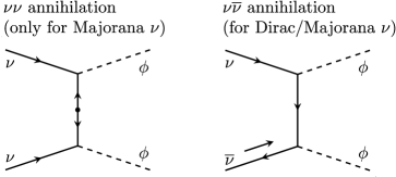
In the non-relativistic case the cross sections read (see Appendix H for details of the calculation):

	$\displaystyle\sigma^{\nu\bar{\nu}}\equiv\sigma(\nu+\overline{\nu}\rightarrow\phi+\phi)$	$\displaystyle\approx\frac{3vy^{4}}{16\pi m_{\nu}^{2}}\thinspace,$		(169)
	$\displaystyle\sigma^{\nu\nu}\equiv\sigma(\nu+\nu\rightarrow\phi+\phi)$	$\displaystyle\approx\frac{y^{4}}{4\pi m_{\nu}^{2}v}\thinspace,$		(170)

where $v$ is the relative velocity of colliding neutrinos:

v=\sqrt{v_{1}^{2}+v_{2}^{2}-2v_{1}v_{2}\cos\theta_{12}}\thinspace,

and $v_{i}=|\mathbf{p}_{i}|/m_{\nu}$ ( $i=1,2$ ) are the velocities of the colliding neutrinos and $\theta_{12}$ the angle between $\mathbf{p}_{1}$ and $\mathbf{p}_{2}$ .

The key difference is dependence on $v$ : $\sigma^{\nu\bar{\nu}}\propto v$ , while $\sigma^{\nu\nu}\propto v^{-1}$ . For the Majorana case (both $\nu+\overline{\nu}$ and $\nu+\nu$ channels are present) in the limit $v\ll 1$ , the left diagram dominates. Hence for Dirac or Majorana neutrinos, one only needs to consider $\nu+\overline{\nu}$ or $\nu+\nu$ annihilation, respectively.

The change of number density due to annihilation can be computed as

\frac{dn}{dt}=-\int f_{1}(\mathbf{p}_{1})f_{2}(\mathbf{p}_{2})\sigma(v)v\frac{d^{3}\mathbf{p}_{1}}{(2\pi)^{3}}\frac{d^{3}\mathbf{p}_{2}}{(2\pi)^{3}}\thinspace,

(171)

where $f_{1}$ and $f_{2}$ are the distribution functions of the initial neutrinos. Introducing integration over velocities the rate (171) becomes

\frac{dn}{dt}=-\int f_{1}f_{2}\sigma(v)v\frac{m_{\nu}^{3}4\pi v_{1}^{2}dv_{1}}{(2\pi)^{3}}\frac{m_{\nu}^{3}2\pi v_{2}^{2}dv_{2}d\cos\theta_{12}}{(2\pi)^{3}}\thinspace,

The result reads

\displaystyle\frac{dn^{\nu\bar{\nu}}}{dt}

\displaystyle\approx-\frac{p_{F}^{8}y^{4}}{160\pi^{5}m_{\nu}^{4}},\leavevmode\nobreak\ \leavevmode\nobreak\ \leavevmode\nobreak\ \leavevmode\nobreak\ \leavevmode\nobreak\ \frac{dn^{\nu\nu}}{dt}\approx-\frac{p_{F}^{6}y^{4}}{144\pi^{5}m_{\nu}^{2}}.\

(172)

Using Eq. (31), we express the number density $n$ in terms of $p_{F}$ , thus obtaining the differential equation for $p_{F}$ :

	$\displaystyle\frac{dp_{F}^{\nu\bar{\nu}}}{dt}$	$\displaystyle=-\frac{p_{F}^{6}y^{4}}{80\pi^{3}m_{\nu}^{4}}\,,$		(173)
	$\displaystyle\frac{dp_{F}^{\nu\nu}}{dt}$	$\displaystyle=-\frac{p_{F}^{4}y^{4}}{72\pi^{3}m_{\nu}^{2}}\,,$		(174)

The solution is

	$\displaystyle p_{F}^{\nu\bar{\nu}}(t)$	$\displaystyle=p_{F}^{0}\left[1+\frac{p_{F0}^{5}y^{4}}{16\pi^{3}m_{\nu}^{4}}t\right]^{-1/5}\,,$		(175)
	$\displaystyle p_{F}^{\nu\nu}(t)$	$\displaystyle=p_{F}^{0}\left[1+\frac{p_{F0}^{3}y^{4}}{24\pi^{3}m_{\nu}^{2}}t\right]^{-1/3}\,,$		(176)

where $p_{F}^{0}$ is the Fermi momentum in the beginning of the cooling phase. The annihilation lifetime $\tau_{{\rm anni}}$ can be defined as the time during which the Fermi momentum reduces by a factor of 2: $p_{F}(\tau_{{\rm anni}})=p_{F}^{0}/2$ , which corresponds to the density being reduced by a factor of 8. Then from (175) and (176) we obtain

	$\displaystyle\tau^{\nu\bar{\nu}}$	$\displaystyle=\frac{496\pi^{3}m_{\nu}^{4}}{y^{4}p_{F0}^{5}}=1.0\times 10^{23}\text{seconds}\times\left(\frac{0.1\ {\rm eV}}{m_{\nu}}\right)\left(\frac{0.1m_{\nu}}{p_{F0}}\right)^{5}\left(\frac{10^{-7}}{y}\right)^{4},$		(177)
	$\displaystyle\tau^{\nu\nu}$	$\displaystyle=\frac{168\pi^{3}m_{\nu}^{2}}{y^{4}p_{F0}^{3}}=3.4\times 10^{20}\text{seconds}\times\left(\frac{0.1\ {\rm eV}}{m_{\nu}}\right)\left(\frac{0.1m_{\nu}}{p_{F0}}\right)^{3}\left(\frac{10^{-7}}{y}\right)^{4}.$		(178)

Therefore for typical values of parameters presented in Eqs. (177) and (178), one finds that that $\tau_{{\rm anni}}\gg\tau_{\text{universe}}=4.35\times 10^{17}{\rm seconds}$ .

Acknowledgements.

The authors would like to thank Julian Heeck and Arvind Rajaraman for useful discussions on this topic in 2019, Jerome Vandecasteele and Peter Tinyakov for discussions on similar fermionic systems in neutron stars, and Laura Lopez Honorez for suggesting references. X.J.X is supported in part by the National Natural Science Foundation of China under grant No. 12141501.

References

Samanta (2011) A. Samanta, JCAP 1109, 010 (2011), arXiv:1001.5344 [hep-ph] .
Heeck and Rodejohann (2011) J. Heeck and W. Rodejohann, J. Phys. G38, 085005 (2011), arXiv:1007.2655 [hep-ph] .
Wise and Zhang (2018) M. B. Wise and Y. Zhang, JHEP 06, 053 (2018), arXiv:1803.00591 [hep-ph] .
Bustamante and Agarwalla (2019) M. Bustamante and S. K. Agarwalla, Phys. Rev. Lett. 122, 061103 (2019), arXiv:1808.02042 [astro-ph.HE] .
Smirnov and Xu (2019) A. Y. Smirnov and X.-J. Xu, JHEP 12, 046 (2019), arXiv:1909.07505 [hep-ph] .
Babu et al. (2020) K. S. Babu, G. Chauhan, and P. S. Bhupal Dev, Phys. Rev. D 101, 095029 (2020), arXiv:1912.13488 [hep-ph] .
Boehm et al. (2012) C. Boehm, M. J. Dolan, and C. McCabe, JCAP 12, 027 (2012), arXiv:1207.0497 [astro-ph.CO] .
Heeck (2014) J. Heeck, Phys. Lett. B 739, 256 (2014), arXiv:1408.6845 [hep-ph] .
Huang et al. (2018) G.-y. Huang, T. Ohlsson, and S. Zhou, Phys. Rev. D 97, 075009 (2018), arXiv:1712.04792 [hep-ph] .
Luo et al. (2021) X. Luo, W. Rodejohann, and X.-J. Xu, JCAP 03, 082 (2021), arXiv:2011.13059 [hep-ph] .
Esteban and Salvado (2021) I. Esteban and J. Salvado, (2021), arXiv:2101.05804 [hep-ph] .
Green et al. (2021) D. Green, D. E. Kaplan, and S. Rajendran, JHEP 11, 162 (2021), arXiv:2108.06928 [hep-ph] .
Markov (1964) M. A. Markov, Phys. Lett. 10, 122 (1964).
Viollier et al. (1993) R. D. Viollier, D. Trautmann, and G. B. Tupper, Phys. Lett. B 306, 79 (1993).
Bilic et al. (1999) N. Bilic, F. Munyaneza, and R. D. Viollier, Phys. Rev. D 59, 024003 (1999), arXiv:astro-ph/9801262 .
Bilic et al. (2001) N. Bilic, R. J. Lindebaum, G. B. Tupper, and R. D. Viollier, Phys. Lett. B 515, 105 (2001), arXiv:astro-ph/0106209 .
Stephenson et al. (1998) G. J. Stephenson, Jr., J. T. Goldman, and B. H. J. McKellar, Int. J. Mod. Phys. A 13, 2765 (1998), arXiv:hep-ph/9603392 .
Stephenson and Goldman (1993) G. J. Stephenson, Jr. and J. T. Goldman, (1993), arXiv:hep-ph/9309308 .
Wise and Zhang (2014) M. B. Wise and Y. Zhang, Phys. Rev. D 90, 055030 (2014), [Erratum: Phys.Rev.D 91, 039907 (2015)], arXiv:1407.4121 [hep-ph] .
Wise and Zhang (2015) M. B. Wise and Y. Zhang, JHEP 02, 023 (2015), [Erratum: JHEP 10, 165 (2015)], arXiv:1411.1772 [hep-ph] .
Gresham et al. (2017) M. I. Gresham, H. K. Lou, and K. M. Zurek, Phys. Rev. D 96, 096012 (2017), arXiv:1707.02313 [hep-ph] .
Gresham et al. (2018) M. I. Gresham, H. K. Lou, and K. M. Zurek, Phys. Rev. D 98, 096001 (2018), arXiv:1805.04512 [hep-ph] .
Chikashige et al. (1981) Y. Chikashige, R. N. Mohapatra, and R. D. Peccei, Phys. Lett. 98B, 265 (1981).
Griffiths (2016) D. Griffiths, Introduction to Quantum Mechanics (Cambridge University Press, 2016).
Chandrasekhar and Chandrasekhar (1957) S. Chandrasekhar and S. Chandrasekhar, An Introduction to the Study of Stellar Structure, Astrophysical monographs (Dover Publications, 1957).
Mota and van de Bruck (2004) D. F. Mota and C. van de Bruck, Astron. Astrophys. 421, 71 (2004), arXiv:astro-ph/0401504 .
Baracchini et al. (2018) E. Baracchini et al. (PTOLEMY), (2018), arXiv:1808.01892 [physics.ins-det] .
Betti et al. (2019) M. G. Betti et al. (PTOLEMY), JCAP 07, 047 (2019), arXiv:1902.05508 [astro-ph.CO] .
Berryman et al. (2018) J. M. Berryman, A. De Gouvea, K. J. Kelly, and Y. Zhang, Phys. Rev. D97, 075030 (2018), arXiv:1802.00009 [hep-ph] .
Agostini et al. (2015) M. Agostini et al., Eur. Phys. J. C75, 416 (2015), arXiv:1501.02345 [nucl-ex] .
Brdar et al. (2020) V. Brdar, M. Lindner, S. Vogl, and X.-J. Xu, Phys. Rev. D 101, 115001 (2020), arXiv:2003.05339 [hep-ph] .
Forastieri et al. (2015) F. Forastieri, M. Lattanzi, and P. Natoli, JCAP 1507, 014 (2015), arXiv:1504.04999 [astro-ph.CO] .
Kachelriess et al. (2000) M. Kachelriess, R. Tomas, and J. W. F. Valle, Phys. Rev. D62, 023004 (2000), arXiv:hep-ph/0001039 [hep-ph] .
Farzan (2003) Y. Farzan, Phys. Rev. D67, 073015 (2003), arXiv:hep-ph/0211375 [hep-ph] .
Barger et al. (1982) V. D. Barger, W.-Y. Keung, and S. Pakvasa, Phys. Rev. D25, 907 (1982).
Lessa and Peres (2007) A. P. Lessa and O. L. G. Peres, Phys. Rev. D75, 094001 (2007), arXiv:hep-ph/0701068 [hep-ph] .
Pasquini and Peres (2016) P. S. Pasquini and O. L. G. Peres, Phys. Rev. D93, 053007 (2016), [Erratum: Phys. Rev.D93,no.7,079902(2016)], arXiv:1511.01811 [hep-ph] .
Burgess and Cline (1993) C. P. Burgess and J. M. Cline, Phys. Lett. B298, 141 (1993), arXiv:hep-ph/9209299 [hep-ph] .
Burgess and Cline (1994) C. P. Burgess and J. M. Cline, Phys. Rev. D49, 5925 (1994), arXiv:hep-ph/9307316 [hep-ph] .
Blum et al. (2018) K. Blum, Y. Nir, and M. Shavit, Phys. Lett. B785, 354 (2018), arXiv:1802.08019 [hep-ph] .
Cepedello et al. (2019) R. Cepedello, F. F. Deppisch, L. Gonzalez, C. Hati, and M. Hirsch, Phys. Rev. Lett. 122, 181801 (2019), arXiv:1811.00031 [hep-ph] .
Brune and Paes (2019) T. Brune and H. Paes, Phys. Rev. D99, 096005 (2019), arXiv:1808.08158 [hep-ph] .
Deppisch et al. (2020) F. F. Deppisch, L. Graf, W. Rodejohann, and X.-J. Xu, Phys. Rev. D 102, 051701 (2020), arXiv:2004.11919 [hep-ph] .
Bilmis et al. (2015) S. Bilmis, I. Turan, T. M. Aliev, M. Deniz, L. Singh, and H. T. Wong, Phys. Rev. D 92, 033009 (2015), arXiv:1502.07763 [hep-ph] .
Lindner et al. (2018) M. Lindner, F. S. Queiroz, W. Rodejohann, and X.-J. Xu, JHEP 05, 098 (2018), arXiv:1803.00060 [hep-ph] .
Adelberger et al. (2007) E. G. Adelberger, B. R. Heckel, S. A. Hoedl, C. D. Hoyle, D. J. Kapner, and A. Upadhye, Phys. Rev. Lett. 98, 131104 (2007), arXiv:hep-ph/0611223 .
Adelberger et al. (2009) E. G. Adelberger, J. H. Gundlach, B. R. Heckel, S. Hoedl, and S. Schlamminger, Prog. Part. Nucl. Phys. 62, 102 (2009).
Wagner et al. (2012) T. A. Wagner, S. Schlamminger, J. H. Gundlach, and E. G. Adelberger, Class. Quant. Grav. 29, 184002 (2012), arXiv:1207.2442 [gr-qc] .
Xu (2020) X.-J. Xu, JHEP 09, 105 (2020), arXiv:2007.01893 [hep-ph] .
Chauhan and Xu (2021) G. Chauhan and X.-J. Xu, JHEP 04, 003 (2021), arXiv:2012.09980 [hep-ph] .
Dent et al. (2012) J. B. Dent, F. Ferrer, and L. M. Krauss, (2012), arXiv:1201.2683 [astro-ph.CO] .
Kazanas et al. (2014) D. Kazanas, R. N. Mohapatra, S. Nussinov, V. L. Teplitz, and Y. Zhang, Nucl. Phys. B 890, 17 (2014), arXiv:1410.0221 [hep-ph] .
Heurtier and Zhang (2017) L. Heurtier and Y. Zhang, JCAP 02, 042 (2017), arXiv:1609.05882 [hep-ph] .
Dev et al. (2020) P. S. B. Dev, R. N. Mohapatra, and Y. Zhang, JCAP 08, 003 (2020), [Erratum: JCAP 11, E01 (2020)], arXiv:2005.00490 [hep-ph] .

$\displaystyle a_{\mathbf{p}}^{s}\|w\rangle$	$\displaystyle=a_{\mathbf{p}}^{s}\int\frac{d^{3}p^{\prime}}{(2\pi)^{3}}w(\mathbf{p}^{\prime})a_{\mathbf{p}^{\prime}}^{s\dagger}\|0\rangle$
	$\displaystyle=\int d^{3}\mathbf{p}^{\prime}\thinspace w(\mathbf{p}^{\prime})\delta^{3}(\mathbf{p}-\mathbf{p}^{\prime})\|0\rangle$
	$\displaystyle=w(\mathbf{p})\|0\rangle.$	(104)

$\displaystyle\langle w\|\psi^{\dagger}(x)\psi(x)\|w\rangle$	$\displaystyle=\int\frac{d^{3}\mathbf{k}}{(2\pi)^{3}}\frac{d^{3}\mathbf{p}}{(2\pi)^{3}}\frac{1}{\sqrt{2E_{\mathbf{k}}}\sqrt{2E_{\mathbf{p}}}}\langle w\|a_{\mathbf{k}}^{s\dagger}u^{s\dagger}(k)e^{ik\cdot x}a_{\mathbf{p}}^{s}u^{s}(p)e^{-ip\cdot x}\|w\rangle$
	$\displaystyle=\int\frac{d^{3}\mathbf{k}}{(2\pi)^{3}}\frac{d^{3}\mathbf{p}}{(2\pi)^{3}}\frac{u^{s\dagger}(k)u^{s}(p)}{\sqrt{2E_{\mathbf{k}}}\sqrt{2E_{\mathbf{p}}}}e^{i(k-p)\cdot x}\langle 0\|w(\mathbf{k})^{*}w(\mathbf{p})\|0\rangle$
	$\displaystyle=\Psi^{\dagger}(x)\Psi(x),$	(105)

Neutrino bound states and bound systems

Abstract

I Introduction

II Yukawa potential for neutrinos

III Two-neutrino bound states

III.1 Quantitative study

III.2 Coulomb limit

III.3 Approximate solutions for non-zero mass of scalar from the variation principle

IV NN-neutrino bound systems

IV.1 Qualitative estimation

IV.2 Quantitative study

IV.3 Non-degenerate ν\nu-clusters

V Relativistic regime

V.1 Equations for degenerate neutrino cluster

V.2 Solution for massless mediator

V.3 Neutrino clusters for nonzero mϕm_{\phi}

V.4 Neutrino bound systems for given yy and mϕm_{\phi}

VI Formation of neutrino clusters

VI.1 Maximal density and fragmentation of the ν\nu background

VI.2 Evolution of the effective neutrino mass

VI.3 Energy of the ν\nu-ϕ\phi system and the dip

VI.4 Fragmentation

VI.5 Virialization

VI.6 Neutrino structure of the Universe

VII Conclusions

Appendix A Calculation of ⟨ψ¯​ψ⟩\langle\overline{\psi}\psi\rangle and ⟨ψ†​ψ⟩\langle\psi^{\dagger}\psi\rangle

Appendix B Potential issues on the binding energy and the field energy

Appendix C Numerical method to solve the two-particle Schrödinger equation

Appendix D Known constraints on the yukawa coupling

Appendix E Equivalence between chemical equilibrium and force balance

Appendix F Derivation of the Lane-Emden equation from equations of motion

Appendix G Numerical details of solving Eqs. (60) and (61)

Appendix H Annihilation cross sections

Appendix I Energy loss due to ϕ\phi bremsstrahlung

Appendix J Annihilation

Acknowledgements.

References

IV $N$ -neutrino bound systems

IV.3 Non-degenerate $\nu$ -clusters

V.3 Neutrino clusters for nonzero $m_{\phi}$

V.4 Neutrino bound systems for given $y$ and $m_{\phi}$

VI.1 Maximal density and fragmentation of the $\nu$ background

VI.3 Energy of the $\nu$ - $\phi$ system and the dip

Appendix A Calculation of $\langle\overline{\psi}\psi\rangle$ and $\langle\psi^{\dagger}\psi\rangle$

Appendix I Energy loss due to $\phi$ bremsstrahlung