New analysis of Mixed finite element methods for incompressible Magnetohydrodynamics

Yuchen Huang Advanced Institute of Natural Sciences, Beijing Normal University, Zhuhai 519087, P.R. China. , Weifeng Qiu Department of Mathematics, City University of Hong Kong, 83 Tat Chee Avenue, Kowloon, Hong Kong, China (weifeqiu@cityu.edu.hk). and Weiwei Sun Research Center for Mathematics, Advanced Institute of Natural Science, Beijing Normal University, Zhuhai, P.R. China Guangdong Provincial Key Laboratory of Interdisciplinary Research and Application for Data Science (IRADS), BNU-HKBU United International College, Zhuhai, 519087, P.R.China (W.Sun, maweiw@uic.edu.cn).

Abstract.

This paper focuses on new error analysis of a class of mixed FEMs for stationary incompressible magnetohydrodynamics with the standard inf-sup stable velocity-pressure space in cooperation with Navier-Stokes equations and the Nédélec’s edge element for the magnetic field. The methods have been widely used in various numerical simulations in the last several decades, while the existing analysis is not optimal due to the strong coupling of system and the pollution of the lower-order Nédélec’s edge approximation in analysis. In terms of a newly modified Maxwell projection we establish new and optimal error estimates. In particular, we prove that the method based on the commonly-used Taylor-Hood/lowest-order Nédélec’s edge element is efficient and the method provides the second-order accuracy for numerical velocity. Two numerical examples for the problem in both convex and nonconvex polygonal domains are presented, which confirm our theoretical analysis.

Key words and phrases:

Mixed method, Magnetohydrodynamics

2000 Mathematics Subject Classification:

65N30, 65L12

The work of W. Qiu was supported by a grant from the Research Grants Council of the Hong Kong Special Administrative Region, China (Project No. CityU 11302718).

The work of Y. Huang and W. Sun was partially supported by National Natural Science Foundation of China (12231003 and 12071040), Guangdong Provincial Key Laboratory IRADS (2022B1212010006, UIC-R0400001-22) and Guangdong Higher Education Upgrading Plan (UIC-R0400024-21).

1. Introduction

Magnetohydrodynamics (MHD) is the study of the interaction between electrically conducting fluids and electromagnetic fields [7, 15, 33], such as liquid metals, and salt water or electrolytes. Some more comprehensive discussion on the applications can be found in [15, 25, 32] and references therein. In this paper, we consider the steady state incompressible MHD model on $\Omega\subset\mathbb{R}^{d}$ , $d=2,3$ , defined by


$\displaystyle-R_{e}^{-1}\Delta{\boldsymbol{u}}+({\boldsymbol{u}}\cdot\nabla){\boldsymbol{u}}+\nabla p-S(\nabla\times{\boldsymbol{b}})\times{\boldsymbol{b}}$	$\displaystyle={\boldsymbol{f}}\quad\text{ in }\Omega,$	(1.1a)
$\displaystyle SR_{m}^{-1}\nabla\times(\nabla\times{\boldsymbol{b}})-S\nabla\times({\boldsymbol{u}}\times{\boldsymbol{b}})-\nabla r$	$\displaystyle={\boldsymbol{g}}\quad\text{ in }\Omega,$	(1.1b)
$\displaystyle\nabla\cdot{\boldsymbol{u}}$	$\displaystyle=0\quad\text{ in }\Omega,$	(1.1c)
$\displaystyle\nabla\cdot{\boldsymbol{b}}$	$\displaystyle=0\quad\text{ in }\Omega,$	(1.1d)
$\displaystyle{\boldsymbol{u}}$	$\displaystyle=\boldsymbol{0}\quad\text{ on }\partial\Omega,$	(1.1e)
$\displaystyle{\boldsymbol{n}}\times{\boldsymbol{b}}$	$\displaystyle=\boldsymbol{0}\quad\text{ on }\partial\Omega,$	(1.1f)
$\displaystyle r$	$\displaystyle=0\quad\text{ on }\partial\Omega,$	(1.1g)
$\displaystyle\int_{\Omega}p\,d{\boldsymbol{x}}$	$\displaystyle=0,$	(1.1h)

where $\Omega$ a simply-connected Lipschitz polygonal or polyhedral domain and ${\boldsymbol{n}}$ is the unit outward normal vector on $\partial\Omega$ . The solution of the above system consists of the velocity ${\boldsymbol{u}}$ , the pressure $p$ , the magnetic field ${\boldsymbol{b}}$ and the Lagrange multiplier $r$ associated with the divergence constraint on the magnetic field ${\boldsymbol{b}}$ . The above equations are characterized by three dimensionless parameters: the hydrodynamic Reynolds number $R_{e}$ , the magnetic Reynolds number $R_{m}$ and the coupling number $S$ . [2, 7, 15] provide detailed discussion of these parameters and their typical values.

Numerical methods and analysis for the MHD model have been investigated extensively in the last several decades, see [3, 14, 15, 16, 17, 19, 21, 23, 24, 31, 40, 43] and references therein. The model is described by a coupled system of electrical fluid flows and electromagnetic fields, governed by Navier-Stokes and Maxwell type equations, respectively. Therefore, numerical methods for the MHD system are based on a combination of the approximation to Navier-Stokes equations and the approximation to Maxwell equations. Earlier works was mainly focused on the classical Lagrange type finite element approximation to the magnetic field ${\boldsymbol{b}}$ . Analysis has been done by many authors [10, 14, 17, 19, 31]. [17] firstly provides the existence, uniqueness, and optimal convergent finite element approximation to the MHD system with nonhomogeneous boundary conditions. Instead of assuming the source terms $\boldsymbol{f}$ and $\boldsymbol{g}$ are small enough, the analysis in [17] only requires that $\|{\boldsymbol{u}}\|_{H^{\frac{1}{2}}(\partial\Omega)}$ is small enough (see [17, ( $4.19$ )]). A more popular approximation to Maxwell equations is the $H(\text{curl})$ -conforming Nédélec’s edge element methods, which have been widely used in many engineering areas. It is well-known that Lagrange type approximation may produce wrong numerical solutions for Maxwell equations in a nonconvex polyhedral domain, (see [1, 5]). For the MHD system, a class of mixed finite element methods was first presented by Schötzau [40], where the hydrodynamic system is discretized by standard inf-sup stable velocity-pressure space pairs and the magnetic system by a mixed approach using Nédélec’s elements of the first kind. Error estimates of methods were presented and the problem was considered in general domains. Subsequently, numerous efforts have been made with the Nédélec FE approximation [27, 30, 35, 37, 41, 42, 43] and the analysis has been extended to many different models and approximations [8, 9, 12, 22, 28, 36]. For a convex polyhedral domain, the main result given in [40] is the following error estimate

\displaystyle\|{\boldsymbol{u}}-{\boldsymbol{u}}_{h}\|_{H^{1}(\Omega)}+\|{\boldsymbol{b}}-{\boldsymbol{b}}_{h}\|_{H(\text{curl},\Omega)}\leq C(h^{l}+h^{k})

(1.2)

for the method with the approximation accuracy $O(h^{l})$ for hydrodynamic variables and the approximation accuracy $O(h^{k})$ for the magnetic field ${\boldsymbol{b}}$ . By (1.2), one has to take the combination with $k=l$ to achieve an optimal convergence rate. However, the method with $k<l$ is more popular since high-order Nédélec’s edge elements are more complicated in implementation and extremely time-consuming in computation. In particular, the method based on the combination of the Taylor-Hood element and the lowest-order Nédélec’s edge element has been frequently used in applications and numerical simulations have been done extensively [11, 39, 41, 42]. In this case, $k=1$ and $l=2$ , the error estimate (1.2) reduces to

\displaystyle\|{\boldsymbol{u}}-{\boldsymbol{u}}_{h}\|_{H^{1}(\Omega)}+\|{\boldsymbol{b}}-{\boldsymbol{b}}_{h}\|_{H(\text{curl},\Omega)}\leq C(h^{2}+h)\,.

(1.3)

One can see from (1.3) that the accuracy of numerical velocity is only of the first-order, which is not optimal in the traditional sense and also, not a good indication for the commonly-used method. It was assumed that the accuracy of the velocity is polluted by the lower-order Nédélec’s edge finite element approximation. This is a common question in many applications when FEMs with combined approximations of different orders is used for a strongly coupled system. The main purpose of this paper is to establish the optimal error estimate

\displaystyle\|{\boldsymbol{u}}-{\boldsymbol{u}}_{h}\|_{H^{1}(\Omega)}\leq C(h^{l}+h^{k+1})

(1.4)

for the standard combination, which shows that the numerical velocity is of one-order higher accuracy than given in previous analysis for the case $k<l$ and which implies the second-order accuracy

\displaystyle\|{\boldsymbol{u}}-{\boldsymbol{u}}_{h}\|_{H^{1}(\Omega)}\leq Ch^{2}

(1.5)

for the combination of Taylor-Hood element and the lowest-order Nédélec’s edge element of the first type. Our analysis is based on a new modified Maxwell projection. In terms of the projection and the error estimate in a negative norm, a more precise analysis is presented in this paper. The analysis shows clearly that the mixed method with the Taylor-Hood/lowest-order Nédélec’s edge element approximations is efficient and the method provides second-order accuracy for numerical velocity. The lower-order approximation to the magnetic field ${\boldsymbol{b}}$ does not influence the accuracy of numerical solution of Navier-Stokes equations.

The rest of the paper is organized as follows. In Section 2 we first provide the variational formulation and the mixed method for the MHD model and some existing results and then, we present our main theorem for an optimal error estimate of the method. To prove it, we introduce a modified Maxwell projection and establish its approximation properties in Section 3. In terms of this projection, we present our theoretical analysis. In section 4, we provide numerical experiments to confirm our theoretical analysis and show the efficiency of the method.

2. Mixed FEMs and main results

2.1. Mixed FEMs

To introduce the mixed method, we adopt the notations and norms used in [40, 43]. We denote some standard vector and scalar function spaces by

	$\displaystyle H(\text{curl},\Omega)=$	$\displaystyle\{{\boldsymbol{c}}\in[L^{2}(\Omega)]^{d}:\nabla\times{\boldsymbol{c}}\in[L^{2}(\Omega)]^{d}\},$
	$\displaystyle H_{0}(\text{curl},\Omega)=$	$\displaystyle\{{\boldsymbol{c}}\in H(\text{curl},\Omega):{\boldsymbol{n}}\times{\boldsymbol{c}}\|_{\partial\Omega}=\boldsymbol{0}\},$
	$\displaystyle{\boldsymbol{X}}=$	$\displaystyle\{{\boldsymbol{c}}\in H_{0}(\text{curl},\Omega):\nabla\cdot{\boldsymbol{c}}=0\},$
	$\displaystyle H(\text{div},\Omega)=$	$\displaystyle\{{\boldsymbol{c}}\in[L^{2}(\Omega)]^{d}:\nabla\cdot{\boldsymbol{c}}\in[L^{2}(\Omega)]^{d}\},$
	$\displaystyle L_{0}^{2}(\Omega)=$	$\displaystyle\{q\in L^{2}(\Omega):\int_{\Omega}qd{\boldsymbol{x}}=0\},$
	$\displaystyle H^{-1}(\Omega)=$	$\displaystyle\left(H_{0}^{1}(\Omega)\right)^{*}.$

For any $({\boldsymbol{v}},{\boldsymbol{c}})\in[H_{0}^{1}(\Omega)]^{d}\times H(\text{curl},\Omega)$ , we define

\displaystyle\|({\boldsymbol{v}},{\boldsymbol{c}})\|^{2}:=\|\nabla{\boldsymbol{v}}\|_{L^{2}(\Omega)}^{2}+S\|{\boldsymbol{c}}\|_{H(\text{curl},\Omega)}^{2}.

(2.1)

Moreover, we denote some bilinear or trilinear forms by

	$\displaystyle a_{s}({\boldsymbol{u}},{\boldsymbol{v}})=R_{e}^{-1}(\nabla{\boldsymbol{u}},\nabla{\boldsymbol{v}})_{\Omega},$
	$\displaystyle a_{m}({\boldsymbol{b}},{\boldsymbol{c}})=SR_{m}^{-1}(\nabla\times{\boldsymbol{b}},\nabla\times{\boldsymbol{c}})_{\Omega},$
	$\displaystyle c_{0}({\boldsymbol{w}};{\boldsymbol{u}},{\boldsymbol{v}})=\frac{1}{2}({\boldsymbol{w}}\cdot\nabla{\boldsymbol{u}},{\boldsymbol{v}})_{\Omega}-\frac{1}{2}({\boldsymbol{w}}\cdot\nabla{\boldsymbol{v}},{\boldsymbol{u}})_{\Omega},$
	$\displaystyle c_{1}({\boldsymbol{d}};{\boldsymbol{v}},{\boldsymbol{c}})=S((\nabla\times{\boldsymbol{c}})\times{\boldsymbol{d}},{\boldsymbol{v}})_{\Omega}=-S({\boldsymbol{v}}\times{\boldsymbol{d}},\nabla\times{\boldsymbol{c}})_{\Omega},$

for any ${\boldsymbol{u}},{\boldsymbol{v}}\in[H_{0}^{1}(\Omega)]^{d}$ and any ${\boldsymbol{b}},{\boldsymbol{c}},{\boldsymbol{d}}\in H_{0}(\text{curl},\Omega)$ with ${\boldsymbol{d}}\in[L^{3}(\Omega)]^{d}$ .

The exact solution $({\boldsymbol{u}},{\boldsymbol{b}},p,r)$ of the MHD system (1.1) satisfies the variational formulation


$\displaystyle a_{s}({\boldsymbol{u}},{\boldsymbol{v}})+c_{0}({\boldsymbol{u}};{\boldsymbol{u}},{\boldsymbol{v}})-c_{1}({\boldsymbol{b}};{\boldsymbol{v}},{\boldsymbol{b}})-(p,\nabla\cdot{\boldsymbol{v}})_{\Omega}=$	$\displaystyle({\boldsymbol{f}},{\boldsymbol{v}})_{\Omega},$	(2.2a)
$\displaystyle a_{m}({\boldsymbol{b}},{\boldsymbol{c}})+c_{1}({\boldsymbol{b}};{\boldsymbol{u}},{\boldsymbol{c}})-(\nabla r,{\boldsymbol{c}})_{\Omega}=$	$\displaystyle({\boldsymbol{g}},{\boldsymbol{c}})_{\Omega},$	(2.2b)
$\displaystyle(\nabla\cdot{\boldsymbol{u}},q)_{\Omega}=$	$\displaystyle 0,$	(2.2c)
$\displaystyle({\boldsymbol{b}},\nabla s)_{\Omega}=$	$\displaystyle 0,$	(2.2d)

for any $({\boldsymbol{v}},{\boldsymbol{c}},q,s)\in[H_{0}^{1}(\Omega)]^{d}\times H_{0}(\text{curl},\Omega)\times L_{0}^{2}(\Omega)\times H_{0}^{1}(\Omega)$ .

Let $\mathcal{T}_{h}$ denote a quasi-uniform conforming triangulation of $\Omega$ . On this triangulation, we define several finite element spaces by

	$\displaystyle{\boldsymbol{V}}_{h}^{l}$	$\displaystyle:=[H_{0}^{1}(\Omega)\cap P_{l}({\mathcal{T}}_{h})]^{d},$
	$\displaystyle\quad Q_{h}^{l}$	$\displaystyle:=P_{l-1}({\mathcal{T}}_{h})\cap H^{1}(\Omega)\cap L_{0}^{2}(\Omega),$
	$\displaystyle\quad{\boldsymbol{C}}_{h}^{k}$	$\displaystyle:=\{{\boldsymbol{c}}_{h}\in H_{0}(\text{curl},\Omega):{\boldsymbol{c}}_{h}\|_{K}\in[P_{k-1}(K)]^{d}\oplus D_{h}^{k}(K),\forall K\in{\mathcal{T}}_{h}\},$
	$\displaystyle\quad S_{h}^{k}$	$\displaystyle:=H_{0}^{1}(\Omega)\cap P_{k}({\mathcal{T}}_{h})$

for $l\geq 2$ and $k\geq 1$ , where $P_{l}({\mathcal{T}}_{h})=\{w\in L^{2}(\Omega):w|_{K}\in P_{l}(K),\forall K\in{\mathcal{T}}_{h}\}$ , $D_{h}^{k}(K)=\{{\boldsymbol{p}}\in[\tilde{P}_{k}(K)]^{d}:{\boldsymbol{p}}({\boldsymbol{x}})\cdot{\boldsymbol{x}}=0,\forall{\boldsymbol{x}}\in K\}$ and $\tilde{P}_{k}(K)$ is the collection of the $k$ -th order homogeneous polynomials in $P_{k}(K)$ . ${\boldsymbol{C}}_{h}^{k}$ is actually the $k$ -th order first type of Nédélec’s edge element space.

The mixed method in [40, 43] seeks an approximation $({\boldsymbol{u}}_{h},{\boldsymbol{b}}_{h},p_{h},r_{h})\in{\boldsymbol{V}}_{h}^{l}\times{\boldsymbol{C}}_{h}^{k}\times Q_{h}^{k}\times S_{h}^{l}$ to the exact solution $({\boldsymbol{u}},{\boldsymbol{b}},p,r)$ satisfying the following weak formulation:


$\displaystyle a_{s}({\boldsymbol{u}}_{h},{\boldsymbol{v}}_{h})+c_{0}({\boldsymbol{u}}_{h};{\boldsymbol{u}}_{h},{\boldsymbol{v}}_{h})-c_{1}({\boldsymbol{b}}_{h};{\boldsymbol{v}}_{h},{\boldsymbol{b}}_{h})-(p_{h},\nabla\cdot{\boldsymbol{v}}_{h})_{\Omega}$	$\displaystyle=({\boldsymbol{f}},{\boldsymbol{v}}_{h})_{\Omega},$	(2.3a)
$\displaystyle a_{m}({\boldsymbol{b}}_{h},{\boldsymbol{c}}_{h})+c_{1}({\boldsymbol{b}}_{h};{\boldsymbol{u}}_{h},{\boldsymbol{c}}_{h})-(\nabla r_{h},{\boldsymbol{c}}_{h})_{\Omega}$	$\displaystyle=({\boldsymbol{g}},{\boldsymbol{c}}_{h})_{\Omega},$	(2.3b)
$\displaystyle(\nabla\cdot{\boldsymbol{u}}_{h},q_{h})_{\Omega}$	$\displaystyle=0,$	(2.3c)
$\displaystyle({\boldsymbol{b}}_{h},\nabla s_{h})_{\Omega}$	$\displaystyle=0,$	(2.3d)

for all $({\boldsymbol{v}}_{h},{\boldsymbol{c}}_{h},q_{h},s_{h})\in{\boldsymbol{V}}_{h}^{l}\times{\boldsymbol{C}}_{h}^{k}\times Q_{h}^{l}\times S_{h}^{k}$ .

The paper is focused on optimal error estimates of the mixed method defined in (2.3). Iterative algorithms for solving the nonlinear algebraic system and their convergences were studied by several authors [10, 37, 41, 42, 43] and numerical simulations on various practical models can be found in literature [3, 11, 39]. Analysis presented in this paper can be extended to many other mixed methods.

2.2. Auxiliary results

The mixed method defined in (2.3a)-(2.3d) was analyzed by several authors. In this subsection, we provide some existing results which shall be used in our analysis.

Mimicking the space ${\boldsymbol{X}}$ defined at the beginning of Section 2.1, we introduce

\displaystyle{\boldsymbol{X}}_{h}:=\{{\boldsymbol{c}}_{h}\in{\boldsymbol{C}}_{h}^{k}:({\boldsymbol{c}}_{h},\nabla s_{h})_{\Omega}=0,\forall s_{h}\in S_{h}^{k}\}.

(2.4)

Lemma 2.1.

(see [43, ( $2.2$ , $2.3$ , $2.4$ )]) There exist positive constants $\lambda_{0},\lambda_{1}^{*},\lambda_{1}$ and $\lambda_{2}$ such that


		$\displaystyle\lambda_{0}\\|{\boldsymbol{c}}\\|_{H(\text{curl},\Omega)}\leq\\|\nabla\times{\boldsymbol{c}}\\|_{L^{2}(\Omega)},\quad\forall{\boldsymbol{c}}\in{\boldsymbol{X}},$		(2.5a)
		$\displaystyle\\|v\\|_{L^{3}(\Omega)}\leq\lambda_{1}^{*}\\|\nabla v\\|_{L^{2}(\Omega)},\quad\\|v\\|_{L^{6}(\Omega)}\leq\lambda_{1}\\|\nabla v\\|_{L^{2}(\Omega)},\quad\forall v\in H_{0}^{1}(\Omega),$		(2.5b)
		$\displaystyle\\|{\boldsymbol{c}}\\|_{L^{3}(\Omega)}\leq\lambda_{2}\\|\nabla\times{\boldsymbol{c}}\\|_{L^{2}(\Omega)},\quad\forall{\boldsymbol{c}}\in{\boldsymbol{X}}.$		(2.5c)

Lemma 2.2.

([43, Lemma $2.1$ ]) It holds that


$\displaystyle a_{s}({\boldsymbol{w}},{\boldsymbol{v}})+a_{m}({\boldsymbol{d}},{\boldsymbol{c}})\leq$	$\displaystyle\max\{R_{e}^{-1},R_{m}^{-1}\}\\|({\boldsymbol{w}},{\boldsymbol{d}})\\|\cdot\\|({\boldsymbol{v}},{\boldsymbol{c}})\\|,$	(2.6a)
	$\displaystyle\qquad\qquad\forall({\boldsymbol{w}},{\boldsymbol{d}}),({\boldsymbol{v}},{\boldsymbol{c}})\in[H_{0}^{1}(\Omega)]^{d}\times H_{0}(\text{curl},\Omega),$
$\displaystyle a_{s}({\boldsymbol{v}},{\boldsymbol{v}})+a_{m}({\boldsymbol{c}},{\boldsymbol{c}})\geq$	$\displaystyle\min(R_{e}^{-1},R_{m}^{-1}\lambda_{0})\\|({\boldsymbol{v}},{\boldsymbol{c}})\\|^{2},$	(2.6b)
	$\displaystyle\qquad\qquad\forall({\boldsymbol{v}},{\boldsymbol{c}})\in[H_{0}^{1}(\Omega)]^{d}\times{\boldsymbol{X}}$

and


$\displaystyle\sup_{{\boldsymbol{w}},\tilde{{\boldsymbol{v}}},{\boldsymbol{v}}\in[H_{0}^{1}(\Omega)]^{d}}\dfrac{c_{0}({\boldsymbol{w}};\tilde{{\boldsymbol{v}}},{\boldsymbol{v}})}{\\|\nabla{\boldsymbol{w}}\\|_{L^{2}(\Omega)}\\|\nabla\tilde{{\boldsymbol{v}}}\\|_{L^{2}(\Omega)}\\|\nabla{\boldsymbol{v}}\\|_{L^{2}(\Omega)}}=$	$\displaystyle\lambda_{1}\lambda_{1}^{*},$	(2.7a)
$\displaystyle\sup_{{\boldsymbol{d}}\in{\boldsymbol{X}},{\boldsymbol{v}}\in[H_{0}^{1}(\Omega)]^{d},{\boldsymbol{c}}\in H_{0}(\text{curl},\Omega)}\dfrac{c_{1}({\boldsymbol{d}};{\boldsymbol{v}},{\boldsymbol{c}})}{\\|{\boldsymbol{d}}\\|_{H(\text{curl},\Omega)}\\|\nabla{\boldsymbol{v}}\\|_{L^{2}(\Omega)}\\|{\boldsymbol{c}}\\|_{H(\text{curl},\Omega)}}=$	$\displaystyle S\lambda_{1}\lambda_{2},$	(2.7b)
$\displaystyle\sup_{{\boldsymbol{d}}\in{\boldsymbol{X}},\tilde{{\boldsymbol{c}}},{\boldsymbol{c}}\in H_{0}(\text{curl},\Omega),{\boldsymbol{w}},\tilde{{\boldsymbol{v}}},{\boldsymbol{v}}\in[H_{0}^{1}(\Omega)]^{d}}\dfrac{c_{0}({\boldsymbol{w}};\tilde{{\boldsymbol{v}}},{\boldsymbol{v}})-c_{1}({\boldsymbol{d}};{\boldsymbol{v}},\tilde{{\boldsymbol{c}}})+c_{1}({\boldsymbol{d}};\tilde{{\boldsymbol{v}}},{\boldsymbol{c}})}{\\|({\boldsymbol{w}},{\boldsymbol{d}})\\|\cdot\\|(\tilde{{\boldsymbol{v}}},\tilde{{\boldsymbol{c}}})\\|\cdot\\|({\boldsymbol{v}},{\boldsymbol{c}})\\|}=$	$\displaystyle\widehat{N}_{1}$	(2.7c)
$\displaystyle:=$	$\displaystyle\sqrt{2}\lambda_{1}\max\{\lambda_{1}^{*},\lambda_{2}\}.$

Here the constants $\lambda_{0},\lambda_{1}^{*},\lambda_{1}$ and $\lambda_{2}$ are introduced in Lemma 2.1.

For any $\lambda>0$ , we define

\displaystyle\eta(\lambda):=\dfrac{\left(\|{\boldsymbol{f}}\|_{L^{2}(\Omega)}+S^{-1}\|{\boldsymbol{g}}\|_{L^{2}(\Omega)}\right)}{\left(\min\{R_{e}^{-1},R_{m}^{-1}\lambda\}\right)^{2}}.

(2.8)

The well-posedness of the MHD system (1.1) is given in the following lemma and the proof can be found in [40, 43].

Lemma 2.3.

Suppose that

\displaystyle\widehat{N}_{1}\eta(\lambda_{0})<1,

(2.9)

where $\widehat{N}_{1}$ is introduced in (2.7c) and and $\eta(\lambda_{0})$ is defined as (2.8) with $\lambda=\lambda_{0}$ . Then the MHD system (1.1) admits a unique solution $({\boldsymbol{u}},{\boldsymbol{b}},p,r)\in[H_{0}^{1}(\Omega)]^{d}\times H_{0}(\text{curl},\Omega)\times L_{0}^{2}(\Omega)\times H_{0}^{1}(\Omega)$ satisfying

\displaystyle\|({\boldsymbol{u}},{\boldsymbol{b}})\|\leq\eta(\lambda_{0})\min\{R_{e}^{-1},R_{m}^{-1}\lambda_{0}\}\,.

(2.10)

Lemma 2.4.

([34, Lemma $7.20$ ], [38, Lemma $5.1$ ]) There exist positive constants $\lambda_{0}^{*},\lambda_{2}^{*}$ independent of $h$ such that

\displaystyle\lambda_{0}^{*}\|{\boldsymbol{c}}_{h}\|_{H(\text{curl},\Omega)}\leq\|\nabla\times{\boldsymbol{c}}_{h}\|_{L^{2}(\Omega)},\quad\|{\boldsymbol{c}}_{h}\|_{L^{3}(\Omega)}\leq\lambda_{2}^{*}\|\nabla\times{\boldsymbol{c}}_{h}\|_{L^{2}(\Omega)},\quad\forall{\boldsymbol{c}}_{h}\in{\boldsymbol{X}}_{h}

(2.11)

where the finite element space ${\boldsymbol{X}}_{h}$ is introduced in (2.4).

The well-posedness of the finite element system and error estimates of finite element solutions were presented in [40, 43]. With the above lemma, the well-posedness with a slightly weak condition is given in the following lemma. The proof follows those given in [40, 43] and is omitted here.

Lemma 2.5.

Supposed that

\displaystyle\widehat{N}_{2}\eta(\lambda_{0}^{*})<1,

(2.12)

where $\widehat{N}_{2}=\sqrt{2}\lambda_{1}\max\{\lambda_{1}^{*},\lambda_{2}^{*}\}$ and $\eta(\lambda_{0}^{*})$ is defined as (2.8) with $\lambda=\lambda_{0}^{*}$ . Then the mixed finite element system (2.3) admits a unique solution satisfying

\displaystyle\|({\boldsymbol{u}}_{h},{\boldsymbol{b}}_{h})\|\leq\eta(\lambda_{0}^{*})\min\{R_{e}^{-1},R_{m}^{-1}\lambda_{0}^{*}\}.

(2.13)

Here the constants $\lambda_{0}^{*},\lambda_{2}^{*}$ are introduced in Lemma 2.4, while $\lambda_{1},\lambda_{1}^{*}$ are defined in Lemma 2.1.

In addition,

\displaystyle\|{\boldsymbol{u}}-{\boldsymbol{u}}_{h}\|_{H^{1}(\Omega)}+\|{\boldsymbol{b}}-{\boldsymbol{b}}_{h}\|_{H(\text{curl},\Omega)}\leq C(h^{l}+h^{k})\,.

(2.14)

Remark 2.1.

We can see that the condition (2.12) and discrete inverse inequality implies the condition (2.9) and from (2.14) that

\displaystyle\|{\boldsymbol{u}}_{h}\|_{W^{1,p}(\Omega)}\leq C\qquad\mbox{ for }p\leq 6\,.

(2.15)

2.3. Main results

Under the assumptions of Lemma 2.3, the MHD system (1.1) is well-posed. We further assume that the solution satisfies the following regularity condition: there exists a positive constant $K$ , such that

	$\displaystyle\\|{\boldsymbol{b}}\\|_{W^{1,d^{+}}(\Omega)}+\\|\nabla\times{\boldsymbol{b}}\\|_{W^{1,d^{+}}(\Omega)}+\\|{\boldsymbol{u}}\\|_{H^{l+1}(\Omega)}$	$\displaystyle+\\|p\\|_{H^{l}(\Omega)}+\\|{\boldsymbol{b}}\\|_{H^{k}(\Omega)}$
		$\displaystyle+\\|\nabla\times{\boldsymbol{b}}\\|_{H^{k}(\Omega)}+\\|r\\|_{H^{k+1}(\Omega)}\leq K.$		(2.16)

Here $d^{+}$ denotes a constant strictly bigger than $d$ .

Our main result is the following Theorem 2.1.

Theorem 2.1.

We assume that the domain $\Omega$ is a convex polygon or polyhedra in $\mathbb{R}^{d}$ and the conditions (2.12, 2.16) hold. Then the mixed finite element system (2.3) admits a unique solution and there exists $h_{0}>0$ such that when $h\leq h_{0}$ ,

		$\displaystyle\\|{\boldsymbol{u}}-{\boldsymbol{u}}_{h}\\|_{H^{1}(\Omega)}+\\|\tilde{{\boldsymbol{b}}}_{h}-{\boldsymbol{b}}_{h}\\|_{H(\text{curl},\Omega)}\leq C_{1}\left(h^{l}+h^{k+1}\right),$		(2.17)
		$\displaystyle\\|{\boldsymbol{b}}-{\boldsymbol{b}}_{h}\\|_{H(\text{curl},\Omega)}\leq C_{1}\left(h^{l}+h^{k}\right),$

where $C_{1}$ is a positive constant depending upon the physical parameters $S,R_{m},R_{e}$ , the domain $\Omega$ and the constant $K$ introduced in (2.16). Here $\tilde{{\boldsymbol{b}}}_{h}\in{\boldsymbol{C}}_{h}^{k}$ is a projection of $({\boldsymbol{b}},r)$ defined below in (3.2).

Corollary 2.2.

Under the assumptions of Theorem 2.1, it holds that

\displaystyle\|{\boldsymbol{u}}-{\boldsymbol{u}}_{h}\|_{L^{2}(\Omega)}+\|{\boldsymbol{b}}-{\boldsymbol{b}}_{h}\|_{H^{-1}(\Omega)}\leq C_{2}\left(h^{l+1}+h^{k+1}\right),

(2.18)

where $C_{2}$ is a positive constant depending upon the physical parameters $S,R_{m},R_{e}$ , the domain $\Omega$ and the constant $K$ introduced in (2.16).

Remarks. For the Taylor-Hood/lowest-order Nédélec’s edge element of the first type, $l=2$ and $k=1$ . From the above theorem, one can see that the frequently-used mixed method provides the second-order accuracy for the numerical velocity, while only the first-order accuracy was presented in previous analyses. For the MINI/lowest-order Nédélec’s edge element of the first type, $l=k=1$ and the optimal error estimate of the second-order in $L^{2}$ -norm is shown in (2.18). For simplicity, hereafter we denote by $C_{K}$ a generic positive constant which depends upon $K$ .

3. Analysis

Before proving our main results, we present a modified Maxwell projection in the following subsection, which plays a key role in the proof of Theorem 2.1.

3.1. Projections

Let $(\tilde{{\boldsymbol{u}}}_{h},\tilde{p}_{h})\in{\boldsymbol{V}}_{h}^{l}\times Q_{h}^{l}$ be the standard Stokes projection of $({\boldsymbol{u}},p)$ defined by


$\displaystyle a_{s}({\boldsymbol{u}}-\tilde{{\boldsymbol{u}}}_{h},{\boldsymbol{v}}_{h})-(p-\tilde{p}_{h},\nabla\cdot{\boldsymbol{v}}_{h})_{\Omega}=$	$\displaystyle 0,\quad\forall{\boldsymbol{v}}_{h}\in{\boldsymbol{V}}_{h}^{l}$	(3.1a)
$\displaystyle(\nabla\cdot({\boldsymbol{u}}-\tilde{{\boldsymbol{u}}}_{h}),q_{h})_{\Omega}=$	$\displaystyle 0,\quad\forall q_{h}\in Q_{h}^{l}.$	(3.1b)

Let $(\tilde{{\boldsymbol{b}}}_{h},\tilde{r}_{h})\in{\boldsymbol{C}}_{h}^{k}\times S_{h}^{k}$ be the modified Maxwell projection of $({\boldsymbol{b}},r)$ defined by


$\displaystyle a_{m}({\boldsymbol{b}}-\tilde{{\boldsymbol{b}}}_{h},{\boldsymbol{c}}_{h})+c_{1}({\boldsymbol{b}}-\tilde{{\boldsymbol{b}}}_{h};{\boldsymbol{u}},{\boldsymbol{c}}_{h})-(\nabla(r-\tilde{r}_{h}),{\boldsymbol{c}}_{h})_{\Omega}=$	$\displaystyle 0,\quad\forall{\boldsymbol{c}}_{h}\in{\boldsymbol{C}}_{h}^{k},$	(3.2a)
$\displaystyle({\boldsymbol{b}}-\tilde{{\boldsymbol{b}}}_{h},\nabla s_{h})_{\Omega}=$	$\displaystyle 0,\quad\forall s_{h}\in S_{h}^{k}.$	(3.2b)

With the Stokes projection (3.1) and the modified Maxwell projection (3.2), we define an error splitting by


$\displaystyle{\boldsymbol{u}}-{\boldsymbol{u}}_{h}=$	$\displaystyle({\boldsymbol{u}}-\tilde{{\boldsymbol{u}}}_{h})+(\tilde{{\boldsymbol{u}}}_{h}-{\boldsymbol{u}}_{h}):=\xi_{{\boldsymbol{u}}}+e_{{\boldsymbol{u}}},$	(3.3a)
$\displaystyle{\boldsymbol{b}}-{\boldsymbol{b}}_{h}=$	$\displaystyle({\boldsymbol{b}}-\tilde{{\boldsymbol{b}}}_{h})+(\tilde{{\boldsymbol{b}}}_{h}-{\boldsymbol{b}}_{h}):=\xi_{{\boldsymbol{b}}}+e_{{\boldsymbol{b}}},$	(3.3b)
$\displaystyle p-p_{h}=$	$\displaystyle(p-\tilde{p}_{h})+(\tilde{p}_{h}-p_{h}):=\xi_{p}+e_{p},$	(3.3c)
$\displaystyle r-r_{h}=$	$\displaystyle(r-\tilde{r}_{h})+(\tilde{r}_{h}-r_{h}):=\xi_{r}+e_{r}.$	(3.3d)

Moreover, we denote by $(\widehat{{\boldsymbol{b}}}_{h},\widehat{r}_{h})\in{\boldsymbol{C}}_{h}^{k}\times S_{h}^{k}$ the standard Maxwell projection defined by


$\displaystyle a_{m}({\boldsymbol{b}}-\widehat{{\boldsymbol{b}}}_{h},{\boldsymbol{c}}_{h})-(\nabla(r-\widehat{r}_{h}),{\boldsymbol{c}}_{h})_{\Omega}=$	$\displaystyle 0,\quad\forall{\boldsymbol{c}}_{h}\in{\boldsymbol{C}}_{h}^{k},$	(3.4a)
$\displaystyle({\boldsymbol{b}}-\widehat{{\boldsymbol{b}}}_{h},\nabla s_{h})_{\Omega}=$	$\displaystyle 0,\quad\forall s_{h}\in S_{h}^{k}.$	(3.4b)

By classic finite element theory, we have the error estimates

\displaystyle\|\xi_{{\boldsymbol{u}}}\|_{L^{2}(\Omega)}+h(\|\nabla\xi_{{\boldsymbol{u}}}\|_{L^{2}(\Omega)}+\|\xi_{p}\|_{L^{2}(\Omega)})\leq Ch^{l+1}(\|{\boldsymbol{u}}\|_{H^{l+1}(\Omega)}+\|p\|_{H^{l}(\Omega)})

(3.5)

for the Stokes projection in (3.1) when $\Omega$ is convex and

	$\displaystyle\\|\nabla\times(\widehat{{\boldsymbol{b}}}_{h}-{\boldsymbol{b}})\\|_{L^{2}(\Omega)}$	$\displaystyle+\\|\widehat{{\boldsymbol{b}}}_{h}-{\boldsymbol{b}}\\|_{L^{2}(\Omega)}+\\|\nabla(\widehat{r}_{h}-r)\\|_{L^{2}(\Omega)}$
		$\displaystyle\leq Ch^{\min(k,s)}\left(\\|{\boldsymbol{b}}\\|_{H^{s}(\Omega)}+\\|\nabla\times{\boldsymbol{b}}\\|_{H^{s}(\Omega)}+\\|r\\|_{H^{s+1}(\Omega)}\right)$		(3.6)

for the Maxwell projection in (3.4). Here $s>0$ .

In order to provide the error estimates for the modified Maxwell projection, we consider $({\boldsymbol{z}},\phi)\in H_{0}(\text{curl},\Omega)\times H_{0}^{1}(\Omega)$ satisfying


$\displaystyle SR_{m}^{-1}\nabla\times(\nabla\times{\boldsymbol{z}})+S{\boldsymbol{u}}\times(\nabla\times{\boldsymbol{z}})-\nabla\phi=$	$\displaystyle{\boldsymbol{\theta}},$	(3.7a)
$\displaystyle\nabla\cdot{\boldsymbol{z}}=$	$\displaystyle 0,$	(3.7b)

where ${\boldsymbol{\theta}}\in[L^{2}(\Omega)]^{d}$ . The well-posedness of the above system is presented in the following theorem.

Theorem 3.1.

Suppose that (2.9) holds. Then the system (3.7) has a unique solution. If we further assume $\Omega$ is a convex polygon or polyhedra, ${\boldsymbol{u}}\in[L^{\infty}(\Omega)\cap W^{1,3}(\Omega)]^{d}$ and ${\boldsymbol{\theta}}\in H(\text{div},\Omega)$ , then

\displaystyle\|{\boldsymbol{z}}\|_{H^{1}(\Omega)}+\|\nabla\times{\boldsymbol{z}}\|_{H^{1}(\Omega)}+\|\phi\|_{H^{2}(\Omega)}\leq C_{3}\|{\boldsymbol{\theta}}\|_{H(\text{div},\Omega)},

(3.8)

where $C_{3}$ is a positive constant depending upon the physical parameters $S,R_{m}$ , the domain $\Omega$ and the constant $K$ introduced in (2.16).

Proof.

To show the uniqueness of the solution of the system (3.7), we only consider the corresponding homogeneous system with ${\boldsymbol{\theta}}=\boldsymbol{0}$ . By standard energy argument, we have

\displaystyle SR_{m}^{-1}\|\nabla\times{\boldsymbol{z}}\|_{L^{2}(\Omega)}^{2}+S({\boldsymbol{u}}\times(\nabla\times{\boldsymbol{z}}),{\boldsymbol{z}})_{\Omega}=0\,.

By noting (3.7b), we see that ${\boldsymbol{z}}\in{\boldsymbol{X}}$ . According to (2.5b) and (2.5c), we further have

\displaystyle R_{m}^{-1}\|\nabla\times{\boldsymbol{z}}\|_{L^{2}(\Omega)}^{2}\leq\lambda_{1}\lambda_{2}\|\nabla{\boldsymbol{u}}\|_{L^{2}(\Omega)}\|\nabla\times{\boldsymbol{z}}\|_{L^{2}(\Omega)}^{2}

which with the condition (2.9) shows that $\|\nabla\times{\boldsymbol{z}}\|_{L^{2}}=0$ and by noting ${\boldsymbol{z}}\in{\boldsymbol{X}}$ , ${\boldsymbol{z}}=\boldsymbol{0}$ in $\Omega$ . By (3.7a) and the assumption ${\boldsymbol{\theta}}=\boldsymbol{0}$ , we obtain $\phi=0$ in $\Omega$ . So the system (3.7) has a unique solution.

Again by standard energy argument, we have

\displaystyle SR_{m}^{-1}\|\nabla\times{\boldsymbol{z}}\|_{L^{2}(\Omega)}^{2}+S\left({\boldsymbol{u}}\times(\nabla\times{\boldsymbol{z}}),{\boldsymbol{z}}\right)_{\Omega}=({\boldsymbol{\theta}},{\boldsymbol{z}})_{\Omega}.

By (2.5b, 2.5c, 2.9) and noting the fact that ${\boldsymbol{z}}\in{\boldsymbol{X}}$ , we see that

\displaystyle\frac{1}{2}R_{m}^{-1}\|\nabla\times{\boldsymbol{z}}\|_{L^{2}(\Omega)}^{2}\leq S^{-1}\|{\boldsymbol{\theta}}\|_{L^{2}(\Omega)}\|{\boldsymbol{z}}\|_{L^{2}(\Omega)}\leq S^{-1}\lambda_{0}^{-1}\|{\boldsymbol{\theta}}\|_{L^{2}(\Omega)}\|\nabla\times{\boldsymbol{z}}\|_{L^{2}(\Omega)}

where we have noted (2.5a). It follows that

\displaystyle\|{\boldsymbol{z}}\|_{H(\text{curl},\Omega)}\leq C\|{\boldsymbol{\theta}}\|_{L^{2}(\Omega)}

(3.9)

and therefore,

\displaystyle\|{\boldsymbol{u}}\times(\nabla\times{\boldsymbol{z}})\|_{L^{2}(\Omega)}\leq\|{\boldsymbol{u}}\|_{L^{\infty}(\Omega)}\|\nabla\times{\boldsymbol{z}}\|_{L^{2}(\Omega)}\leq C\|{\boldsymbol{\theta}}\|_{L^{2}(\Omega)}.

(3.10)

When $\Omega$ is a convex polygon (or polyhedra), we have

\|{\boldsymbol{z}}\|_{H^{1}(\Omega)}\leq C(\|\nabla\times{\boldsymbol{z}}\|_{L^{2}(\Omega)}+\|\nabla\cdot{\boldsymbol{z}}\|_{L^{2}(\Omega)})\,.

From the system (3.7), (3.10) and the fact that $\phi\in H_{0}^{1}(\Omega)$ , we can see that

\displaystyle\|{\boldsymbol{z}}\|_{H^{1}(\Omega)}+\|\nabla\times{\boldsymbol{z}}\|_{H^{1}(\Omega)}+\|\phi\|_{H^{1}(\Omega)}\leq C\|{\boldsymbol{\theta}}\|_{L^{2}(\Omega)}

(3.11)

and then,

\displaystyle\|\nabla\cdot\left({\boldsymbol{u}}\times(\nabla\times{\boldsymbol{z}})\right)\|_{L^{2}(\Omega)}\leq C\left(\|\nabla{\boldsymbol{u}}\|_{L^{3}(\Omega)}+\|{\boldsymbol{u}}\|_{L^{\infty}(\Omega)}\right)\|\nabla\times{\boldsymbol{z}}\|_{H^{1}(\Omega)}\leq C\|{\boldsymbol{\theta}}\|_{L^{2}(\Omega)}.

(3.12)

Moreover, by taking divergence on the both sides of (3.7a), we get the equation

\displaystyle-\Delta\phi=\nabla\cdot{\boldsymbol{\theta}}-S\nabla\cdot\left({\boldsymbol{u}}\times(\nabla\times{\boldsymbol{z}})\right).

By noting (3.12) and the assumption that $\Omega$ is a convex polyhedral,

\displaystyle\|\phi\|_{H^{2}(\Omega)}\leq C\|{\boldsymbol{\theta}}\|_{H(\text{div},\Omega)}.

(3.13)

(3.8) follows from (3.11) and (3.13) and the proof is complete.

Now we present the error estimates of the modified Maxwell projection below.

Theorem 3.2.

We assume that ${\boldsymbol{u}}\in[H^{2}(\Omega)]^{d}$ and the condition (2.12) holds. Then the modified Maxwell projection (3.2) is well defined for any $({\boldsymbol{b}},r)\in{\boldsymbol{X}}\times H_{0}^{1}(\Omega)$ and for any $s>0$ ,


	$\displaystyle\\|\xi_{{\boldsymbol{b}}}\\|_{H(\text{curl},\Omega)}+\\|\nabla\xi_{r}\\|_{L^{2}(\Omega)}\leq C_{4}h^{\min(k,s)}\,.$		(3.14a)
If we further assume $\Omega$ is a convex polygon or polyhedra, then

		$\displaystyle\\|\xi_{{\boldsymbol{b}}}\\|_{L^{3}(\Omega)}\leq C_{4}h^{\min(k,s)}$	(3.14b)
		$\displaystyle\\|\xi_{{\boldsymbol{b}}}\\|_{H^{-1}(\Omega)}+\\|\nabla\times\xi_{{\boldsymbol{b}}}\\|_{H^{-1}(\Omega)}\leq C_{4}h^{k+1}.$	(3.14c)

Here $C_{4}$ is a positive constant depending upon the physical parameters $S,R_{m}$ , the domain $\Omega$ and the constant $K$ introduced in (2.16).

Proof.

To prove the well-definedness of the modified Maxwell projection (3.2), we only consider the corresponding homogeneous system

	$\displaystyle a_{m}(\tilde{{\boldsymbol{b}}}_{h},{\boldsymbol{c}}_{h})+c_{1}(\tilde{{\boldsymbol{b}}}_{h};{\boldsymbol{u}},{\boldsymbol{c}}_{h})-(\nabla\tilde{r}_{h},{\boldsymbol{c}}_{h})_{\Omega}=$	$\displaystyle 0,$
	$\displaystyle(\tilde{{\boldsymbol{b}}}_{h},\nabla s_{h})_{\Omega}=$	$\displaystyle 0,$

for any $({\boldsymbol{c}}_{h},s_{h})\in{\boldsymbol{C}}_{h}^{k}\times S_{h}^{k}$ . Taking ${\boldsymbol{c}}_{h}=\tilde{{\boldsymbol{b}}}_{h}$ and $s_{h}=\tilde{r}_{h}$ leads to

\displaystyle a_{m}(\tilde{{\boldsymbol{b}}}_{h},\tilde{{\boldsymbol{b}}}_{h})+c_{1}(\tilde{{\boldsymbol{b}}}_{h};{\boldsymbol{u}},\tilde{{\boldsymbol{b}}}_{h})=0.

from which, we can see that

	$\displaystyle R_{m}^{-1}\\|\nabla\times\tilde{{\boldsymbol{b}}}_{h}\\|_{L^{2}(\Omega)}^{2}$	$\displaystyle\leq\\|\tilde{{\boldsymbol{b}}}_{h}\\|_{L^{3}(\Omega)}\\|{\boldsymbol{u}}\\|_{L^{6}(\Omega)}\\|\nabla\times\tilde{{\boldsymbol{b}}}_{h}\\|_{L^{2}(\Omega)}$
		$\displaystyle\leq\lambda_{1}\lambda_{2}^{*}\\|\nabla{\boldsymbol{u}}\\|_{L^{2}(\Omega)}\\|\nabla\times\tilde{{\boldsymbol{b}}}_{h}\\|_{L^{2}(\Omega)}^{2}\,.$

This further shows that

(1-\widehat{N}_{2}\eta(\lambda^{*}_{0}))\|\nabla\times\tilde{{\boldsymbol{b}}}_{h}\|_{L^{2}(\Omega)}^{2}\leq 0\,.

By noting the condition (2.12), we get $\tilde{{\boldsymbol{b}}}_{h}=\boldsymbol{0}$ in $\Omega$ . It is straightforward to verify $\tilde{r}_{h}=0$ in $\Omega$ . Thus the modified Maxwell projection (3.2) is well defined when the condition (2.12) holds.

With the standard Maxwell projection (3.4), we rewrite the system (3.27b) and (3.27d) into

	$\displaystyle a_{m}(\widehat{{\boldsymbol{b}}}_{h}-\tilde{{\boldsymbol{b}}}_{h},{\boldsymbol{c}}_{h})+c_{1}(\widehat{{\boldsymbol{b}}}_{h}-\tilde{{\boldsymbol{b}}}_{h};{\boldsymbol{u}},{\boldsymbol{c}}_{h})-(\nabla(\widehat{r}_{h}-\tilde{r}_{h}),{\boldsymbol{c}}_{h})_{\Omega}$
	$\displaystyle\qquad\qquad=a_{m}(\widehat{{\boldsymbol{b}}}_{h}-{\boldsymbol{b}},{\boldsymbol{c}}_{h})+c_{1}(\widehat{{\boldsymbol{b}}}_{h}-{\boldsymbol{b}};{\boldsymbol{u}},{\boldsymbol{c}}_{h})-(\nabla(\widehat{r}_{h}-r),{\boldsymbol{c}}_{h})_{\Omega},$
	$\displaystyle(\widehat{{\boldsymbol{b}}}_{h}-\tilde{{\boldsymbol{b}}}_{h},\nabla s_{h})_{\Omega}=0,$

for any $({\boldsymbol{c}}_{h},s_{h})\in{\boldsymbol{C}}_{h}^{k}\times S_{h}^{k}$ . By taking $({\boldsymbol{c}}_{h},s_{h})=(\widehat{{\boldsymbol{b}}}_{h}-\tilde{{\boldsymbol{b}}}_{h},\widehat{r}_{h}-\tilde{r}_{h})$ in above two equations and applying (3.4), we have

		$\displaystyle a_{m}(\widehat{{\boldsymbol{b}}}_{h}-\tilde{{\boldsymbol{b}}}_{h},\widehat{{\boldsymbol{b}}}_{h}-\tilde{{\boldsymbol{b}}}_{h})+c_{1}(\widehat{{\boldsymbol{b}}}_{h}-\tilde{{\boldsymbol{b}}}_{h};{\boldsymbol{u}},\widehat{{\boldsymbol{b}}}_{h}-\tilde{{\boldsymbol{b}}}_{h})$
	$\displaystyle=$	$\displaystyle a_{m}(\widehat{{\boldsymbol{b}}}_{h}-{\boldsymbol{b}},\widehat{{\boldsymbol{b}}}_{h}-\tilde{{\boldsymbol{b}}}_{h})+c_{1}(\widehat{{\boldsymbol{b}}}_{h}-{\boldsymbol{b}};{\boldsymbol{u}},\widehat{{\boldsymbol{b}}}_{h}-\tilde{{\boldsymbol{b}}}_{h})-(\nabla(\widehat{r}_{h}-r),\widehat{{\boldsymbol{b}}}_{h}-\tilde{{\boldsymbol{b}}}_{h})_{\Omega}$
	$\displaystyle=$	$\displaystyle c_{1}(\widehat{{\boldsymbol{b}}}_{h}-{\boldsymbol{b}};{\boldsymbol{u}},\widehat{{\boldsymbol{b}}}_{h}-\tilde{{\boldsymbol{b}}}_{h}),$

where we have noted that $\widehat{{\boldsymbol{b}}}_{h}-\tilde{{\boldsymbol{b}}}_{h}\in{\boldsymbol{X}}_{h}$ (see (2.4)). By Lemma 2.1 and Lemma 2.2, we further see that

		$\displaystyle\\|\widehat{{\boldsymbol{b}}}_{h}-\tilde{{\boldsymbol{b}}}_{h}\\|_{H(\text{curl},\Omega)}\leq C\\|{\boldsymbol{u}}\\|_{L^{\infty}(\Omega)}\\|\widehat{{\boldsymbol{b}}}_{h}-{\boldsymbol{b}}\\|_{L^{2}(\Omega)}$
	$\displaystyle\leq$	$\displaystyle Ch^{\min(k,s)}\\|{\boldsymbol{u}}\\|_{L^{\infty}(\Omega)}\left(\\|{\boldsymbol{b}}\\|_{H^{s}(\Omega)}+\\|\nabla\times{\boldsymbol{b}}\\|_{H^{s}(\Omega)}+\\|r\\|_{H^{s+1}(\Omega)}\right)$

where we have used the approximation error (3.6). Therefore,

		$\displaystyle\\|{\boldsymbol{b}}-\tilde{{\boldsymbol{b}}}_{h}\\|_{H(\text{curl},\Omega)}$		(3.15)
	$\displaystyle\leq$	$\displaystyle Ch^{\min(k,s)}\left(\\|{\boldsymbol{u}}\\|_{L^{\infty}(\Omega)}+1\right)\left(\\|{\boldsymbol{b}}\\|_{H^{s}(\Omega)}+\\|\nabla\times{\boldsymbol{b}}\\|_{H^{s}(\Omega)}+\\|r\\|_{H^{s+1}(\Omega)}\right).$

Since $\nabla\widehat{r}_{h},\nabla\tilde{r}_{h}\in{\boldsymbol{C}}_{h}^{k}$ , taking ${\boldsymbol{c}}_{h}=\nabla\widehat{r}_{h}-\nabla\tilde{r}_{h}$ and noting

	$\displaystyle a_{m}(\widehat{{\boldsymbol{b}}}_{h}-\tilde{{\boldsymbol{b}}}_{h},\nabla(\widehat{r}_{h}-\tilde{r}_{h}))$	$\displaystyle=c_{1}(\widehat{{\boldsymbol{b}}}_{h}-\tilde{{\boldsymbol{b}}}_{h};{\boldsymbol{u}},\nabla(\widehat{r}_{h}-\tilde{r}_{h}))$
		$\displaystyle=c_{1}(\widehat{{\boldsymbol{b}}}_{h}-{\boldsymbol{b}};{\boldsymbol{u}},\nabla(\widehat{r}_{h}-\tilde{r}_{h}))=0,$

we get

\displaystyle\widehat{r}_{h}=\tilde{r}_{h}.

(3.16)

(3.14a) follows (3.15, 3.16) and the approximation property of the standard Maxwell projection (3.6).

Moreover, let $\Pi_{h}^{\text{curl}}$ be the projection $P_{1}$ onto ${\boldsymbol{C}}_{h}^{k}$ in [4, Section $5$ ]. Then by [4, Proposition $5.65$ ], we have

	$\displaystyle\\|{\boldsymbol{b}}-\Pi_{h}^{\text{curl}}{\boldsymbol{b}}\\|_{L^{3}(\Omega)}\leq$	$\displaystyle Ch^{\min(k,s)}\\|{\boldsymbol{b}}\\|_{W^{s,3}(\Omega)},$
	$\displaystyle\\|{\boldsymbol{b}}-\Pi_{h}^{\text{curl}}{\boldsymbol{b}}\\|_{H(\text{curl},\Omega)}\leq$	$\displaystyle Ch^{\min(k,s)}\left(\\|{\boldsymbol{b}}\\|_{H^{s}(\Omega)}+\\|\nabla\times{\boldsymbol{b}}\\|_{H^{s}(\Omega)}\right).$

We define $\sigma_{h}\in S_{h}^{k}$ by

\displaystyle(\nabla\sigma_{h},\nabla s_{h})_{\Omega}=(\Pi_{h}^{\text{curl}}{\boldsymbol{b}},\nabla s_{h})_{\Omega},\qquad\forall s_{h}\in S_{h}^{k}.

Since $\Pi_{h}^{\text{curl}}{\boldsymbol{b}}-\nabla\sigma_{h}\in{\boldsymbol{X}}_{h}$ , by Lemma 2.4 and (3.14a),

		$\displaystyle\\|(\ \Pi_{h}^{\text{curl}}{\boldsymbol{b}}-\nabla\sigma_{h})-\tilde{{\boldsymbol{b}}}_{h}\\|_{L^{3}(\Omega)}\leq C\\|\Pi_{h}^{\text{curl}}{\boldsymbol{b}}-\tilde{{\boldsymbol{b}}}_{h}\\|_{H(\text{curl},\Omega)}$
	$\displaystyle\leq$	$\displaystyle Ch^{\min(k,s)}\left(\\|{\boldsymbol{u}}\\|_{H^{2}(\Omega)}+1\right)\left(\\|{\boldsymbol{b}}\\|_{H^{s}(\Omega)}+\\|\nabla\times{\boldsymbol{b}}\\|_{H^{s}(\Omega)}+\\|r\\|_{H^{s+1}(\Omega)}\right).$

We define by $\sigma$ the solution of

\displaystyle\Delta\sigma=\nabla\cdot({\boldsymbol{b}}-\Pi_{h}^{\text{curl}}{\boldsymbol{b}})\text{ in }\Omega,\qquad\sigma=0\text{ on }\partial\Omega.

Following [26, Theorem $0.5$ ] (see also [6, Corollary $3.10$ ] and [6, Remark $3.11$ ] ),

\displaystyle\|\sigma\|_{W^{1,3}(\Omega)}\leq C\|{\boldsymbol{b}}-\Pi_{h}^{\text{curl}}{\boldsymbol{b}}\|_{L^{3}(\Omega)}\leq Ch^{\min(k,s)}\|{\boldsymbol{b}}\|_{W^{s,3}(\Omega)}.

By the definition of $\sigma$ and noting the fact that $\nabla\cdot{\boldsymbol{b}}=0$ , we see that

\displaystyle(\nabla\sigma_{h},\nabla s_{h})_{\Omega}=(\Pi_{h}^{\text{curl}}{\boldsymbol{b}}-{\boldsymbol{b}},\nabla s_{h})_{\Omega}=(\nabla\sigma,\nabla s_{h})_{\Omega},\qquad\forall s_{h}\in S_{h}^{k}.

By [18, Theorem $2$ ] with the assumption $\Omega$ being convex and standard interpolation argument for bounded linear operator, we have

\displaystyle\|\sigma_{h}\|_{W^{1,3}(\Omega)}\leq C\|\sigma\|_{W^{1,3}(\Omega)}\leq Ch^{\min(k,s)}\|{\boldsymbol{b}}\|_{W^{s,3}(\Omega)},

and

	$\displaystyle\\|{\boldsymbol{b}}-\tilde{{\boldsymbol{b}}}_{h}\\|_{L^{3}(\Omega)}$	(3.17)
$\displaystyle\leq$	$\displaystyle\\|{\boldsymbol{b}}-\Pi_{h}^{\text{curl}}{\boldsymbol{b}}\\|_{L^{3}(\Omega)}+\\|\nabla\sigma_{h}\\|_{L^{3}(\Omega)}+\\|(\Pi_{h}^{\text{curl}}{\boldsymbol{b}}-\nabla\sigma_{h})-\tilde{{\boldsymbol{b}}}_{h}\\|_{L^{3}(\Omega)}$
$\displaystyle\leq$	$\displaystyle Ch^{\min(k,s)}\left(\\|{\boldsymbol{u}}\\|_{H^{2}(\Omega)}+1\right)\left(\\|{\boldsymbol{b}}\\|_{H^{s}(\Omega)}+\\|\nabla\times{\boldsymbol{b}}\\|_{H^{s}(\Omega)}+\\|{\boldsymbol{b}}\\|_{W^{s,3}(\Omega)}+\\|r\\|_{H^{s+1}(\Omega)}\right).$

(3.14b) follows immediately.

We notice that

\displaystyle\|{\boldsymbol{b}}-\tilde{{\boldsymbol{b}}}_{h}\|_{H^{-1}(\Omega)}=\sup_{{\boldsymbol{\theta}}\in[H_{0}^{1}(\Omega)]^{d}}\dfrac{({\boldsymbol{b}}-\tilde{{\boldsymbol{b}}}_{h},{\boldsymbol{\theta}})_{\Omega}}{\|{\boldsymbol{\theta}}\|_{H^{1}(\Omega)}}.

Let $({\boldsymbol{z}},\phi)\in H_{0}(\text{curl},\Omega)\times H_{0}^{1}(\Omega)$ be the solution of the system (3.7a)-(3.7b). Since the condition (2.12) implies the condition (2.9) and the assumption ${\boldsymbol{u}}\in[H^{2}(\Omega)]^{d}$ , by Theorem 3.1, the system (3.7) is well-posed and

\displaystyle\|{\boldsymbol{z}}\|_{H^{1}(\Omega)}+\|\nabla\times{\boldsymbol{z}}\|_{H^{1}(\Omega)}+\|\phi\|_{H^{2}(\Omega)}\leq C_{3}\|{\boldsymbol{\theta}}\|_{H^{1}(\Omega)},

(3.18)

where the constant $C_{3}$ is introduced in Theorem 3.1. Then we have

	$\displaystyle({\boldsymbol{b}}-\tilde{{\boldsymbol{b}}}_{h},{\boldsymbol{\theta}})_{\Omega}$	(3.19)
$\displaystyle=$	$\displaystyle SR_{m}^{-1}(\nabla\times({\boldsymbol{b}}-\tilde{{\boldsymbol{b}}}_{h}),\nabla\times z)_{\Omega}+S({\boldsymbol{u}}\times(\nabla\times{\boldsymbol{z}}),{\boldsymbol{b}}-\tilde{{\boldsymbol{b}}}_{h})_{\Omega}-({\boldsymbol{b}}-\tilde{{\boldsymbol{b}}}_{h},\nabla\phi)_{\Omega}$
$\displaystyle=$	$\displaystyle a_{m}({\boldsymbol{b}}-\tilde{{\boldsymbol{b}}}_{h},{\boldsymbol{z}})+c_{1}({\boldsymbol{b}}-\tilde{{\boldsymbol{b}}}_{h};{\boldsymbol{u}},z)-({\boldsymbol{b}}-\tilde{{\boldsymbol{b}}}_{h},\nabla\phi)_{\Omega}$
$\displaystyle=$	$\displaystyle a_{m}({\boldsymbol{b}}-\tilde{{\boldsymbol{b}}}_{h},{\boldsymbol{z}}-{\boldsymbol{z}}_{h})+c_{1}({\boldsymbol{b}}-\tilde{{\boldsymbol{b}}}_{h};{\boldsymbol{u}},{\boldsymbol{z}}-{\boldsymbol{z}}_{h})+(\nabla(r-\tilde{r}_{h}),{\boldsymbol{z}}-{\boldsymbol{z}}_{h})_{\Omega}$
	$\displaystyle-({\boldsymbol{b}}-\tilde{{\boldsymbol{b}}}_{h},\nabla(\phi-\phi_{h}))_{\Omega},$

for any $({\boldsymbol{z}}_{h},\phi_{h})\in{\boldsymbol{C}}_{h}^{k}\times S_{h}^{k}$ . The last equality follows the definition of the modified Maxwell projection (3.2) and the fact that $\nabla\cdot{\boldsymbol{z}}=0$ . By Lemma 2.2, we further have

	$\displaystyle({\boldsymbol{b}}-\tilde{{\boldsymbol{b}}}_{h},{\boldsymbol{\theta}})_{\Omega}\leq$	$\displaystyle C\big{(}(1+\\|{\boldsymbol{u}}\\|_{L^{\infty}(\Omega})\\|{\boldsymbol{b}}-\tilde{{\boldsymbol{b}}}_{h}\\|_{H(\text{curl},\Omega)}\\|\nabla\times({\boldsymbol{z}}-{\boldsymbol{z}}_{h})\\|_{L^{2}(\Omega)}$		(3.20)
		$\displaystyle\quad+\\|\nabla(r-\tilde{r}_{h})\\|_{L^{2}(\Omega)}\\|{\boldsymbol{z}}-{\boldsymbol{z}}_{h}\\|_{L^{2}(\Omega)}+\\|{\boldsymbol{b}}-\tilde{{\boldsymbol{b}}}_{h}\\|_{L^{2}(\Omega)}\\|\nabla(\phi-\phi_{h})\\|_{L^{2}(\Omega)}\big{)}.$

We choose ${\boldsymbol{z}}_{h}$ and $\phi_{h}$ to be the best approximations to $z$ and $\phi$ in ${\boldsymbol{C}}_{h}^{k}$ and $S_{h}^{k}$ for $H(\text{curl})$ -norm and $H^{1}$ -norm, respectively. By (3.18),

	$\displaystyle\\|{\boldsymbol{b}}-\tilde{{\boldsymbol{b}}}_{h}\\|_{H^{-1}(\Omega)}\leq$	$\displaystyle CC_{3}h\left(\\|{\boldsymbol{b}}-\tilde{{\boldsymbol{b}}}_{h}\\|_{H(\text{curl},\Omega)}+\\|\nabla(r-\tilde{r}_{h})\\|_{L^{2}(\Omega)}\right)$		(3.21)
	$\displaystyle\leq$	$\displaystyle CC_{3}h^{k+1}\left(\\|{\boldsymbol{b}}\\|_{H^{k}(\Omega)}+\\|\nabla\times{\boldsymbol{b}}\\|_{H^{k}(\Omega)}+\\|r\\|_{H^{k+1}(\Omega)}\right).$

On the other hand, it is easy to see

\displaystyle\|\nabla\times({\boldsymbol{b}}-\tilde{{\boldsymbol{b}}}_{h})\|_{H^{-1}(\Omega)}=\sup_{\boldsymbol{\eta}\in[H_{0}^{1}(\Omega)]^{d}}\dfrac{(\nabla\times({\boldsymbol{b}}-\tilde{{\boldsymbol{b}}}_{h}),\boldsymbol{\eta})_{\Omega}}{\|\boldsymbol{\eta}\|_{H^{1}(\Omega)}}=\sup_{\boldsymbol{\eta}\in[H_{0}^{1}(\Omega)]^{d}}\dfrac{({\boldsymbol{b}}-\tilde{{\boldsymbol{b}}}_{h},\nabla\times\boldsymbol{\eta})_{\Omega}}{\|\boldsymbol{\eta}\|_{H^{1}(\Omega)}}.

(3.22)

Then for any $\boldsymbol{\eta}\in[H_{0}^{1}(\Omega)]^{d}$ , the same argument obtaining (3.19) implies

	$\displaystyle({\boldsymbol{b}}-\tilde{{\boldsymbol{b}}}_{h},\nabla\times\boldsymbol{\eta})_{\Omega}=$	$\displaystyle a_{m}({\boldsymbol{b}}-\tilde{{\boldsymbol{b}}}_{h},{\boldsymbol{z}}-{\boldsymbol{z}}_{h})+c_{1}({\boldsymbol{b}}-\tilde{{\boldsymbol{b}}}_{h};{\boldsymbol{u}},{\boldsymbol{z}}-{\boldsymbol{z}}_{h})+(\nabla(r-\tilde{r}_{h}),{\boldsymbol{z}}-{\boldsymbol{z}}_{h})_{\Omega}$
		$\displaystyle-({\boldsymbol{b}}-\tilde{{\boldsymbol{b}}}_{h},\nabla(\phi-\phi_{h}))_{\Omega},\qquad\forall({\boldsymbol{z}}_{h},\phi_{h})\in{\boldsymbol{C}}_{h}^{k}\times S_{h}^{k}.$

Here $({\boldsymbol{z}},\phi)\in H_{0}(\text{curl},\Omega)\times H_{0}^{1}(\Omega)$ is the solution of the system (3.7a)-(3.7a) with ${\boldsymbol{\theta}}=\nabla\times\boldsymbol{\eta}$ . By Lemma 2.2, we have

	$\displaystyle({\boldsymbol{b}}-\tilde{{\boldsymbol{b}}}_{h},\nabla\times\boldsymbol{\eta})_{\Omega}\leq$	$\displaystyle C\big{(}(1+\\|{\boldsymbol{u}}\\|_{L^{\infty}(\Omega})\\|{\boldsymbol{b}}-\tilde{{\boldsymbol{b}}}_{h}\\|_{H(\text{curl},\Omega)}\\|\nabla\times({\boldsymbol{z}}-{\boldsymbol{z}}_{h})\\|_{L^{2}(\Omega)}$
		$\displaystyle\quad+\\|\nabla(r-\tilde{r}_{h})\\|_{L^{2}(\Omega)}\\|{\boldsymbol{z}}-{\boldsymbol{z}}_{h}\\|_{L^{2}(\Omega)}+\\|{\boldsymbol{b}}-\tilde{{\boldsymbol{b}}}_{h}\\|_{L^{2}(\Omega)}\\|\nabla(\phi-\phi_{h})\\|_{L^{2}(\Omega)}\big{)}.$

Notice that $\|{\boldsymbol{\theta}}\|_{H(\text{div},\Omega)}=\|\nabla\times\boldsymbol{\eta}\|_{L^{2}(\Omega)}\leq\|\boldsymbol{\eta}\|_{H^{1}(\Omega)}$ . By Theorem 3.1, we have

\displaystyle\|{\boldsymbol{z}}\|_{H^{1}(\Omega)}+\|\nabla\times{\boldsymbol{z}}\|_{H^{1}(\Omega)}+\|\phi\|_{H^{2}(\Omega)}\leq C_{3}\|{\boldsymbol{\theta}}\|_{H(\text{div},\Omega)}\leq C_{3}\|\boldsymbol{\eta}\|_{H^{1}(\Omega)},

(3.23)

where the constant $C_{3}$ is introduced in Theorem 3.1. We choose ${\boldsymbol{z}}_{h}$ and $\phi_{h}$ to be the best approximations to $z$ and $\phi$ in ${\boldsymbol{C}}_{h}^{k}$ and $S_{h}^{k}$ for $H(\text{curl})$ -norm and $H^{1}$ -norm, respectively. By (3.23),

	$\displaystyle({\boldsymbol{b}}-\tilde{{\boldsymbol{b}}}_{h},\nabla\times\boldsymbol{\eta})_{\Omega}\leq$	$\displaystyle CC_{3}h\left(\\|{\boldsymbol{b}}-\tilde{{\boldsymbol{b}}}_{h}\\|_{H(\text{curl},\Omega)}+\\|\nabla(r-\tilde{r}_{h})\\|_{L^{2}(\Omega)}\right)\\|\boldsymbol{\eta}\\|_{H^{1}(\Omega)}$
	$\displaystyle\leq$	$\displaystyle CC_{3}h^{k+1}\left(\\|{\boldsymbol{b}}\\|_{H^{k}(\Omega)}+\\|\nabla\times{\boldsymbol{b}}\\|_{H^{k}(\Omega)}+\\|r\\|_{H^{k+1}(\Omega)}\right)\\|\boldsymbol{\eta}\\|_{H^{1}(\Omega)}.$

(3.22) and the last inequality implies

	$\displaystyle\\|\nabla\times({\boldsymbol{b}}-\tilde{{\boldsymbol{b}}}_{h})\\|_{H^{-1}(\Omega)}$	(3.24)
$\displaystyle\leq$	$\displaystyle CC_{3}h\left(\\|{\boldsymbol{b}}-\tilde{{\boldsymbol{b}}}_{h}\\|_{H(\text{curl},\Omega)}+\\|\nabla(r-\tilde{r}_{h})\\|_{L^{2}(\Omega)}\right)$
$\displaystyle\leq$	$\displaystyle CC_{3}h^{k+1}\left(\\|{\boldsymbol{b}}\\|_{H^{k}(\Omega)}+\\|\nabla\times{\boldsymbol{b}}\\|_{H^{k}(\Omega)}+\\|r\\|_{H^{k+1}(\Omega)}\right)$

by the same argument with (3.18) in last paragraph. Thus (3.14c) holds by (3.21) and (3.24).

Now we conclude that the proof is complete.

Remark 3.1.

If the condition (2.12) holds, we claim that

\displaystyle\|\tilde{{\boldsymbol{b}}}_{h}\|_{L^{\infty}(\Omega)}\leq C.

(3.25)

Here $\tilde{{\boldsymbol{b}}}_{h}$ is defined in (3.2).

By (3.14b) and the condition (2.12), we have that

\displaystyle\|{\boldsymbol{b}}-\tilde{{\boldsymbol{b}}}_{h}\|_{L^{3}(\Omega)}\leq Ch.

We denote by ${\boldsymbol{b}}_{h}^{0}$ the standard $L^{2}$ -orthogonal projection of ${\boldsymbol{b}}$ onto $[P_{0}({\mathcal{T}}_{h})]^{d}$ . By the condition (2.12) again, we have that

	$\displaystyle\\|{\boldsymbol{b}}_{h}^{0}\\|\leq C\\|{\boldsymbol{b}}\\|_{L^{\infty}(\Omega)}\leq C\\|{\boldsymbol{b}}\\|_{W^{1,d^{+}}(\Omega)}\leq C,$
	$\displaystyle\\|{\boldsymbol{b}}-{\boldsymbol{b}}_{h}^{0}\\|_{L^{3}(\Omega)}\leq Ch.$

Then by discrete inverse inequality, we have that

		$\displaystyle\\|\tilde{{\boldsymbol{b}}}_{h}\\|_{L^{\infty}(\Omega)}\leq\\|\tilde{{\boldsymbol{b}}}_{h}-{\boldsymbol{b}}_{h}^{0}\\|_{L^{\infty}(\Omega)}+\\|{\boldsymbol{b}}_{h}^{0}\\|_{L^{\infty}(\Omega)}$
	$\displaystyle\leq$	$\displaystyle Ch^{-1}\\|\tilde{{\boldsymbol{b}}}_{h}-{\boldsymbol{b}}_{h}^{0}\\|_{L^{3}(\Omega)}+\\|{\boldsymbol{b}}_{h}^{0}\\|_{L^{\infty}(\Omega)}\leq C.$

Thus (3.25) holds.

In fact, by (3.14b,2.14) and the same argument above, we have that

\displaystyle\|{\boldsymbol{b}}_{h}\|_{L^{\infty}(\Omega)}\leq C,

(3.26)

if the condition (2.12) holds.

3.2. Proof of Theorem 2.1

By Lemma 2.5, the mixed finite element system (2.3) admits a unique solution and the boundedness (2.15) holds.

From (1.1) and (2.3), we can see that the error functions satisfy the following equations


		$\displaystyle a_{s}({\boldsymbol{u}}-{\boldsymbol{u}}_{h},{\boldsymbol{v}}_{h})=-\left(c_{0}({\boldsymbol{u}};{\boldsymbol{u}},{\boldsymbol{v}}_{h})-c_{0}({\boldsymbol{u}}_{h};{\boldsymbol{u}}_{h},{\boldsymbol{v}}_{h})\right)+\left(c_{1}({\boldsymbol{b}};{\boldsymbol{v}}_{h},{\boldsymbol{b}})-c_{1}({\boldsymbol{b}}_{h};{\boldsymbol{v}}_{h},{\boldsymbol{b}}_{h})\right)$		(3.27a)
		$\displaystyle\qquad\qquad\qquad\qquad\qquad-(p-p_{h},\nabla\cdot{\boldsymbol{v}}_{h})_{\Omega},$
		$\displaystyle a_{m}({\boldsymbol{b}}-{\boldsymbol{b}}_{h},{\boldsymbol{c}}_{h})=-\left(c_{1}({\boldsymbol{b}};{\boldsymbol{u}},{\boldsymbol{c}}_{h})-c_{1}({\boldsymbol{b}}_{h};{\boldsymbol{u}}_{h},{\boldsymbol{c}}_{h})\right)+(\nabla(r-r_{h}),{\boldsymbol{c}}_{h})_{\Omega},$		(3.27b)
		$\displaystyle(\nabla\cdot({\boldsymbol{u}}-{\boldsymbol{u}}_{h}),q_{h})_{\Omega}=0,$		(3.27c)
		$\displaystyle({\boldsymbol{b}}-{\boldsymbol{b}}_{h},\nabla s_{h})_{\Omega}=0,$		(3.27d)

for any $({\boldsymbol{v}}_{h},{\boldsymbol{c}}_{h},q_{h},s_{h})\in{\boldsymbol{V}}_{h}^{l}\times{\boldsymbol{C}}_{h}^{k}\times Q_{h}^{l}\times S_{h}^{k}$ .

With the splitting (3.3), by taking ${\boldsymbol{v}}_{h}=e_{{\boldsymbol{u}}}$ , ${\boldsymbol{c}}_{h}=e_{{\boldsymbol{b}}}$ , $q_{h}=e_{p}$ and $s_{h}=e_{r}$ , the error equations (3.27) reduce to


		$\displaystyle a_{s}(e_{{\boldsymbol{u}}},e_{{\boldsymbol{u}}})+(e_{p},\nabla\cdot e_{{\boldsymbol{u}}})_{\Omega}=-\left(c_{0}({\boldsymbol{u}};{\boldsymbol{u}},e_{{\boldsymbol{u}}})-c_{0}({\boldsymbol{u}}_{h};{\boldsymbol{u}}_{h},e_{{\boldsymbol{u}}})\right)$		(3.28a)
		$\displaystyle\qquad\qquad\qquad\qquad\qquad\qquad\qquad+\left(c_{1}({\boldsymbol{b}};e_{{\boldsymbol{u}}},{\boldsymbol{b}})-c_{1}({\boldsymbol{b}}_{h};e_{{\boldsymbol{u}}},{\boldsymbol{b}}_{h})\right),$
		$\displaystyle a_{m}(e_{{\boldsymbol{b}}},e_{{\boldsymbol{u}}})-(\nabla e_{r},e_{{\boldsymbol{b}}})_{\Omega}=-\left(c_{1}({\boldsymbol{b}};{\boldsymbol{u}},e_{{\boldsymbol{b}}})-c_{1}({\boldsymbol{b}}_{h};{\boldsymbol{u}}_{h},e_{{\boldsymbol{b}}})-c_{1}(\xi_{{\boldsymbol{b}}};{\boldsymbol{u}},e_{{\boldsymbol{b}}})\right),$		(3.28b)
		$\displaystyle(\nabla\cdot e_{{\boldsymbol{u}}},e_{p})_{\Omega}=0,$		(3.28c)
		$\displaystyle(e_{{\boldsymbol{b}}},\nabla e_{r})_{\Omega}=0,$		(3.28d)

where we have noted the definition of these two projections (3.1) and (3.2). Notice that if we used the standard Maxwell projection (3.4), then the term $c_{1}(\xi_{{\boldsymbol{b}}};{\boldsymbol{u}},e_{{\boldsymbol{b}}})$ would not appear in the error equation (3.28b).

Summing up the first two equations in (3.28) leads to

	$\displaystyle a_{s}(e_{{\boldsymbol{u}}},e_{{\boldsymbol{u}}})+a_{m}(e_{{\boldsymbol{b}}},e_{{\boldsymbol{b}}})$
$\displaystyle=$	$\displaystyle-\left(c_{0}({\boldsymbol{u}};{\boldsymbol{u}},e_{{\boldsymbol{u}}})-c_{0}({\boldsymbol{u}}_{h};{\boldsymbol{u}}_{h},e_{{\boldsymbol{u}}})\right)$
	$\displaystyle\quad+\left[\left(c_{1}({\boldsymbol{b}};e_{{\boldsymbol{u}}},{\boldsymbol{b}})-c_{1}({\boldsymbol{b}}_{h};e_{{\boldsymbol{u}}},{\boldsymbol{b}}_{h})\right)-\left(c_{1}({\boldsymbol{b}};{\boldsymbol{u}},e_{{\boldsymbol{b}}})-c_{1}({\boldsymbol{b}}_{h};{\boldsymbol{u}}_{h},e_{{\boldsymbol{b}}})-c_{1}(\xi_{{\boldsymbol{b}}};{\boldsymbol{u}},e_{{\boldsymbol{b}}})\right)\right]$
$\displaystyle:=$	$\displaystyle I_{{\boldsymbol{u}}}+I_{{\boldsymbol{b}}}.$	(3.29)

By the skew-symmetry of the operator $c_{0}$ , Lemma 2.2 and Theorem 2.5,

$\displaystyle I_{{\boldsymbol{u}}}=$	$\displaystyle-\left(c_{0}(\xi_{{\boldsymbol{u}}};{\boldsymbol{u}},e_{{\boldsymbol{u}}})+c_{0}(e_{{\boldsymbol{u}}};{\boldsymbol{u}},e_{{\boldsymbol{u}}})+c_{0}({\boldsymbol{u}}_{h};\xi_{{\boldsymbol{u}}},e_{{\boldsymbol{u}}})\right)$	(3.30)
$\displaystyle\leq$	$\displaystyle\lambda_{1}\lambda_{1}^{*}\\|\nabla{\boldsymbol{u}}\\|_{L^{2}(\Omega)}\\|\nabla e_{{\boldsymbol{u}}}\\|_{L^{2}(\Omega)}^{2}+C\left(\\|{\boldsymbol{u}}\\|_{W^{1,d^{+}}(\Omega)}+\\|{\boldsymbol{u}}_{h}\\|_{W^{1,d+}(\Omega)}\right)\\|\xi_{{\boldsymbol{u}}}\\|_{L^{2}(\Omega)}\\|e_{{\boldsymbol{u}}}\\|_{H^{1}(\Omega)}$
$\displaystyle\leq$	$\displaystyle\left(\lambda_{1}\lambda_{1}^{*}\\|\nabla{\boldsymbol{u}}\\|_{L^{2}(\Omega)}+\epsilon\right)\\|\nabla e_{{\boldsymbol{u}}}\\|_{L^{2}(\Omega)}^{2}+C\epsilon^{-1}\left(\\|{\boldsymbol{u}}\\|_{W^{1,d^{+}}(\Omega)}+\\|{\boldsymbol{u}}_{h}\\|_{W^{1,d^{+}}(\Omega)}\right)^{2}\\|\xi_{{\boldsymbol{u}}}\\|_{L^{2}(\Omega)}^{2}$
$\displaystyle\leq$	$\displaystyle\left(\lambda_{1}\lambda_{1}^{*}\\|\nabla{\boldsymbol{u}}\\|_{L^{2}(\Omega)}+\epsilon\right)\\|\nabla e_{{\boldsymbol{u}}}\\|_{L^{2}(\Omega)}^{2}+C_{K}\epsilon^{-1}h^{2l+2}$

we have used (2.15) and noted $\|\cdot\|_{L^{\infty}(\Omega)}\leq C\|\cdot\|_{W^{1,d^{+}}(\Omega)}$ . We recall that $d^{+}>d$ is a constant introduced in (2.16).

On the other hand, by rearranging terms in $I_{{\boldsymbol{b}}}$ , we have

$\displaystyle I_{{\boldsymbol{b}}}=$	$\displaystyle\left(c_{1}({\boldsymbol{b}};e_{{\boldsymbol{u}}},{\boldsymbol{b}})-c_{1}({\boldsymbol{b}}_{h};e_{{\boldsymbol{u}}},{\boldsymbol{b}}_{h})\right)-\left(c_{1}({\boldsymbol{b}};{\boldsymbol{u}},e_{{\boldsymbol{b}}})-c_{1}({\boldsymbol{b}}_{h};{\boldsymbol{u}}_{h},e_{{\boldsymbol{b}}})-c_{1}(\xi_{{\boldsymbol{b}}};{\boldsymbol{u}},e_{{\boldsymbol{b}}})\right)$
$\displaystyle=$	$\displaystyle c_{1}({\boldsymbol{b}}-{\boldsymbol{b}}_{h};e_{{\boldsymbol{u}}},{\boldsymbol{b}})+c_{1}({\boldsymbol{b}}_{h};e_{{\boldsymbol{u}}},{\boldsymbol{b}}-{\boldsymbol{b}}_{h})$
	$\displaystyle\qquad-c_{1}({\boldsymbol{b}}-{\boldsymbol{b}}_{h};{\boldsymbol{u}},e_{{\boldsymbol{b}}})-c_{1}({\boldsymbol{b}}_{h};{\boldsymbol{u}}-{\boldsymbol{u}}_{h},e_{{\boldsymbol{b}}})+c_{1}(\xi_{{\boldsymbol{b}}};{\boldsymbol{u}},e_{{\boldsymbol{b}}})$
$\displaystyle=$	$\displaystyle c_{1}({\boldsymbol{b}}-{\boldsymbol{b}}_{h};e_{{\boldsymbol{u}}},b)+c_{1}({\boldsymbol{b}}_{h};e_{{\boldsymbol{u}}},\xi_{{\boldsymbol{b}}})$
	$\displaystyle\qquad-c_{1}({\boldsymbol{b}}-{\boldsymbol{b}}_{h};{\boldsymbol{u}},e_{{\boldsymbol{b}}})-c_{1}({\boldsymbol{b}}_{h};\xi_{{\boldsymbol{u}}},e_{{\boldsymbol{b}}})+c_{1}(\xi_{{\boldsymbol{b}}};{\boldsymbol{u}},e_{{\boldsymbol{b}}}).$	(3.31)

Notice that

		$\displaystyle-c_{1}({\boldsymbol{b}}-{\boldsymbol{b}}_{h};{\boldsymbol{u}},e_{{\boldsymbol{b}}})+c_{1}(\xi_{{\boldsymbol{b}}};{\boldsymbol{u}},e_{{\boldsymbol{b}}})$
	$\displaystyle=$	$\displaystyle-c_{1}(\xi_{{\boldsymbol{b}}};{\boldsymbol{u}},e_{{\boldsymbol{b}}})-c_{1}(e_{{\boldsymbol{b}}};{\boldsymbol{u}},e_{{\boldsymbol{b}}})+c_{1}(\xi_{{\boldsymbol{b}}};{\boldsymbol{u}},e_{{\boldsymbol{b}}})=-c_{1}(e_{{\boldsymbol{b}}};{\boldsymbol{u}},e_{{\boldsymbol{b}}}).$		(3.32)

Then by (3.31) and (3.32), we have

$\displaystyle I_{{\boldsymbol{b}}}=$	$\displaystyle c_{1}({\boldsymbol{b}}-{\boldsymbol{b}}_{h};e_{{\boldsymbol{u}}},{\boldsymbol{b}})+c_{1}({\boldsymbol{b}}_{h};e_{{\boldsymbol{u}}},\xi_{{\boldsymbol{b}}})-c_{1}(e_{{\boldsymbol{b}}};{\boldsymbol{u}},e_{{\boldsymbol{b}}})-c_{1}({\boldsymbol{b}}_{h};\xi_{{\boldsymbol{u}}},e_{{\boldsymbol{b}}})$
$\displaystyle=$	$\displaystyle c_{1}(\xi_{{\boldsymbol{b}}};e_{{\boldsymbol{u}}},{\boldsymbol{b}})+c_{1}({\boldsymbol{b}};e_{{\boldsymbol{u}}},\xi_{{\boldsymbol{b}}})+\big{(}c_{1}(e_{{\boldsymbol{b}}};e_{{\boldsymbol{u}}},{\boldsymbol{b}})-c_{1}(e_{{\boldsymbol{b}}};e_{{\boldsymbol{u}}},\xi_{{\boldsymbol{b}}})-c_{1}(\xi_{{\boldsymbol{b}}};e_{{\boldsymbol{u}}},\xi_{{\boldsymbol{b}}})$
	$\displaystyle\qquad-c_{1}(e_{{\boldsymbol{b}}};{\boldsymbol{u}},e_{{\boldsymbol{b}}})\big{)}-c_{1}({\boldsymbol{b}}_{h};\xi_{{\boldsymbol{u}}},e_{{\boldsymbol{b}}}).$	(3.33)

We estimate these terms in the right-hand side of the above equation below. By the definition of the operator $c_{1}$ , the sum of the first two terms in the right-hand side above can be rewritten by

\displaystyle c_{1}(\xi_{{\boldsymbol{b}}};e_{{\boldsymbol{u}}},{\boldsymbol{b}})+c_{1}({\boldsymbol{b}};e_{{\boldsymbol{u}}},\xi_{{\boldsymbol{b}}})=S(\xi_{{\boldsymbol{b}}},e_{{\boldsymbol{u}}}\times(\nabla\times{\boldsymbol{b}}))_{\Omega}-S(\nabla\times\xi_{{\boldsymbol{b}}},e_{{\boldsymbol{u}}}\times{\boldsymbol{b}})_{\Omega}

which, by Theorem 3.2 and the fact that $e_{{\boldsymbol{u}}}\in[H_{0}^{1}(\Omega)]^{3}$ , is bounded by

	$\displaystyle c_{1}(\xi_{{\boldsymbol{b}}};e_{{\boldsymbol{u}}},{\boldsymbol{b}})+c_{1}({\boldsymbol{b}};e_{{\boldsymbol{u}}},\xi_{{\boldsymbol{b}}})$
$\displaystyle\leq$	$\displaystyle S\left(\\|\xi_{{\boldsymbol{b}}}\\|_{H^{-1}(\Omega)}\\|e_{{\boldsymbol{u}}}\times(\nabla\times{\boldsymbol{b}})\\|_{H^{1}(\Omega)}+\\|\nabla\times\xi_{{\boldsymbol{b}}}\\|_{H^{-1}(\Omega)}\\|e_{{\boldsymbol{u}}}\times{\boldsymbol{b}}\\|_{H^{1}(\Omega)}\right)$
$\displaystyle\leq$	$\displaystyle C\\|\xi_{{\boldsymbol{b}}}\\|_{H^{-1}(\Omega)}\left(\\|e_{{\boldsymbol{u}}}\\|_{L^{6}(\Omega)}\\|\nabla\times{\boldsymbol{b}}\\|_{W^{1,3}(\Omega)}+\\|\nabla e_{{\boldsymbol{u}}}\\|_{L^{2}(\Omega)}\\|\nabla\times{\boldsymbol{b}}\\|_{L^{\infty}(\Omega)}\right)$
	$\displaystyle\qquad+C\\|\nabla\times\xi_{{\boldsymbol{b}}}\\|_{H^{-1}(\Omega)}\left(\\|e_{{\boldsymbol{u}}}\\|_{L^{6}(\Omega)}\\|{\boldsymbol{b}}\\|_{W^{1,3}(\Omega)}+\\|\nabla e_{{\boldsymbol{u}}}\\|_{L^{2}(\Omega)}\\|{\boldsymbol{b}}\\|_{L^{\infty}(\Omega)}\right)$
$\displaystyle\leq$	$\displaystyle C\\|\xi_{{\boldsymbol{b}}}\\|_{H^{-1}(\Omega)}\\|e_{{\boldsymbol{u}}}\\|_{H^{1}(\Omega)}\left(\\|\nabla\times{\boldsymbol{b}}\\|_{W^{1,3}(\Omega)}+\\|\nabla\times{\boldsymbol{b}}\\|_{L^{\infty}(\Omega)}\right)$
	$\displaystyle\qquad+C\\|\nabla\times\xi_{{\boldsymbol{b}}}\\|_{H^{-1}(\Omega)}\\|e_{{\boldsymbol{u}}}\\|_{H^{1}(\Omega)}\left(\\|{\boldsymbol{b}}\\|_{W^{1,3}(\Omega)}+\\|{\boldsymbol{b}}\\|_{L^{\infty}(\Omega)}\right)$
$\displaystyle\leq$	$\displaystyle C\left(\\|{\boldsymbol{b}}\\|_{W^{1,d^{+}}(\Omega)}+\\|\nabla\times{\boldsymbol{b}}\\|_{W^{1,d^{+}}(\Omega)}\right)\\|e_{{\boldsymbol{u}}}\\|_{H^{1}(\Omega)}\left(\\|\xi_{{\boldsymbol{b}}}\\|_{H^{-1}(\Omega)}+\\|\nabla\times\xi_{{\boldsymbol{b}}}\\|_{H^{-1}(\Omega)}\right)$
$\displaystyle\leq$	$\displaystyle C_{K}h^{k+1}\\|e_{{\boldsymbol{u}}}\\|_{H^{1}(\Omega)}\,.$	(3.34)

We notice $e_{{\boldsymbol{b}}},{\boldsymbol{b}}_{h}\in{\boldsymbol{X}}_{h}$ . By Theorem 3.2, (3.25) and the definition of $c_{1}$ , the last term in (3.33) is bounded by

	$\displaystyle\|c_{1}({\boldsymbol{b}}_{h};\xi_{{\boldsymbol{u}}},e_{{\boldsymbol{b}}})\|$	$\displaystyle=\|c_{1}(\tilde{\boldsymbol{b}}_{h};\xi_{{\boldsymbol{u}}},e_{{\boldsymbol{b}}})-c_{1}(e_{\boldsymbol{b}};\xi_{{\boldsymbol{u}}},e_{{\boldsymbol{b}}})\|$
		$\displaystyle\leq C(\\|\nabla\times e_{{\boldsymbol{b}}}\\|_{L^{2}(\Omega)}\\|\xi_{{\boldsymbol{u}}}\\|_{L^{6}(\Omega)}+\\|\tilde{\boldsymbol{b}}_{h}\\|_{L^{\infty}(\Omega)}\\|\xi_{{\boldsymbol{u}}}\\|_{L^{2}(\Omega)})\\|e_{{\boldsymbol{b}}}\\|_{H(\text{curl},\Omega)}$
		$\displaystyle\leq\epsilon\\|e_{{\boldsymbol{b}}}\\|_{H(\text{curl},\Omega)}^{2}+C_{K}h^{2l+2}$

where we have noted $\|\xi_{{\boldsymbol{u}}}\|_{L^{6}(\Omega)}\leq C\|\xi_{{\boldsymbol{u}}}\|_{H^{1}(\Omega)}\leq C_{K}h^{l}\leq\epsilon$ when $h\leq h_{0}$ for some $h_{0}>0$ . Moreover, by Lemma 2.1, Lemma 2.4, the sum of the rest terms in the right-hand side of (3.33) is bounded by

	$\displaystyle c_{1}(e_{{\boldsymbol{b}}};e_{{\boldsymbol{u}}},{\boldsymbol{b}})$	$\displaystyle-c_{1}(e_{{\boldsymbol{b}}};e_{{\boldsymbol{u}}},\xi_{{\boldsymbol{b}}})-c_{1}(\xi_{{\boldsymbol{b}}};e_{{\boldsymbol{u}}},\xi_{{\boldsymbol{b}}})-c_{1}(e_{{\boldsymbol{b}}};{\boldsymbol{u}},e_{{\boldsymbol{b}}})$
		$\displaystyle\leq S\lambda_{1}\lambda_{2}^{*}\\|\nabla\times{\boldsymbol{b}}\\|_{L^{2}(\Omega)}\\|\nabla\times e_{{\boldsymbol{b}}}\\|_{L^{2}(\Omega)}\\|\nabla e_{{\boldsymbol{u}}}\\|_{L^{2}(\Omega)}$
		$\displaystyle\quad+C\\|e_{{\boldsymbol{b}}}\\|_{H(\text{curl},\Omega)}\\|e_{{\boldsymbol{u}}}\\|_{H^{1}(\Omega)}\\|\xi_{{\boldsymbol{b}}}\\|_{H(\text{curl},\Omega)}$
		$\displaystyle\quad+C\\|\xi_{{\boldsymbol{b}}}\\|_{L^{3}(\Omega)}\\|e_{{\boldsymbol{u}}}\\|_{H^{1}(\Omega)}\\|\xi_{{\boldsymbol{b}}}\\|_{H(\text{curl},\Omega)}+S\lambda_{1}\lambda_{2}^{*}\\|\nabla{\boldsymbol{u}}\\|_{L^{2}(\Omega)}\\|\nabla\times e_{{\boldsymbol{b}}}\\|_{L^{2}(\Omega)}^{2}$
		$\displaystyle\leq\frac{1}{2}S^{1/2}\lambda_{1}\lambda_{2}^{*}\\|\nabla\times{\boldsymbol{b}}\\|_{L^{2}(\Omega)}\\|(e_{\boldsymbol{b}},e_{\boldsymbol{u}})\\|^{2}+C\\|\xi_{{\boldsymbol{b}}}\\|_{H(\text{curl},\Omega)}\\|(e_{\boldsymbol{b}},e_{\boldsymbol{u}})\\|^{2}$
		$\displaystyle\quad+\frac{\epsilon}{2}\\|e_{{\boldsymbol{u}}}\\|_{H^{1}(\Omega)}^{2}+C\epsilon^{-1}\\|\xi_{{\boldsymbol{b}}}\\|_{L^{3}(\Omega)}^{2}\\|\xi_{{\boldsymbol{b}}}\\|_{H(\text{curl},\Omega)}^{2}+S\lambda_{1}\lambda_{2}^{*}\\|\nabla{\boldsymbol{u}}\\|_{L^{2}(\Omega)}\\|\nabla\times e_{{\boldsymbol{b}}}\\|_{L^{2}(\Omega)}^{2}$
		$\displaystyle\leq\left(\epsilon+Ch+\frac{1}{2}S^{1/2}\lambda_{1}\lambda_{2}^{*}\\|\nabla\times{\boldsymbol{b}}\\|_{L^{2}(\Omega)}\right)\\|(e_{\boldsymbol{b}},e_{\boldsymbol{u}})\\|^{2}$
		$\displaystyle+S\lambda_{1}\lambda_{2}^{*}\\|\nabla{\boldsymbol{u}}\\|_{L^{2}(\Omega)}\\|\nabla\times e_{\boldsymbol{b}}\\|_{L^{2}(\Omega)}^{2}+C_{K}\epsilon^{-1}h^{2(k+1)}\,.$

The last inequality holds since $k\geq 1$ . By combining the above inequalities, we get the estimate

	$\displaystyle I_{\boldsymbol{b}}$	$\displaystyle\leq\left(2\epsilon+Ch+\frac{1}{2}S^{1/2}\lambda_{1}\lambda_{2}^{}\\|\nabla\times{\boldsymbol{b}}\\|_{L^{2}(\Omega)}\right)\\|(e_{\boldsymbol{b}},e_{\boldsymbol{u}})\\|^{2}+S\lambda_{1}\lambda_{2}^{}\\|\nabla{\boldsymbol{u}}\\|_{L^{2}(\Omega)}\\|\nabla\times e_{\boldsymbol{b}}\\|_{L^{2}(\Omega)}^{2}$
		$\displaystyle\qquad+\epsilon^{-1}C_{K}h^{2(k+1)}.$		(3.35)

Substituting (3.30)-(3.2) into (3.29) gives

$\displaystyle a_{s}(e_{\boldsymbol{u}},e_{\boldsymbol{u}})+a_{m}(e_{\boldsymbol{b}},e_{\boldsymbol{b}})$	$\displaystyle\leq\left(\epsilon+Ch+\frac{1}{2}S^{1/2}\lambda_{1}\lambda_{2}^{*}\\|\nabla\times{\boldsymbol{b}}\\|_{L^{2}(\Omega)}\right)\\|(e_{\boldsymbol{b}},e_{\boldsymbol{u}})\\|^{2}$
	$\displaystyle\quad+\max\{\lambda_{1}\lambda_{2}^{},\lambda_{1}\lambda_{1}^{}\}\\|\nabla{\boldsymbol{u}}\\|_{L^{2}(\Omega)}\\|(e_{\boldsymbol{b}},e_{\boldsymbol{u}})\\|^{2}+\epsilon^{-1}C_{K}(h^{2(k+1)}+h^{2l+2})$
	$\displaystyle\leq\left(\epsilon+Ch+\widehat{N}_{2}\\|({\boldsymbol{u}},{\boldsymbol{b}})\\|\right)\\|(e_{\boldsymbol{b}},e_{\boldsymbol{u}})\\|^{2}+\epsilon^{-1}C_{K}(h^{2(k+1)}+h^{2l+2})$	(3.36)

for some $\epsilon>0$ . Since

a_{s}(e_{\boldsymbol{u}},e_{\boldsymbol{u}})+a_{m}(e_{\boldsymbol{b}},e_{\boldsymbol{b}})\geq\min\{R_{e}^{-1},R_{m}^{-1}\lambda_{0}^{*}\}\|(e_{\boldsymbol{u}},e_{\boldsymbol{b}})\|^{2}\,,

for $\epsilon$ being small enough, we get

\displaystyle\|(e_{\boldsymbol{b}},e_{\boldsymbol{u}})\|\leq C_{K}(h^{k+1}+h^{l+1})

(3.37)

when $h\leq h_{0}$ for some $h_{0}>0$ . The proof of Theorem 2.1 is complete.

3.3. Proof of Corollary 2.2

Since ${\boldsymbol{u}}-{\boldsymbol{u}}_{h}=\xi_{\boldsymbol{u}}+e_{\boldsymbol{u}}$ , the $L^{2}$ -norm estimate in (2.18) follows (3.37) and the projection error estimate (3.5). To show the $H^{-1}$ -norm estimate in (2.18), we follow the approach used for Theorem 3.2. By (3.7), we have

	$\displaystyle({\boldsymbol{b}}-{\boldsymbol{b}}_{h},{\boldsymbol{\theta}})_{\Omega}$	$\displaystyle=a_{m}({\boldsymbol{b}}-{\boldsymbol{b}}_{h},{\boldsymbol{z}})+c_{1}({\boldsymbol{b}}-{\boldsymbol{b}}_{h};{\boldsymbol{u}},z)-({\boldsymbol{b}}-{\boldsymbol{b}}_{h},\nabla\phi)_{\Omega}$
		$\displaystyle=a_{m}({\boldsymbol{b}}-{\boldsymbol{b}}_{h},{\boldsymbol{z}}-{\boldsymbol{z}}_{h})+c_{1}({\boldsymbol{b}}-{\boldsymbol{b}}_{h};{\boldsymbol{u}},{\boldsymbol{z}}-{\boldsymbol{z}}_{h})-c_{1}({\boldsymbol{b}}_{h},{\boldsymbol{u}}-{\boldsymbol{u}}_{h},{\boldsymbol{z}}_{h})$
		$\displaystyle\quad+(\nabla(r-r_{h}),{\boldsymbol{z}}-{\boldsymbol{z}}_{h})_{\Omega}-({\boldsymbol{b}}-{\boldsymbol{b}}_{h},\nabla(\phi-\phi_{h}))_{\Omega},$
		$\displaystyle=a_{m}({\boldsymbol{b}}-{\boldsymbol{b}}_{h},{\boldsymbol{z}}-{\boldsymbol{z}}_{h})+c_{1}({\boldsymbol{b}}-{\boldsymbol{b}}_{h};{\boldsymbol{u}},{\boldsymbol{z}}-{\boldsymbol{z}}_{h})+c_{1}({\boldsymbol{b}}_{h},{\boldsymbol{u}}-{\boldsymbol{u}}_{h},z-{\boldsymbol{z}}_{h})$
		$\displaystyle\quad-c_{1}({\boldsymbol{b}}_{h},{\boldsymbol{u}}-{\boldsymbol{u}}_{h},z)+(\nabla(r-r_{h}),{\boldsymbol{z}}-{\boldsymbol{z}}_{h})_{\Omega}-({\boldsymbol{b}}-{\boldsymbol{b}}_{h},\nabla(\phi-\phi_{h}))_{\Omega},$

for any $({\boldsymbol{z}}_{h},\phi_{h})\in{\boldsymbol{C}}_{h}^{k}\times S_{h}^{k}$ , where we have used (3.27a) with ${\boldsymbol{v}}_{h}={\boldsymbol{z}}_{h}$ . By Lemma 2.2, Lemma 2.4, Lemma 2.5 and Theorem 2.1 , we further have

	$\displaystyle({\boldsymbol{b}}-{\boldsymbol{b}}_{h},{\boldsymbol{\theta}})_{\Omega}$
	$\displaystyle\leq C\big{(}(\\|{\boldsymbol{u}}\\|_{L^{\infty}(\Omega)}+1)\\|{\boldsymbol{b}}-{\boldsymbol{b}}_{h}\\|_{H(\text{curl},\Omega)}\\|\nabla\times({\boldsymbol{z}}-{\boldsymbol{z}}_{h})\\|_{L^{2}(\Omega)}$
	$\displaystyle\quad+h^{-1}\\|{\boldsymbol{b}}_{h}\\|_{H(\text{curl},\Omega)}\\|{\boldsymbol{u}}-{\boldsymbol{u}}_{h}\\|_{L^{2}(\Omega)}\\|\nabla\times(z-z_{h})\\|_{L^{2}(\Omega)}$
	$\displaystyle\quad+\\|{\boldsymbol{b}}_{h}\\|_{L^{6}(\Omega)}\\|{\boldsymbol{u}}-{\boldsymbol{u}}_{h}\\|_{L^{2}(\Omega)}\\|\nabla\times z\\|_{H^{1}(\Omega)}$
	$\displaystyle\quad+\\|\nabla(r-r_{h})\\|_{L^{2}(\Omega)}\\|{\boldsymbol{z}}-{\boldsymbol{z}}_{h}\\|_{L^{2}(\Omega)}+\\|{\boldsymbol{b}}-{\boldsymbol{b}}_{h}\\|_{L^{2}(\Omega)}\\|\nabla(\phi-\phi_{h})\\|_{L^{2}(\Omega)}\big{)}$
	$\displaystyle\leq C_{K}(h^{k+1}+h^{l+1})\\|{\boldsymbol{\theta}}\\|_{H^{1}(\Omega)}$

which in turn shows that

\displaystyle\|{\boldsymbol{b}}-{\boldsymbol{b}}_{h}\|_{H^{-1}(\Omega)}\leq C_{K}\left(h^{l+1}+h^{k+1}\right)\,.

(3.38)

The proof is complete.

4. Numerical results

In this section, we present two numerical examples to confirm our theoretical analysis and show the efficiency of methods, one with a smooth solution and one with a non-smooth solution. The discrete MHD system (2.3) is a system of nonlinear algebraic equations. Iterative algorithms for solving such a nonlinear system have been studied by several authors, e.g. s ee [10, 16, 41, 43] for details. Here we use the following Newton iterative algorithm in our computation:

Newton iteration:

For given $({\boldsymbol{u}}_{h}^{n-1},{\boldsymbol{b}}^{n-1})$ , solve the system

$\displaystyle a_{s}({\boldsymbol{u}}_{h}^{n},{\boldsymbol{v}}_{h})$	$\displaystyle+c_{0}({\boldsymbol{u}}_{h}^{n-1},{\boldsymbol{u}}_{h}^{n},{\boldsymbol{v}}_{h})+c_{0}({\boldsymbol{u}}_{h}^{n},{\boldsymbol{u}}_{h}^{n-1},{\boldsymbol{v}}_{h})-c_{1}({\boldsymbol{b}}_{h}^{n-1},{\boldsymbol{v}}_{h},{\boldsymbol{b}}_{h}^{n})-c_{1}({\boldsymbol{b}}_{h}^{n},{\boldsymbol{v}}_{h},{\boldsymbol{b}}_{h}^{n-1})$
	$\displaystyle+b_{s}(p^{n}_{h},{\boldsymbol{v}}_{h})-b_{s}(q_{h},{\boldsymbol{u}}_{h}^{n})$	(4.1)
	$\displaystyle=({\boldsymbol{f}},{\boldsymbol{v}}_{h})+c_{0}({\boldsymbol{u}}_{h}^{n-1},{\boldsymbol{u}}_{h}^{n-1},{\boldsymbol{v}}_{h})-c_{1}({\boldsymbol{b}}^{n-1},{\boldsymbol{v}}_{h},{\boldsymbol{b}}^{n-1}),\qquad({\boldsymbol{v}}_{h},q_{h})\in{\boldsymbol{V}}_{h}\times Q_{h}$
$\displaystyle a_{m}({\boldsymbol{b}}_{h}^{n},{\boldsymbol{c}}_{h})$	$\displaystyle+c_{1}({\boldsymbol{b}}_{h}^{n-1},{\boldsymbol{u}}_{h}^{n},{\boldsymbol{c}}_{h})+c_{1}({\boldsymbol{b}}_{h}^{n},{\boldsymbol{u}}_{h}^{n+1},{\boldsymbol{c}}_{h})+b_{m}(r_{h}^{n},{\boldsymbol{c}}_{h})-b_{m}(s_{h},{\boldsymbol{b}}_{h}^{n})$
	$\displaystyle=({\boldsymbol{g}},{\boldsymbol{c}}_{h})+c_{1}({\boldsymbol{b}}_{h}^{n-1},{\boldsymbol{u}}_{h}^{n-1},{\boldsymbol{c}}_{h}),\qquad({\boldsymbol{c}}_{h},q_{h})\in{\boldsymbol{C}}_{h}\times Q_{h}$	(4.2)

for $n=1,2,....$ , until $\|\nabla({\boldsymbol{u}}_{h}^{n}-{\boldsymbol{u}}_{h}^{n-1})\|_{L^{2}(\Omega)}\leq 1.0e-10$ . All computations are performed by using the code FreeFEM++.

Example 4.1. In the first example, we consider the MHD system (1.1) on a unit square $(0,1)\times(0,1)$ with the physics parameters $R_{e}=R_{m}=S=1$ . We let

	$\displaystyle{\boldsymbol{u}}=\left(\begin{array}[]{cc}x^{2}(x-1)^{2}y(y-1)(2y-1)\\ y^{2}(y-1)^{2}x(x-1)(2x-1)\end{array}\right),\qquad p=(2x-1)(2y-1),$		(4.5)
	$\displaystyle{\boldsymbol{b}}=\left(\begin{array}[]{cc}\sin(\pi x)\cos(\pi y)\\ \sin(\pi y)\cos(\pi x)\end{array}\right),\qquad\quad r=0\,.$		(4.8)

be the exact solution of the MHD system and choose the source terms ${\boldsymbol{f}},{\boldsymbol{g}}$ and boundary conditions correspondingly.

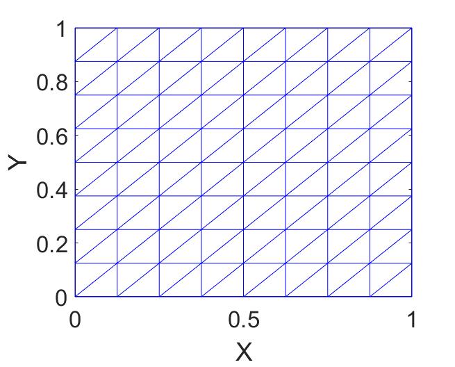Refer to caption — Figure 1. A uniform triangular mesh on the unit square.

We solve the nonlinear FE system (2.3) by the Newton iterative algorithm (4.1)-(4.2) with Taylor-Hood/piecewise linear ( $P2-P1$ ) for $({\boldsymbol{u}},p)$ and the lowest-order first type of Nédélec’s edge element and the lowest-order second type of Nédélec’s edge element, respectively, for the magnetic field ${\boldsymbol{b}}$ . To show the optimal convergence rates, a uniform triangular partition with $M+1$ nodes in each direction is used, see Figure 1 for an illustration. We present in Table 1 numerical results with the lowest-order first type of Nédélec’s edge element for $M=4,8,16,32,64,128$ . From Table 1, we can observe clearly the second-order convergence rate for the velocity ${\boldsymbol{u}}$ in $H^{1}$ -norm and the pressure in $L^{2}$ -norm and the first-order rate for the magnetic field ${\boldsymbol{b}}$ in $H(curl)$ -norm. This confirms our theoretical analysis, while in all previous analysis, only the first-order convergence rate for the velocity was presented. Our numerical results also show that the lower order approximation to the magnetic field does not pollute the accuracy of numerical velocity in $H^{1}$ -norm, although these two physical components are coupled strongly in the MHD system. Moreover, we present in Table 2 numerical results with the lowest-order second type of Nédélec’s edge element approximation to the magnetic field. The accuracy of the lowest-order second type of Nédélec’s edge element approximation is also of the order $O(h)$ in $H(curl)$ -norm. Our numerical results show the same convergence rates as numerical results obtained by the lowest-order first type of Nédélec’s edge element.

Table 1. Errors of Taylor-Hood/lowest-order Nédélec’s edge element of the first type for MHD system (Example 4.1).

$M$	$\\|\nabla({\boldsymbol{u}}-{\boldsymbol{u}}_{h})\\|_{L^{2}}$	Rate	$\\|p-p_{h}\\|_{L^{2}}$	Rate	$\\|{\boldsymbol{b}}-{\boldsymbol{b}}_{h}\\|_{curl}$	Rate	$\\|r-r_{h}\\|_{H^{1}}$
4	1.398e-2		2.774e-2		8.254e-1		1.232e-7
8	2.342e-3	2.58	7.369e-2	1.91	4.274e-1	0.984	5.676e-10
16	4.219e-4	2.47	1.887e-3	1.96	2.093e-1	0.996	2.349e-12
32	8.983e-5	2.23	4.750e-4	1.99	1.047e-1	0.999	3.732e-13
64	2.130e-5	2.08	1.190e-4	2.00	5.237e-2	1.00	1.553e-12
128	5.250e-6	2.02	2.976e-5	2.00	2.168e-2	1.00	6.273e-12

Table 2. Errors of Taylor-Hood/lowest-order Nédélec’s edge element of the second type for MHD system (Example 4.1).

$M$	$\\|\nabla({\boldsymbol{u}}-{\boldsymbol{u}}_{h})\\|_{L^{2}}$	Rate	$\\|p-p_{h}\\|_{L^{2}}$	Rate	$\\|{\boldsymbol{b}}-{\boldsymbol{b}}_{h}\\|_{curl}$	Rate	$\\|r-r_{h}\\|_{H^{1}}$
4	1.137e-2		3.943e-2		8.093e-1		2.007e-4
8	1.829e-3	2.63	1.041e-2	1.92	4.095e-1	0.982	7.128e-6
16	3.669e-4	2.32	2.640e-3	1.98	2.054e-1	0.996	2.331e-7
32	8.484e-5	2.03	6.624e-4	1.99	1.028e-1	0.999	7.415e-9
64	2.075e-5	2.03	1.658e-4	2.00	5.140e-2	1.00	2.334e-10

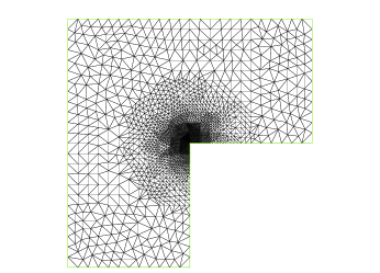
Example 4.2. The second example is to study numerical solution of the MHD system on a non-convex $L$ -shape domain $\Omega:=(-1,1)\times(-1,1)/(0,1]\times[-1,0)$ . The solution of the system may have certain singularity near the re-entrant corner and the regularity of the solution depends upon the interior angles in general. Here we investigate the convergence rates of the method for the problem with a nonsmooth solution. We set $R_{e}=R_{m}=0.1,S=1$ , and choose the source terms and the boundary conditions such that the singular solutions are defined by

	$\displaystyle{\boldsymbol{u}}=\left(\begin{array}[]{cc}\rho^{\lambda}\left((1+\lambda)\sin\theta\phi(\theta)+\cos\theta\phi^{\prime}(\theta)\right)\\ \rho^{\lambda}\left(-(1+\lambda)\cos\theta\phi(\theta)+\sin\theta\phi^{\prime}(\theta)\right)\end{array}\right),\qquad p=\frac{\rho^{\lambda-1}}{1-\lambda}\left((1+\lambda)^{2}\phi^{\prime}(\theta)+\phi^{\prime\prime\prime}(\theta)\right)$		(4.11)
	$\displaystyle{\boldsymbol{b}}=\nabla\left(\rho^{\frac{2}{3}}\sin\left(\frac{2\theta}{3}\right)\right),\qquad\quad r=0$

in the polar coordinate system $(\rho,\theta)$ , where

\displaystyle\phi(\theta)=\sin((1+\lambda)\theta)\frac{\cos(\lambda\omega)}{1+\lambda}-\cos((1+\lambda)\theta)-\sin((1-\lambda)\theta)\frac{\cos(\lambda\omega)}{1-\lambda}+\cos((1-\lambda)\theta)

and the parameters $\lambda=0.54448$ and $\omega=2/3$ . Clearly $({\boldsymbol{u}},p)\in H^{\lambda+1-\epsilon_{0}}(\Omega)\times H^{\lambda-\epsilon_{0}}(\Omega)$ and ${\boldsymbol{b}}\in{\boldsymbol{H}}^{2/3-\epsilon_{0}}(\Omega)$ for any $\epsilon_{0}>0$ . This is a benchmark problem in numerical simulations, which was tested by many authors, $e.g.$ , see [3, 16, 43].

The accuracy of numerical methods usually depends upon the regularity of the exact solution, while theoretical analysis given in this paper is based on the assumption of high regularity. Here we use the same method as described in Table 1. For the solution of the weak regularity as mentioned above, the interpolation error orders on quasi-uniform meshes are

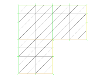
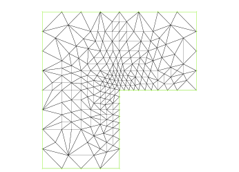
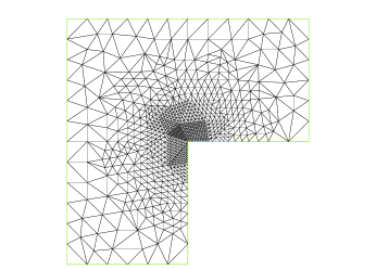
	$\displaystyle\\|\nabla({\boldsymbol{u}}-{\boldsymbol{u}}_{h})\\|_{L^{2}(\Omega)}=O(h^{\lambda-\epsilon_{0}})$
	$\displaystyle\\|{\boldsymbol{b}}-{\boldsymbol{b}}_{h}\\|_{H(curl,\Omega)}=O(h^{2/3-\epsilon_{0}})\,.$

To test the convergence rate, a uniform triangulation is made on the $L$ -shape domain $\Omega$ , see Figure 2 (top left) for a sample mesh, where $M+1$ nodal points locate in the interval $[0,1]$ . We present in Table 3 numerical results obtained by the method with uniform meshes. One can see clearly that the orders of numerical approximations for ${\boldsymbol{u}}$ in $H^{1}$ -norm and for ${\boldsymbol{b}}$ in $H(curl)$ -norm are $0.57$ and $0.63$ , respectively, which are very close to the optimal ones in the sense of interpolation. It has been noted that a local refinement may further improve the convergence rate. Here we test the method with locally refined meshes, although our analysis was given only for a quasi-uniform mesh. We present three non-uniform meshes in Figure 2 with a finer mesh distribution around the re-entrant corner. We present in Table 4 numerical results obtained by the method with these four types of meshes in Figure 2. From Table 4, we can see the second-order convergence rate for the numerical velocity and the first-order convergence rate for the magnetic field approximately. This shows again that the accuracy of the numerical method can be improved dramatically by using such locally refined meshes.

Table 3. Errors of Taylor-Hood/lowest-order Nedelec FEM of the first type for MHD system with the nonsmooth solution in an

L

-shape domain and uniform meshes (Example 4.2).

$M$	$\\|\nabla({\boldsymbol{u}}-{\boldsymbol{u}}_{h})\\|_{L^{2}}$	Rate	$\\|p-p_{h}\\|_{L^{2}}$	Rate	$\\|{\boldsymbol{b}}-{\boldsymbol{b}}_{h}\\|_{curl}$	Rate	$\\|r-r_{h}\\|_{H^{1}}$
4	1.1281		4.775		2.933e-1		1.470e-3
8	7.284e-1	0.815	2.273	1.07	1.742e-1	0.751	2.464e-3
16	4.626e-1	0.655	1.256	0.856	1.117e-1	0.640	1.786e-3
32	3.216e-1	0.525	8.141e-1	0.814	7.279e-2	0.618	1.052e-3
64	2.162e-1	0.573	5.341e-1	0.534	4.703e-2	0.630	4.574e-4

Table 4. Errors of Taylor-Hood/lowest-order Nedelec FEM of the first type for MHD system with the nonsmooth solution in an

L

-shape domain and adaptive meshes (Example 4.2).

Mesh	$\\|\nabla({\boldsymbol{u}}-{\boldsymbol{u}}_{h})\\|_{L^{2}}$	Rate	$\\|p-p_{h}\\|_{L^{2}}$	Rate	$\\|{\boldsymbol{b}}-{\boldsymbol{b}}_{h}\\|_{curl}$	Rate	$\\|r-r_{h}\\|_{H^{1}}$
Mesh I	1.280e-1		4.667e-1		2.912e-1		1.480e-4
Mesh II	6.415e-2	1.07	1.960e-1	1.34	1.591e-1	0.94	3.951e-4
Mesh III	2.017e-2	1.77	6.236e-2	1.75	5.562e-2	1.60	2.771e-5
Mesh IV	7.521e-3	1.85	2.243e-2	1.91	2.715e-2	1.33	2.668e-5

Acknowledgments The author would like to thank the anonymous referees for the careful review and valuable suggestions and comments, which have greatly improved this article.

References

[1] C. Amrouche, C. Bernardi, M. Dauge and V. Girault, Vector potentials in three-dimensional nonsmooth domains, Math. Meth. Appl. Sci., 21 (1998), pp. 823–864.
[2] F. Armero and J.C. Simo, Long-term dissipativity of time-stepping algorithms for an abstract evolution equation with applications to the incompressible MHD and Navier-Stokes equations, Comput. Methods Appl. Mech. Engrg., 131 (1996), pp. 41–90.
[3] S. Badia, R. Codina, and R. Planas, On an unconditionally convergent stabilized finite element approximation of resistive magnetohydrodynamics, J. Comput. Phys., 234 (2013), pp. 399–416.
[4] S.H. Christiansen, H.Z. Munthe-Kaas, and B. Owren, Topics in structure-preserving discretization, Acta Numer., 20 (2011), pp. 1–119.
[5] M. Costabel and M. Dauge, Singularities of electromagnetic fields in polyhedral domains, Arch. Rational Mech. Anal., 151 (2000), pp. 221–276.
[6] M. Dauge, Neumann and mixed problems on curvilinear polyhedra, Integral Equations Oper. Theory, 15 (1992), pp, 227–261.
[7] P.A. Davidson, An introduction to Magnetohydrodynamics, Cambridge University Press, 2001.
[8] Q. Ding, X. Long and S. Mao, Convergence analysis of Crank-Nicolson extrapolated fully discrete scheme for thermally coupled incompressible magnetohydrodynamic system, Applied Numerical Mathematics, 157 (2020), pp. 522–543.
[9] Q. Ding, X. Long and S. Mao, Convergence analysis of a fully discrete finite element method for thermally coupled incompressible MHD problems with temperature-dependent coefficients, ESAIM: M2AN , 56(3) (2022), pp. 969–1005.
[10] X. Dong, Y. He and Y. Zhang, Convergence analysis of three finite element iterative methods for the 2D/3D stationary incompressible magnetohydrodynamics, Comput. Methods Appl. Mech. Engrg., 276 (2014), pp. 287–311.
[11] H. Gao and W. Qiu, A semi-implicit energy conserving finite element method for the dynamical incompressible magnetohydrodynamics equations, Comput. Methods Appl. Mech. Engrg., 346 (2019), pp. 982–1001.
[12] H. Gao and W. Sun, An efficient fully linearized semi-implicit Galerkin-mixed FEM for the dynamical Ginzburg–Landau equations of superconductivity, Journal of Computational Physics, 294 (2015), pp. 329–345.
[13] H. Gao, B. Li and W. Sun, Stability and error estimates of fully discrete Galerkin FEMs for nonlinear thermistor equations in non-convex polygons, Numerische Mathematik, 136(2017), pp.383–409.
[14] J.F. Gerbeau, A stabilized finite element method for the incompressible magnetohydrodynamic equations, Numer. Math., 87 (2000), pp. 83–111.
[15] J.F. Gerbeau, C. Le Bris and T. Leliévre, Mathematical Methods for the Magnetohydrodynamics of Liquid Metals, Numerical Mathematics and Scientific Computation, Oxford University Press, New York (2006).
[16] C. Greif, D. Li, D. Schötzau and X. Wei, A mixed finite element method with exactly divergence-free velocities for incompressible magnetohydrodynamics, Comput. Methods Appl. Mech. Engrg., 199 (2010), pp. 2840–-2855.
[17] M.D. Gunzburger, A.J. Meir and J.P. Peterson, On the existence, uniqueness, and finite element approximation of solutions of the equations of stationary, incompressible magnetohydrodynamics, Math. Comp., 56 (1991), pp. 523–563.
[18] J. Guzmán, D. Leykekhman, J. Rossmann and A.H. Schatz, Hölder estimates for Green’s functions on convex polyhedral domains and their applications to finite element methods, Numer. Math., 112 (2009), pp. 221–243.
[19] Y. He and J. Zou, A priori estimates and optimal finite element approximation of the MHD flow in smooth domains, ESAIM Math. Model. Numer. Anal., 52 (2018), pp.181–206.
[20] Y. He, Unconditional convergence of the Euler semi-implicit scheme for the three-dimensional incompressible MHD equations, IMA Journal of Numerical Analysis, 35(2) (2015), pp. 767–801.
[21] R. Hiptmair, M. Li, S. Mao and W. Zheng, A fully divergence-free finite element method for magnetohydrodynamic equations, Math. Models Methods Appl. Sci., 28 (2018), pp. 659–695.
[22] R. Hiptmair and C. Pagliantini, Splitting-based structure preserving discretizations for magnetohydrodynamics, The SMAI journal of computational mathematics, Volume 4 (2018) , pp. 225–257.
[23] K. Hu, Y. Ma and J. Xu, Stable finite element methods preserving $\nabla\cdot\mathbf{B}=0$ exactly for MHD models, Numer. Math., 135 (2017), pp. 371–396.
[24] K. Hu and J. Xu, Structure-preserving finite element methods for stationary MHD models, Math. Comput., 88 (2019), pp. 553–581.
[25] W.F. Hughes and F.J. Young, The electromagnetics of fluids, Wiley, New York,1966.
[26] D. Jerison and C. Kenig, The inhomogeneous Dirichlet problem in Lipschitz domains, Journal of Functional Analysis, 130 (1995), pp. 161–219.
[27] D. Jin, P.D. Ledger and A.J. Gil, $hp$ -finite element solution of coupled stationary magnetohydrodynamics problems including magnetostrictive effects, Computers & Structures, 164 (2016), pp. 161–180.
[28] J. J. Lee, S.J. Shannon, T. Bui-Thanh and J.N. Shadid. Analysis of an HDG method for linearized incompressible resistive MHD equations, SIAM J. Numer. Anal., 57 (2019), pp.1697–1722.
[29] B. Li, J. Wang and L. Xu, A convergent linearized Lagrange finite element method for the magneto-hydrodynamic equations in two-dimensional nonsmooth and nonconvex domains, SIAM J. Numer. Anal., 58 (2020), pp.430–459.
[30] L. Li and W. Zheng, A robust solver for the finite element approximation of stationary incompressible MHD equations in 3D, J. Comput. Phys., 351 (2017), pp. 254–270.
[31] A.J. Meir and P.G. Schmidt, Analysis and numerical approximation of a stationary MHD flow problem with nonideal boundary, SIAM. J. Numer. Anal., 36 (1999), pp. 1304–1332.
[32] R. Moreau, Magneto-hydrodynamics, Kluwer Academic Publishers, 1990.
[33] U. Müller and L. Büller, Magnetofluiddynamics in Channels and Containers, Springer-Verleg, Berlin, 2001.
[34] P. Monk, Finite Element Methods for Maxwell’s Equations, Oxford University Press, NewYork (2003).
[35] C. Pagliantini, Computational Magnetohydrodynamics with Discrete Differential Forms, Ph.D Thesis (2016), ETH Zürich.
[36] E.G. Phillips and H.C. Elman, A stochastic approach to uncertainty in the equations of MHD kinematics, J. Comput. Phys., 284 (2015), pp. 334–350.
[37] E.G. Phillips, J.N. Shadid, E.C. Cyr, H.C. Elman, and R.P. Pawlowski, Block preconditioners for stable mixed nodal and edge finite element representations of incompressible resistive MHD, SIAM J. Sci. Comput., 38(6) 2016, pp. B1009–B1031.
[38] W. Qiu and K. Shi, A mixed DG method and an HDG method for incompressible magnetohydrodynamics, IMA Journal of Numerical Analysis, 40(2) (2020), pp. 1356–1389.
[39] A. Schneebeli and D. Schötzau, Mixed finite elements for incompressible magneto-hydrodynamics, C. R. Acad. Sci. Paris, Ser. I, 337(1) (2003) , pp. 71–74.
[40] D. Schötzau, Mixed finite element methods for stationary incompressible magnetohydrodynamics, Numer. Math., 96 (2004), pp. 315–341.
[41] M. Wathen and Chen Greif, A scalable approximate inverse block preconditioner for an incompressible magnetohydrodynamics model problem, SIAM J. Sci. Comput., 42(1) (2020), pp. B57–B79.
[42] M. Wathen, Chen Greif, and D. Schötzau, Preconditioners for mixed finite element discretizations of incompressible MHD equations, SIAM J. Sci. Comput., 39(6) (2017), pp. A2993–A3013.
[43] G. Zhang, Y. He and D. Yang, Analysis of coupling iterations based on the finite element method for stationary magnetohydrodynamics on a general domain, Computers $\&$ Mathematics with Applications, 68(7) (2014), pp. 770–788

	$\displaystyle\\|{\boldsymbol{b}}\\|_{W^{1,d^{+}}(\Omega)}+\\|\nabla\times{\boldsymbol{b}}\\|_{W^{1,d^{+}}(\Omega)}+\\|{\boldsymbol{u}}\\|_{H^{l+1}(\Omega)}$	$\displaystyle+\\|p\\|_{H^{l}(\Omega)}+\\|{\boldsymbol{b}}\\|_{H^{k}(\Omega)}$
		$\displaystyle+\\|\nabla\times{\boldsymbol{b}}\\|_{H^{k}(\Omega)}+\\|r\\|_{H^{k+1}(\Omega)}\leq K.$		(2.16)

	$\displaystyle\\|\nabla\times(\widehat{{\boldsymbol{b}}}_{h}-{\boldsymbol{b}})\\|_{L^{2}(\Omega)}$	$\displaystyle+\\|\widehat{{\boldsymbol{b}}}_{h}-{\boldsymbol{b}}\\|_{L^{2}(\Omega)}+\\|\nabla(\widehat{r}_{h}-r)\\|_{L^{2}(\Omega)}$
		$\displaystyle\leq Ch^{\min(k,s)}\left(\\|{\boldsymbol{b}}\\|_{H^{s}(\Omega)}+\\|\nabla\times{\boldsymbol{b}}\\|_{H^{s}(\Omega)}+\\|r\\|_{H^{s+1}(\Omega)}\right)$		(3.6)

	$\displaystyle\\|{\boldsymbol{b}}-\Pi_{h}^{\text{curl}}{\boldsymbol{b}}\\|_{L^{3}(\Omega)}\leq$	$\displaystyle Ch^{\min(k,s)}\\|{\boldsymbol{b}}\\|_{W^{s,3}(\Omega)},$
	$\displaystyle\\|{\boldsymbol{b}}-\Pi_{h}^{\text{curl}}{\boldsymbol{b}}\\|_{H(\text{curl},\Omega)}\leq$	$\displaystyle Ch^{\min(k,s)}\left(\\|{\boldsymbol{b}}\\|_{H^{s}(\Omega)}+\\|\nabla\times{\boldsymbol{b}}\\|_{H^{s}(\Omega)}\right).$

	$\displaystyle\\|{\boldsymbol{b}}-\tilde{{\boldsymbol{b}}}_{h}\\|_{H^{-1}(\Omega)}\leq$	$\displaystyle CC_{3}h\left(\\|{\boldsymbol{b}}-\tilde{{\boldsymbol{b}}}_{h}\\|_{H(\text{curl},\Omega)}+\\|\nabla(r-\tilde{r}_{h})\\|_{L^{2}(\Omega)}\right)$		(3.21)
	$\displaystyle\leq$	$\displaystyle CC_{3}h^{k+1}\left(\\|{\boldsymbol{b}}\\|_{H^{k}(\Omega)}+\\|\nabla\times{\boldsymbol{b}}\\|_{H^{k}(\Omega)}+\\|r\\|_{H^{k+1}(\Omega)}\right).$

	$\displaystyle\|c_{1}({\boldsymbol{b}}_{h};\xi_{{\boldsymbol{u}}},e_{{\boldsymbol{b}}})\|$	$\displaystyle=\|c_{1}(\tilde{\boldsymbol{b}}_{h};\xi_{{\boldsymbol{u}}},e_{{\boldsymbol{b}}})-c_{1}(e_{\boldsymbol{b}};\xi_{{\boldsymbol{u}}},e_{{\boldsymbol{b}}})\|$
		$\displaystyle\leq C(\\|\nabla\times e_{{\boldsymbol{b}}}\\|_{L^{2}(\Omega)}\\|\xi_{{\boldsymbol{u}}}\\|_{L^{6}(\Omega)}+\\|\tilde{\boldsymbol{b}}_{h}\\|_{L^{\infty}(\Omega)}\\|\xi_{{\boldsymbol{u}}}\\|_{L^{2}(\Omega)})\\|e_{{\boldsymbol{b}}}\\|_{H(\text{curl},\Omega)}$
		$\displaystyle\leq\epsilon\\|e_{{\boldsymbol{b}}}\\|_{H(\text{curl},\Omega)}^{2}+C_{K}h^{2l+2}$