New Highly Efficient High-Breakdown Estimator of Multivariate Scatter and Location for Elliptical Distributions
Abstract
High-breakdown-point estimators of multivariate location and shape matrices, such as the MM-estimator with smooth hard rejection and the Rocke S-estimator, are generally designed to have high efficiency at the Gaussian distribution. However, many phenomena are non-Gaussian, and these estimators can therefore have poor efficiency. This paper proposes a new tunable S-estimator, termed the S-q estimator, for the general class of symmetric elliptical distributions, a class containing many common families such as the multivariate Gaussian, t-, Cauchy, Laplace, hyperbolic, and normal inverse Gaussian distributions. Across this class, the S-q estimator is shown to generally provide higher maximum efficiency than other leading high-breakdown estimators while maintaining the maximum breakdown point. Furthermore, its robustness is demonstrated to be on par with these leading estimators while also being more stable with respect to initial conditions. From a practical viewpoint, these properties make the S-q broadly applicable for practitioners. This is demonstrated with an example application—the minimum-variance optimal allocation of financial portfolio investments.
keywords:
Covariance matrix estimation , Robust estimation , S-estimator , S-q estimator , Shape matrix estimation[inst1]organization=Bradley Department of Electrical and Computer Engineering
Virginia Polytechnic Institute and State University,addressline=
7054 Haycock Rd,
city=Falls Church,
postcode=22043,
state=VA,
country=USA
1 Introduction
Huber (1964) introduced what is the most common class of estimators, M-estimators. Although originally applied to the location case, Maronna (1976) expanded the definition to include multivariate location and scatter. After the sample median, perhaps the most common robust M-estimators are those using the general rho functions such as the Huber or Tukey bisquare functions.
However, the drawback of using general rho functions is that they have limited efficiency when applied to parameter estimation of nonideal probability distributions. To address this, various M-estimator approaches have been taken to iteratively reweight maximum likelihood estimator (MLE) weights based on the estimated probability density function (PDF) (e.g., Windham, 1995; Basu et al., 1998; Choi and Hall, 2000; Ferrari and Yang, 2010).
Even with these improvements, multivariate M-estimators inherently have limited robustness. For example, Maronna (1976) showed that the upper-bound on the breakdown point for -dimensional M-estimators is , which converges to zero with large . To combat this weakness, Rousseeuw and Yohai (1984) introduced regression S-estimators, which Davies (1987) expanded to multivariate location and scatter. Davies also showed that the asymptotic breakdown point of S-estimators can be set to 1/2, which is the theoretical maximum of any equivariant estimator.
In practical scenarios however, estimators may have large bias at considerably lower contamination levels than the breakdown point. For many years, the Tukey bisquare was the standard rho function for S-estimators (for example, see Lopuhaä, 1989; Rocke, 1996). However, in the context of multivariate S-estimators, the bisquare is not tunable, so its robustness falls off with increasing . For this reason, Rocke (1996) introduced the tunable biflat and translated biweight rho functions. Maronna et al. (2006, sec. 6.4.4) slightly modified the biflat, proposing the Rocke rho function. The Rocke S-estimator (shortened here to S-Rocke) is currently the recommended high-breakdown estimator for large dimensions (Maronna and Yohai, 2017; Maronna et al., 2019, sec. 6.10). The recommended estimator for lower dimensions is the MM-estimator with the smoothed hard rejection function (MM-SHR).
There are two major shortcomings of the S-Rocke estimator that will be discussed in this paper. Firstly, it has low efficiency for small dimension, . Although this is an inherent disadvantage of all S-estimators, it is exceptionally acute for the S-Rocke. Secondly, the S-Rocke has poor efficiency for most common non-Gaussian distributions. This is a common problem for general-purpose estimators such as the Rocke and bisquare S-estimators, the MM-SHR, and the Huber and bisquare M-estimators. Examples of common phenomena that are frequently modeled by non-Gaussian distributions include stock returns, radar sea clutter, and speech signals, which approximately follow generalized hyperbolic (Konlack Socgnia and Wilcox, 2014), K- (Ward et al., 1990), and Laplace distributions (Gazor and Zhang, 2003), respectively.
This paper proposes and explores a new subclass of tunable, maximum-breakdown-point S-estimators that is applicable across common continuous elliptical distributions. This estimator, named the S-q estimator, uses a density-based reweighting to attain generally higher maximum efficiency across the elliptical class as compared to the S-Rocke and MM-SHR estimators. These estimators are compared from the viewpoints of statistical and computational efficiency, robustness, and stability.
Although the focus on elliptical distributions sounds limiting, as discussed in the next section, most common continuous multivariate distributions—such as the Gaussian, t-, Laplace, and hyperbolic distributions—fall into this class. As Frahm (2009) discussed, this assumption is “fundamental in multivariate analysis.”
This paper is organized as follows. Section 2 defines the new estimator and provides its functions for the most common elliptical distributions. Basic properties related to the consistency of the S-q estimator are summarized in Section 3. Section 4 provides the asymptotic distribution of the S-q estimator and compares the maximum achievable efficiencies of the S-q, S-Rocke, and MM-SHR estimators. In Section 5, the finite-sample breakdown point of the S-q is discussed, the theoretical influence functions of the estimators are compared, and the empirical finite-sample robustness of the estimators are briefly explored. Section 6 assesses two computational aspects of the estimators: computational efficiency, and stability with respect to initial estimates. A real-world example in Section 7 demonstrates the application of the estimators for the minimum-variance optimal allocation of financial portfolio investments. Finally, conclusions are summarized in Section 8.
2 Defining the S-q Estimator
This section builds the definition of the proposed S-q estimator. First, the elliptical class of distributions is reviewed. The multivariate S-estimator definition is then summarized, and finally, the S-q is defined.
2.1 Elliptical Distributions
The elliptical distribution is a general class of multivariate probability distributions encompassing many familiar subclasses such as the symmetric Gaussian, t-, Cauchy, Laplace, hyperbolic, variance gamma, and normal inverse Gaussian distributions. Table 1 summarizes the most common elliptical distributions (Fang et al., 1990, p. 69; Deng and Yao, 2018).
| Distribution Name | Generating Function, |
|---|---|
| {Range of Parameters} | |
| Kotz type | |
| Gaussian | |
| (Kotz type with ) | |
| Pearson type II | , |
| Pearson type VII | |
| t | |
| (Pearson VII with ) | |
| Cauchy | |
| (t with ) | |
| Generalized hyperbolic | |
| Variance gamma | |
| (Gen. hyperbolic with ) | |
| Laplace | |
| (Variance gamma with ) | |
| Multivariate hyperbolic | |
| (Gen. hyperbolic with ) | |
| Hyperbolic with univariate marginals | |
| (Gen. hyperbolic with ) | |
| Normal inverse Gaussian | |
| (Gen. hyperbolic with ) |
Symmetric elliptical distributions are defined as being a function of the squared Mahalanobis distance,111Some texts define the Mahalanobis distance with the mean and covariance, but this more restrictive definition excludes thick-tailed distributions where these do not exist, such as Cauchy distributions. , where , the location , and the positive definite symmetric () scatter . When the PDF is defined, it has the form for some generating function , and where is a constant that ensures integrates to one. Table 1 lists common generating functions. When the covariance exists, it is proportional to the scatter matrix, . The corresponding shape matrix is commonly defined as
| (1) |
The PDF of is given by (Kelker, 1970)
| (2) |
where . Hereafter, all densities, refer to the density of in (2), so the subscript will be omitted. It is also generally assumed that
2.2 S-Estimators
Given a set of -dimensional samples, , S-estimators of location and shape are defined as (Maronna et al., 2006, Sec. 6.4.2)
| (3) | ||||||
| subject to | ||||||
for some scalar rho function, . A proper S-estimator rho function should be a continuously differentiable, nondecreasing function in with , and where there is a point such that for . For simplicity, and without loss of generality, the rho functions will be normalized so . The parameter is a scalar that affects the efficiency (see Section 4) and robustness of the estimator. The purpose of S-estimators is to achieve high robustness, so they are usually configured with which achieves the maximum theoretical breakdown point that any affine equivariant estimator may have (see Section 5.1). To understand the derivation of the proposed estimator in the next section, note that in the constraint is an M-estimator of the scale of Local solutions of (3) can be found iteratively using the weighted sums and where the weight function and where is re-normalized with each iteration. For the empirical results in this paper, the estimators will all be solved using this weighted-sum algorithm.
To estimate the scatter metrix, a separate estimator of can then be used to scale using (1). Maronna et al. (2006, p. 186) discussed a simple estimator to scale to . When is normally distributed, has a chi-squared distribution with degrees of freedom. Therefore, they suggested using , where is the 50th percentile of the chi-squared distribution. For the general case of elliptical distributions, we propose extending this to
where is the distribution function corresponding to (2), and therefore is the 50th percentile of the distribution.
For the location and shape matrices, the S-estimator formulation in (3) is equivalent to the alternative one given by
| (4) | ||||||
| subject to |
which requires that be defined such that for a consistent estimator of at an assumed elliptical distribution (Rocke, 1996). While the first formulation is better for understanding the derivation of the proposed S-q estimator, this second formulation is better for defining and understanding its properties (for example, see Lopuhaä, 1989). The scale parameters in the two formulations are related asymptotically by at the assumed distribution.
The two most common multivariate S-estimators are the bisquare and Rocke (Maronna et al., 2019, sec. 6.4.2, 6.4.4). The S-bisquare is given by and which does not have a tuning parameter to control efficiency and robustness. The S-Rocke is given by
where the parameter tunes the estimator’s efficiency and robustness. The Rocke’s maximum efficiency is generally limited at , which is extremely restricting for small . Both and are generic functions that do not depend on the underlying distribution. In the following section, an alternative S-estimator is defined that accounts for the underlying distribution and that generally has better performance across the most common elliptical distributions. It also does not have the same inherent restrictions for small as
2.3 Elliptical Density-Based S-q Estimator
The rho function corresponding to the maximum likelihood estimator, of the scale of or equivalently is We propose weighting this by the power transform of the density, where the scalar controls the estimator robustness, with corresponding to the maximum likelihood function, and with decreasing increasing the estimator robustness. In most cases, this rho function is not monotone, as required by S-estimators, so it is denoted with a tilde. This rho function is equivalent to the M-Lq and other M-estimators proposed, for example, by Windham (1995); Basu et al. (1998); Choi and Hall (2000); and Ferrari and Yang (2010). However, in this particular case of estimating the scale of the squared Mahalanobis distance of an elliptically distributed random vector, the density and rho function do not need to be regenerated with each numerical iteration, based on the estimates and Substituting the PDF from (2),
| (5) |
where and . Taking the derivative of , the corresponding weight function is given by
| (6) |
For simplicity, when , the scalar can be dropped from the calculation of and in (5) and (6). When is only positive over a finite domain (e.g. Pearson Type II distribution), then we define and to be zero outside this domain.
For the common elliptical distributions listed in Table 1, is monotone in its central region between its global extrema when using appropriate values for (defined below). The first extremum is the minimum, which we label point , and the second is the maximum, labeled . The distance between and varies monotonically with respect to . We use this to define a tunable, double-hard-rejection S-estimator rho function. The value of is held constant between zero and at value which hard rejects inliers, and the value of is held constant above at value which hard rejects outliers. The resulting monotonic function is then scaled and shifted so it ranges from zero to one. This defines the S-q estimator.
Definition 1.
Assuming is twice continuously differentiable over its region of support and has one or two zeros in for , the S-q estimator is the S-estimator with the rho function given by
| (7) |
where . The S-q estimator of Type I is the case with one zero (i.e. ), and the Type II S-q estimator is the case with two zeros.
For most distributions, or at , is not bounded. Therefore, we do not scale or shift in this case, and is not a proper S-estimator rho function. However, when and , the MLE of the scale of is obtained. The S-q weight function is the derivative of and is given by
| (8) |
Table 2 lists expressions for the inlier rejection point, and the outlier rejection point, , for the common elliptical distributions in Table 1. For most of these distributions, the equation is quadratic, which provides a closed-form solution for the values of and .
| Distribution | Inlier Rejection Point and Outlier Rejection Point | |
|---|---|---|
| Kotz type | ||
| Gaussian | ||
| Pearson type II | ||
| Pearson type VII | ||
| Generalized hyperbolic | ||
The asymptotic rejection probability (ARP) is defined as (Rocke, 1996). Table 2 can be used to determine from a desired ARP using . However, since is very tapered (i.e. applying little weight to values just below ), practitioners may choose alternative approaches to tuning that allow for higher estimator efficiencies. For example, the approach used in this paper as well as in Maronna and Yohai (2017) is to tune the estimators to a desired expected efficiency, which is defined in the next section.
The general definition in (7) specifies that . In a few particular cases, however, there are some minor restrictions on (when ) in order to ensure that and are in the support of . Table 3 lists these restrictions.
| Distribution | Valid Range of |
|---|---|
| Kotz type | unless , then |
| Gaussian | |
| Pearson type II | or |
| Pearson type VII | |
| Generalized hyperbolic* | unless and , then |
| *Empirically inferred. Computational precision restricts approximately. | |
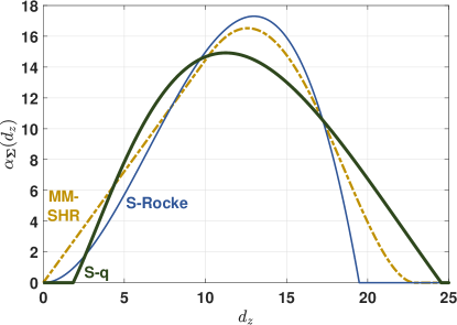
Figure 1 illustrates examples of the S-q functions , , and for the five-dimensional Gaussian (S-q Type II) and Laplace (S-q Type I) distributions and for various values of . As is decreased, the region of positive weights (area between points and ) narrows, corresponding to increased robustness. The PDF is also plotted, illustrating how roughly follows in the central region.
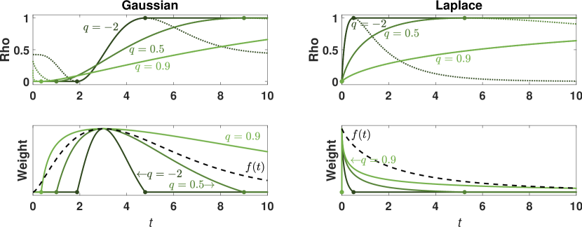
Figure 2 compares the S-q asymptotic weights with those of the MM-SHR, S-Rocke, S-bisquare, and maximum likelihood estimators, and with the corresponding PDF. The underlying model is a 10-dimensional standard Gaussian distribution. The MM-SHR and S-q estimators have been tuned to 80% asymptotic efficiency relative to the MLE. The S-Rocke estimator is tuned to its maximum efficiency, which is 77% in this instance. The estimators have been set to the maximum breakdown point, with which results in the shifts of the peaks of the weight curves relative to the PDF.
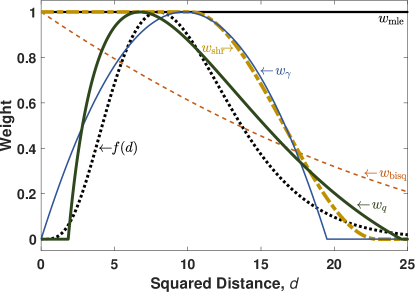
From the figure, it is clear that the Gaussian MLE (i.e. sample estimator) gives uniform weight to all samples, no matter how improbable. The S-Rocke has a quadratic weight function, which is a hard cutoff that cannot capture the tails of . The SHR weight function is cubic, and its shape better captures the shape of the right-half of the PDF. However, the SHR function is designed to approximate a step function, which is poorly suited for many distributions (c.f. in Figure 2 with the Laplace in Figure 1). Only the S-q weight function follows the general shape of the PDF—giving less weight to less probable observations.
3 Consistency Properties of the S-q Estimator
As an S-estimator, the S-q estimator inherits properties from its parent class, such as affine equivariance. This section briefly summarizes properties related to its consistency. For more detailed discussion on these, see (Davies, 1987). Here, we use the alternative S-estimator formulation given by (4) under the assumptions (A1) that
| (A1) | |||
| is non-increasing, and | |||
| and have common point(s) of decrease. |
Theorem 1 (Uniqueness).
Given (A1), minimizing subject to
has a unique solution
Proof.
See (Davies, 1987, Th. 1). ∎
Theorem 2 (Existence).
Given (A1) and then the S-q estimator has at least one solution with probability one.
Proof.
See (Davies, 1987, Th. 2). ∎
Theorem 3 (Consistency).
Given (A1), and then
Proof.
See (Davies, 1987, Th. 3). ∎
4 Asymptotic Distribution and Relative Efficiencies
In this section, the asymptotic distribution of the S-q estimator is provided. From this, measures of efficiency are then defined. Finally, the efficiency of the S-q estimator is compared with leading high-breakdown point estimators.
4.1 Asymptotic Distribution
For the asymptotic distribution of the S-q estimate, we continue to use the alternative S-estimator formulation given by (4). Lopuhaä (1997) derived the distribution of S-estimators with assumptions appropriate for the S-q estimator, that is
| (A2) | is decreasing with . |
Here, we use the following notation. The matrix is the identity matrix, is the commutation matrix, is the Kronecker product operator, and the operator stacks the columns if into a column vector.
Theorem 4 (Asymptotic distribution).
Given (A1) and (A2), the asymptotic distribution of the S-q estimate of is given by , with . The vector where
| (9) |
with and . The matrix where
| (10) |
with and , where and
Proof.
See (Lopuhaä, 1997, Corollary 2). ∎
Frahm (2009) derived the asymptotic distribution of shape matrix estimates for affine equivariant estimators. This enables us to state the asymptotic distribution of the S-q shape estimate, which is applicable using either S-estimator formulation, (3) or (4).
Theorem 5 (Shape asymptotic distribution).
Given (A1) and (A2), the asymptotic distribution of the S-q estimate of shape is given by where
| (11) |
with defined as in Theorem 4.
Proof.
See (Frahm, 2009, Corollary 1). ∎
4.2 Measures of Efficiency
The asymptotic efficiency of an estimator, at an assumed distribution, is defined as the ratio of the asymptotic variance of the maximum likelihood estimate to the variance of the estimator under consideration. For multivariate estimation, this definition of efficiency is of large dimension— for location and for shape and scatter. However, for affine equivariant estimation of location and scatter of elliptical distributions, the covariance of the estimate depends only on a scalar. Specifically, (9), (10), and (11) are general, with only the scalars (Bilodeau and Brenner, 1999), and and (Tyler, 1982) depending on the estimator and the generating function . Therefore, the asymptotic efficiency of the estimate can be alternatively defined as
and the asymptotic efficiency of the estimate can alternatively be defined as
| (12) |
It is common to define asymptotic efficiency this way (for example, see Tyler, 1983; Frahm, 2009).
Comparing the S-q estimator’s efficiency to another estimator can likewise be achieved analytically using, for example, for the S-Rocke estimator, which when the quotient is greater than one, indicates that the S-q has higher asymptotic efficiency than the S-Rocke estimator. For other S-estimators, the asymptotic distribution parameters and are calculated the same as in Theorems 4 and 5 but using their respective weight functions. MM-estimators have the same asymptotic variance and influence function as S-estimators (Rousseeuw and Hubert, 2013). For MM-estimators, however, is effectively the tuning parameter, and it can be set accordingly.
In general, finite-sample performance measures are difficult to derive analytically. Instead, it is common to characterize finite-sample performance by empirically characterizing the behavior of metrics derived from the Kullback-Leibler divergence between the estimated and true distribution (for example, see Huang et al., 2006; Ferrari and Yang, 2010). For t-distributions, which includes the Gaussian distribution, the Kullback-Leibler divergence between and is given by (Abusev, 2015)
Following Maronna and Yohai (2017), we then define the joint location and scatter finite-sample relative efficiency as
where and are the location and scatter matrices corresponding to the maximum likelihood estimate, and where the expectation is calculated empirically using the sample mean over Monte Carlo trials. The location and the scatter finite-sample relative efficiencies are then respectively defined as and Likewise, we define the shape matrix finite-sample relative efficiency as
| (13) |
4.3 Comparison of Estimator Efficiency
Any estimator must provide a good estimate in the absence of contamination and when tuned to its maximum efficiency. This section compares the maximum achievable efficiencies of the S-q, S-Rocke, and MM-SHR estimators when set to their maximum breakdown point. The results below cover large swaths of the most common elliptical families in Table 1 for a moderate dimension of These swaths were specifically chosen to cover everyday distributions: Gaussian, Cauchy, Laplace, hyperbolic, and normal inverse Gaussian distributions.
Robust scatter matrix estimation is generally “more difficult” than the estimation of location (Maronna et al., 2019), and as Maronna and Yohai (2017) demonstrated, divergence and efficiency metrics for scatter matrix estimators are generally much worse than for the corresponding estimators of location. Likewise, due to the high dimensionality of the estimate, the underlying shape matrix is the most difficult part of estimating the scatter matrix. Additionally, many practical applications such as multivariate regression, principal components analysis, linear discriminant analysis, and canonical correlation analysis only require the shape matrix, and not the full scatter or covariance matrices (Frahm, 2009). Therefore, unless otherwise noted, the performance results in this paper are for the shape matrix, with metrics given by (12), (13), and
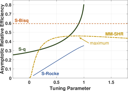
The maximum efficiencies of the S-q and S-Rocke generally occur when their parameters and are set to one—although the maximum breakdown point of the S-q is only achieved when . However, the maximum efficiency of the MM-SHR must be determined by a search as depicted in Figure 3, which plots, as an example, asymptotic efficiency versus tuning parameter for the estimators for the 20-dimensional Cauchy distribution. At the limit, as the MM-SHR parameter is increased toward infinity, all samples receive equal weight, which is the MLE for the Gaussian distribution, but not for distributions such as the Cauchy. In general, for each tunable estimator, its efficiency decreases while its robustness increases as its parameter is decreased. At the lower limit of its parameter, its weight function is a delta function that may reject all the samples and may result in zero efficiency. At this point, the robustness is high, but the weighted-sum solution depends entirely on the initial estimates and
It should be noted that although generally of high efficiency, the S-q estimate at its limit with is not necessarily the maximum likelihood estimate for location and scatter. The MLE weight function for location and scatter is given by (Tyler, 1982)
| (14) |
whereas at (8) gives
| (15) |
Theorem 6 (Relation to MLE efficiency).
Assuming the asymptotic S-q estimate with is the maximum likelihood estimate for the location and scatter matrices for distributions where
| (16) |
for some value Therefore, the S-q estimator can asymptotically achieve the Cramér–Rao lower bound for these distributions.
Proof.
Remark 1.
Remark 2.
If is finite, and then both the Cramér–Rao lower bound (maximum efficiency) and the maximum breakdown point can occur in the limit as (see Corollary 1 in the next section).
An example family that satisfies this theorem is the Kotz type with parameter Note, however, that so high breakdown cannot be achieved simultaneously. This is illustrated in Figure 4, which provides the estimators’ maximum achievable asymptotic shape efficiencies for the Kotz type distribution with parameters and as a function of parameter . In this example, the S-q efficiency is plotted for its maximum absolute efficiency with and for it approximate maximum high-breakdown efficiency with As seen in the figure, the high cost of high-breakdown is particularly acute for large
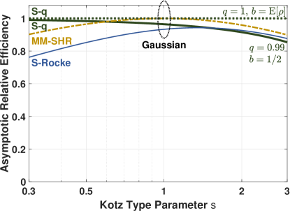
The remainder of this paper will focus on maximum efficiency at the maximum breakdown point. Figure 4 also provides the S-Rocke and MM-SHR estimator’s maximum efficiencies at their maximum breakdown points. The MM-SHR efficiency peaks at which is expected since this is the Gaussian distribution, and the S-Rocke efficiency peaks just above this point. Their efficiencies fall off precipitously for larger and smaller values of The efficiency of the S-q, conversely, increases toward unity for smaller
The estimators’ maximum achievable asymptotic efficiencies for the t-distribution as a function of the distribution parameter, , are plotted on the left of Figure 5. When , the t-distribution corresponds to a Cauchy distribution, and when it corresponds to the Gaussian distribution. The S-q estimator offers the highest efficiency of the three estimators for thicker tails.
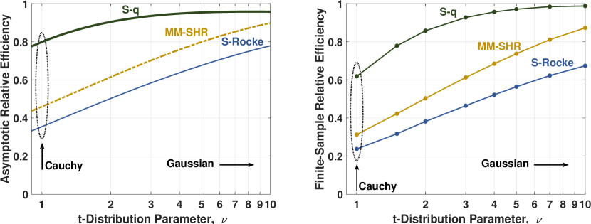
The maximum achievable small-sample relative efficiencies using are plotted on the right of Figure 5. The initial estimates were made using the Peña and Prieto (2007) kurtosis plus specific directions (KSD) estimator as recommended and provided by Maronna and Yohai (2017). Comparing these finite-sample results with the asymptotic ones on the left, it is seen that the relative results are similar. This general similarity implies that the relative performance of the asymptotic efficiencies can often be a good surrogate for the relative performance of the finite-sample efficiencies when there is no closed-form expression for the divergence in (13).
The estimators’ maximum achievable asymptotic efficiencies for the variance gamma distribution with are plotted as a function of parameter on the left of Figure 6. The plots highlight the Laplace and multivariate hyperbolic distributions. The S-q exhibits good performance for the hyperbolic and remarkably good performance for the Laplace.
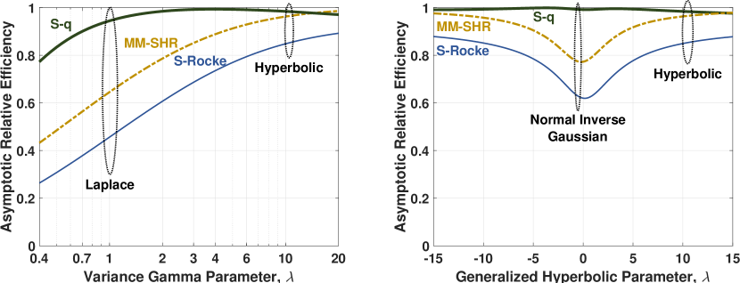
The estimators’ maximum achievable asymptotic efficiencies for the generalized hyperbolic distribution with and are plotted as a function of parameter on the right of Figure 6. The plots highlight the normal inverse Gaussian and hyperbolic distributions. The S-q again exhibits good performance for the hyperbolic, and it exhibits remarkably good performance for the normal inverse Gaussian.
5 Robustness Analysis
The robustness of the S-q estimator is now explored. First, the breakdown point is provided. The influence function is then explored. Finally, finite-sample simulation results are provided to further illustrate the robustness of the high-breakdown estimators.
5.1 Breakdown Point
The finite-sample breakdown point of a multivariate estimator of location or scatter is defined as the fraction of the samples, that can be set to either drive or drive an eigenvalue of to either zero or infinity. Unlike multivariate M-estimators, which only achieve an asymptotic breakdown point of (Maronna, 1976), S-estimators are able to achieve the maximum possible finite-sample breakdown point that any affine equivariant estimator may have (Davies, 1987, Th. 6). For the following theorem, the term samples in general position means that no more than samples are contained in any hyperplane of dimension less than .
Theorem 7 (Finite-sample breakdown point).
Assuming (A1) and when samples are in general position and the breakdown point of the S-q estimator is
Proof.
Corollary 1.
The maximum breakdown point is which is achieved when Asymptotically, this is at
5.2 Influence Function
The influence function (IF) of an estimator characterizes its sensitivity to an infinitesimal point contamination at standardized by the mass of the contamination, The influence function for estimator at the nominal distribution , is defined as
where is the proportion of samples that are a point-mass, located at
Theorem 8 (Influence function).
Assuming (A1) and (A2), the influence functions of for the S-q estimates of and are given by
| (17) |
where and and where the scalars , , and were defined in Theorem 4.
By definition of S-estimators with normalized rho function, the magnitude of first term of (17) is clearly bounded to no more than Therefore, to compare the influence functions of the S-q, S-Rocke, and MM-SHR estimators, we focus on the second term. From this term, define for each estimator. Figure 7 plots at the 10-dimensional Gaussian distribution for the estimators as depicted in Figure 2.
By definition, all highly-robust estimators have bounded influence functions, and for the three estimators considered here, their influence functions are continuous. This means that small amounts of contamination have limited effects on their estimates. The gross-error sensitivity of an estimator is the maximum of and in this example, the S-q demonstrates a lower gross-error sensitivity than the S-Rocke and MM-SHR estimators. By its definition, the MM-SHR has a inlier rejection point of zero, meaning inliers can negatively influence its estimates. However, proper Type II S-q functions have positive inlier rejection points, which provide robustness against inliers.
Relative to the S-Rocke and MM-SHR estimators, the S-q often has larger outlier rejection points. This is the cost of its generally higher efficiency and ability to reject inliers. However, due to its continuity, the influence near this point is still greatly attenuated.
5.3 Finite-Sample Robustness
To empirically compare the finite-sample robustness of the estimators, we employed the simulation method used by Maronna and Yohai (2017) and plot the shape matrix divergence, , versus shift contamination value . For a contamination proportion , the first element of each of the contaminated samples was replaced with the value , that is . The initial estimates of the weighted algorithm were determined with the KSD estimator. Figure 8 provides divergence plots for normally distributed data with contamination, for dimensions and , and for sample sizes and . For the cases where , the estimators were tuned to 90% uncontaminated relative efficiency. When , the S-Rocke has poor maximum efficiency, so the estimators were tuned to match the maximum S-Rocke efficiency.
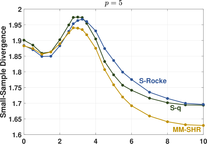
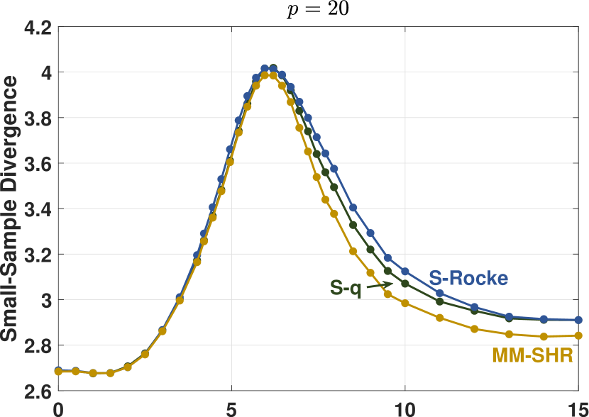
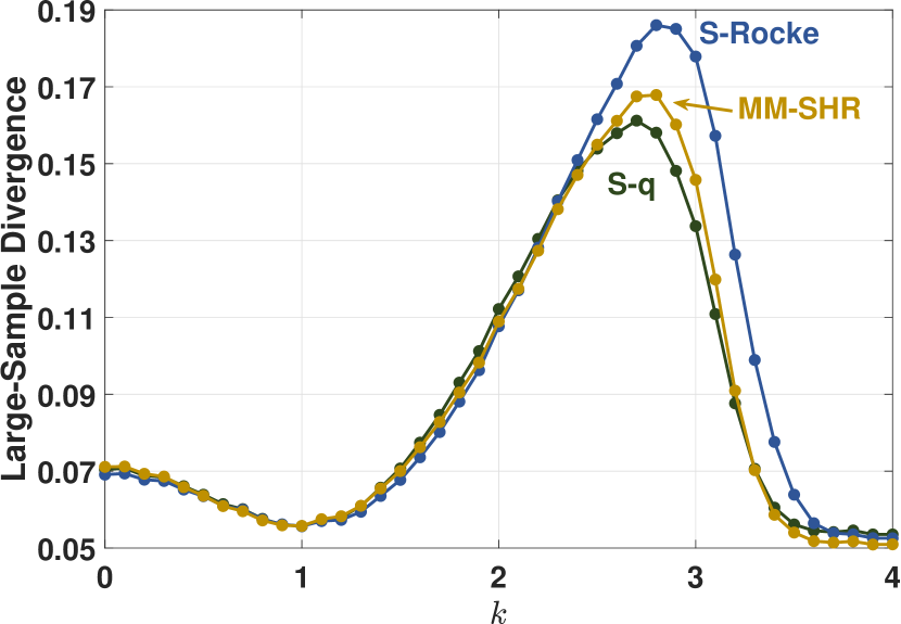
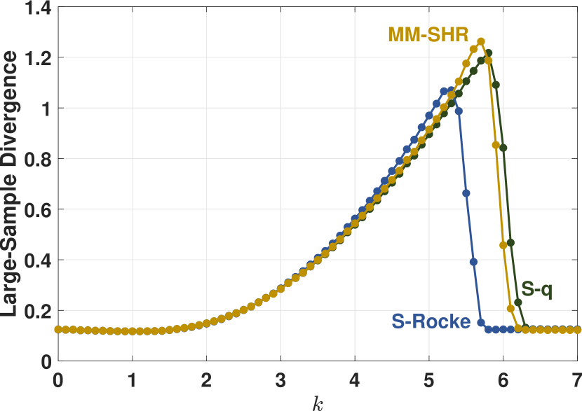
These plots show that the robustness of the S-q is on par with the other two estimators. Consistent with the results in Maronna and Yohai (2017), the relative worst-case performance of the estimators vary by such factors as dimension, sample size, and contamination percentage. For example, the S-q performs the best here for , , but the MM-SHR is the best for , .
6 Computational Aspects
This section explores computational aspects of the S-q and other high-breakdown estimators when using their weighted-sum algorithms. The estimators’ stabilities are first assessed by comparing their sensitivities to the initial estimates, and The computational efficiency is then evaluated by comparing the computational convergence rates of the estimators.
6.1 Stability
The primary criticism of high-breakdown estimators is that their solutions are highly sensitive to the initial estimates and due to the non-convexity of their objective functions. The S-q estimator helps mitigate this with a generally wider weight function (see for example Figure 2). To demonstrate that the S-q is more stable with respect to the initial estimates, Gaussian Monte Carlo simulation trials were run where for each trial, was estimated twice for each estimator using different initializations. For the first estimate, was set to the MLE using all samples before contamination. For the second estimate, was set to the MLE using just 25% of the samples before contamination, resulting in a larger expected variance of The sample mean of the divergence between the two final estimates, was then calculated. The same values of and were used as in the Section 5.3 simulations. The contamination method was also the same, and the value of was set to the worst-case value for that estimator and for the values of and (see Figure 8).
The results are presented in the center of Table 4. It is seen that the S-q estimator was consistently the most stable of the three estimators, and the MM-SHR was generally the most sensitive. For the near-asymptotic cases, the S-q exhibited no measurable differences between the two estimates, unlike the MM-SHR. Like the S-q, the S-Rocke had no measurable differences between the two estimates for the uncontaminated near-asymptotic cases, but under contamination, its mean divergence was roughly on par with the MM-SHR.
| Dim. | Samples | Contam. | Mean Divergence | Median No. of Iterations | |||||
|---|---|---|---|---|---|---|---|---|---|
| S-q | S-Rocke | MM-SHR | S-q | S-Rocke | MM-SHR | ||||
| 5 | 0% | 0 | 0 | 8e-5 | 13 | 14 | 14 | ||
| 5 | 10% | 0 | 7e-4 | 5e-4 | 14 | 15 | 15 | ||
| 20 | 0% | 0 | 0 | 5e-5 | 7 | 7 | 7 | ||
| 20 | 10% | 0 | 1e-3 | 3e-2 | 18 | 8 | 16 | ||
| 5 | 0% | 2e-1 | 4e-1 | 2e-0 | 32 | 14 | 15 | ||
| 5 | 10% | 3e-1 | 5e-1 | 2e-0 | 31 | 15 | 15 | ||
| 20 | 0% | 6e-5 | 4e-2 | 1e-0 | 28 | 18 | 37 | ||
| 20 | 10% | 1e-0 | 2e-0 | 3e-0 | 30 | 18 | 33 | ||
| Note: Mean divergence values listed as “0” have simulated average divergences less than the numerical convergence criterion, | |||||||||
6.2 Computational Efficiency
To compare the relative computational efficiencies of the high-breakdown estimators, we calculated the median number of iteration required for the estimators to converge for normally distributed data for various values of , , and . All three estimators were set to use the same tight convergence criteria that The initial estimates were determined with the KSD estimator, and the estimators were tuned as in the Section 5.3 simulations. The contamination method was also the same, and the value of was set to the worst-case value for that estimator.
The results are presented on the right of Table 4. For the large-sample () simulations, the S-q converges approximately as fast as the other two estimators (except for the one case where , where the S-Rocke performs notably better). The S-Rocke estimator consistently converges fastest for all of the small-sample () cases, and the small-sample convergence of the S-q estimator is relatively consistent—albeit at the upper-end of the spectrum. The small-sample convergence of the MM-SHR is on par with the S-Rocke for small but worse than the others for large
7 Application to Financial Portfolio Optimization
A common financial application of mean and covariance matrices is in modern portfolio theory for the optimal allocation of portfolio investments. Under modern portfolio theory’s mean-variance framework, a minimum-variance portfolio aims to minimize the risk (i.e. variance) of the portfolio return subject to a desired expected return (Markowitz, 1952). Mathematically, this is expressed as
| subject to |
where is a normalized vector of portfolio allocation for each asset, is the shape (or equivalently covariance) matrix for the asset returns, is the expected returns of each asset, is the desired expected portfolio return, and is a vector of ones. The solution is given by (Roy, 1952; Merton, 1972)
| (18) |
where is a scalar that ensures the elements of sum to one.
In this section, the performances of the MM-SHR, S-Rocke, and S-q estimators are compared for the optimal allocation of investment in the component stocks of the DOW Jones Industrial Average. For each estimator, the parameters and were estimated for the daily returns from the component stocks. Then, using a desired portfolio daily return of (corresponding to 10% annual return), the optimal allocations, were calculated using (7). Using for each estimator, the portfolio return was then calculated for each business day of the verification period, assuming a daily re-balance of investments. Finally, each estimator’s performance was characterized by the variance of these daily returns. This variance is a measure of the volatility of the portfolio.
For the S-q estimator, we noted that Konlack Socgnia and Wilcox (2014) showed that the generalized hyperbolic distribution is a good model for stock returns, and specifically the variance gamma subclass has good parameter stability over time. Although their analysis is for log returns, daily log returns are generally close to one, so the variance gamma model should also fit well for gross (i.e. linear) returns. For the variance gamma S-q estimator, a density-weighted M-estimator was used to estimate the model parameters and .
To demonstrate the robustness of the S-q estimator, we begin by noting that the first quarter of 2020 contained a once-in-a-generation period of extremely high volatility due to the COVID-19 pandemic, as depicted in Figure 9. This volatility started on approximately February 21. Each estimator’s performance was assessed by estimating the parameters and using all the returns from the first quarter, then comparing the variances of the daily portfolio returns for only the pre-pandemic (prior to February 21) period. Each estimator was set to its maximum breakdown point. Each estimator was then tuned it to its maximum asymptotic efficiency with respect to the variance gamma distribution with parameters estimated using a maximum likelihood approach and using the daily returns for the years 2016–2019.
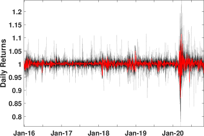
Table 5 summarizes the results, listing the variances of the daily returns. The S-q estimator performed the best with the lowest variance, which indicates high robustness. The MM-SHR performed the second best, followed by the S-Rocke. The sample estimator of mean and covariance was also included to demonstrate its poor robustness.
| Estimator | Variance |
|---|---|
| S-q | 76 |
| MM-SHR | 119 |
| S-Rocke | 147 |
| Sample | 176 |
Next, to demonstrate estimator efficiency, variances of daily returns were compared for a non-volatile period: 2016 through 2019. Using the same methodology and configuration as before, for each year and each estimator, and were estimated. Then, was calculated and applied to each day of that year. The sample variances of each year’s daily portfolio returns are listed in Table 6. The S-q estimator resulted in the lowest portfolio variance for three of the four years, and the lowest variance on average, indicating high estimator efficiency. On average, the performance of the MM-SHR estimator was behind that of the S-q estimator, and the S-Rocke demonstrated substantially worse performance.
| Year | S-q | MM-SHR | S-Rocke |
|---|---|---|---|
| 2016 | 3.51 | 3.56 | 4.10 |
| 2017 | 1.18 | 1.24 | 1.34 |
| 2018 | 6.76 | 6.91 | 7.31 |
| 2019 | 3.60 | 3.50 | 4.49 |
| Sample Mean | 3.77 | 3.80 | 4.31 |
8 Conclusion
The S-q estimator has been introduced as a new tunable multivariate estimator of location, scatter, and shape matrices for elliptical probability distributions. This new estimator is a subclass of S-estimators, which achieve the maximum theoretical breakdown point. The S-q estimator has been compared with the leading high-breakdown estimators. Across elliptical distributions, the S-q has generally higher efficiency and stability, and its robustness is on par with these other leading estimators. Additionally, the S-q provides a monotonic and upper-bounded efficiency tuning parameter, which provides simpler tuning than the MM-SHR. The S-q is therefore a broadly applicable estimator, providing practitioners with a good general high-breakdown multivariate estimator that can be used across a broad range of practical applications, such as the optimal portfolio example.
References
- Abusev (2015) Abusev, R.A., 2015. On the Distances Between Certain Distributions in Multivariate Statistical Analysis. Journal of Mathematical Sciences 205, 2–6. doi:10.1007/s10958-015-2222-y.
- Basu et al. (1998) Basu, A., Harris, I.R., Hjort, N.L., Jones., M.C., 1998. Robust and Efficient Estimation by Minimising a Density Power Divergence. Biometrika 85, 549–559.
- Bilodeau and Brenner (1999) Bilodeau, M., Brenner, D., 1999. Theory of Multivariate Statistics. Springer-Verlag, New York.
- Choi and Hall (2000) Choi, B.Y.E., Hall, P., 2000. Rendering Parametric Procedures More Robust by Empirically Tilting the Model. Biometrika 87, 453–465.
- Davies (1987) Davies, P.L., 1987. Asymptotic Behaviour of S-Estimates of Multivariate Location Parameters and Dispersion Matrices. The Annals of Statistics 15, 1269–1292.
- Deng and Yao (2018) Deng, X., Yao, J., 2018. On the property of multivariate generalized hyperbolic distribution and the Stein-type inequality. Communications in Statistics - Theory and Methods 47, 5346–5356. doi:10.1080/03610926.2017.1390134.
- Fang et al. (1990) Fang, K.T., Kotz, S., Ng, K.W., 1990. Symmetric Multivariate and Related Distributions. Chapman and Hall, London.
- Ferrari and Yang (2010) Ferrari, D., Yang, Y., 2010. Maximum Lq-likelihood estimation. The Annals of Statistics 38, 753–783. doi:10.1214/09-AOS687.
- Frahm (2009) Frahm, G., 2009. Asymptotic distributions of robust shape matrices and scales. Journal of Multivariate Analysis 100, 1329–1337. doi:10.1016/j.jmva.2008.11.007.
- Gazor and Zhang (2003) Gazor, S., Zhang, W., 2003. Speech probability distribution. IEEE Signal Processing Letters 10, 204–207. doi:10.1109/LSP.2003.813679.
- Huang et al. (2006) Huang, J.Z., Liu, N., Pourahmadi, M., Liu, L., 2006. Covariance matrix selection and estimation via penalised normal likelihood. Biometrika 93, 85–98. doi:10.1093/biomet/93.1.85.
- Huber (1964) Huber, P.J., 1964. Robust Estimation of a Location Parameter. The Annals of Mathematical Statistics 35, 73–101.
- Kelker (1970) Kelker, D., 1970. Distribution Theory of Spherical Distributions and a Location-Scale Parameter Generalization. Sankhyā: The Indian Journal of Statistics, Series A (1961-2002) 32, 419–430.
- Konlack Socgnia and Wilcox (2014) Konlack Socgnia, V., Wilcox, D., 2014. A comparison of generalized hyperbolic distribution models for equity returns. Journal of Applied Mathematics 2014. doi:10.1155/2014/263465.
- Lopuhaä (1989) Lopuhaä, H.P., 1989. On the Relation between S-Estimators and M-Estimators of Multivariate Location and Covariance. The Annals of Statistics 17, 1662–1683.
- Lopuhaä (1997) Lopuhaä, H.P., 1997. Asymptotic expansion of S-estimators of location and covariance. Statistica Neerlandica 51, 220–237. doi:10.1111/1467-9574.00051.
- Markowitz (1952) Markowitz, H., 1952. Portfolio Selection. The Journal of Finance 7, 77–91.
- Maronna (1976) Maronna, R.A., 1976. Robust M-Estimators of Multivariate Location and Scatter. The Annals of Statistics 4, 51–67.
- Maronna et al. (2006) Maronna, R.A., Martin, R.D., Yohai, V.J., 2006. Robust Statistics: Theory and Methods. First ed., John Wiley & Sons.
- Maronna et al. (2019) Maronna, R.A., Martin, R.D., Yohai, V.J., Salibián-Barrera, M., 2019. Robust Statistics Theory and Methods (with R). Second ed., John Wiley & Sons.
- Maronna and Yohai (2017) Maronna, R.A., Yohai, V.J., 2017. Robust and efficient estimation of multivariate scatter and location. Computational Statistics and Data Analysis 109, 64–75. doi:10.1016/j.csda.2016.11.006.
- Merton (1972) Merton, R.C., 1972. An Analytic Derivation of the Efficient Portfolio Frontier. The Journal of Financial and Quantitative Analysis 7, 1851–1872.
- Peña and Prieto (2007) Peña, D., Prieto, F.J., 2007. Combining Random and Specific Directions for Outlier Detection and Robust Estimation in High-Dimensional Multivariate Data. Journal of Computational and Graphical Statistics 16, 228–254.
- Rocke (1996) Rocke, D.M., 1996. Robustness Properties of S-Estimators of Multivariate Location and Shape in High Dimension. The Annals of Statistics 24, 1327–1345.
- Rousseeuw and Hubert (2013) Rousseeuw, P., Hubert, M., 2013. High-Breakdown Estimators of Multivariate Location and Scatter, in: Becker, C., Fried, R., Kuhnt, S. (Eds.), Robustness and Complex Data Structures. Springer, New York. chapter 4, pp. 49–66. doi:10.1007/978-3-642-35494-6.
- Rousseeuw and Yohai (1984) Rousseeuw, P., Yohai, V., 1984. Robust Regression by Means of S-Estimators, in: Robust and Nonlinear Time Series Analysis. Springer US : New York, NY. TA - TT -, pp. 256–272. doi:10.1007/978-1-4615-7821-5{\_}15.
- Roy (1952) Roy, A.D., 1952. Safety First and the Holding of Assets. Econometrica 20, 431–449.
- Tyler (1982) Tyler, D.E., 1982. Radial estimates and the test for sphericity. Biometrika 69, 429–436. doi:10.1093/biomet/69.2.429.
- Tyler (1983) Tyler, D.E., 1983. Robustness and effciency properties of scatter matrices. Biometrika 70, 411–420. doi:10.1093/biomet/71.3.656-a.
- Ward et al. (1990) Ward, K.D., Baker, C.J., Watts, S., 1990. Maritime surveillance radar. Part 1. Radar scattering from the ocean surface. IEE Proceedings F (Radar and Signal Processing) 137, 51–62. doi:10.1049/ip-f-2.1990.0009.
- Windham (1995) Windham, M.P., 1995. Robustifying Model Fitting. Journal of the Royal Statistical Society. Series B (Methodological) 57, 599–609.