New Homogeneous Dataset of Solar EUV synoptic maps from SOHO/EIT and SDO/AIA
Solar Physics
keywords:
SOHO, SDO; EUV, Synoptic Maps; Dataset1 Introduction
S-Introduction
Synoptic maps provide a convenient way to display the evolution/distribution of various physical quantities and features on the entire solar surface. For example, synoptic maps have been used to study coronal holes (CH) (Karna et al., 2015; Golubeva and Mordvinov, 2017; Hamada et al., 2018), photospheric and coronal magnetic fields (Virtanen and Mursula, 2016) and long-lived active regions (ARs). Solar synoptic maps can also be used to study the nonuniform structure of the EUV corona in both longitude and latitude, reflecting the nonuniform distribution of the large-scale magnetic field (Benevolenskaya, Kosovichev, and Scherrer, 2001). Different ground-based observations of the photospheric magnetic field are also presented in the form of synoptic maps (e.g., Wilcox Solar Observatory, National Solar Observatory, Mount Wilson Observatory and Kitt Peak Vacuum Telescope).
Synoptic maps are constructed by concatenating a series of meridian strips taken from full-disk images covering a full Carrington Rotation (CR) of 27.2753 consecutive days. Each individual full-disk image is remapped into heliographic coordinates with longitude along the x-axis, and latitude (or sine-latitude) along the y-axis. A rigid solar rotation rate is often assumed in order to reduce the effects of the dynamic surface of the Sun to the synoptic maps (Harvey and Worden, 1998).
In this study, we present a new dataset of EUV synoptic maps, based on Extreme Ultraviolet Imaging Telescope (EIT) and Atmospheric Imaging Assembly (AIA) observations on board of Solar and Heliospheric Observatory (SOHO) and Solar Dynamics Observatory (SDO), respectively. These maps are constructed homogeneously with the same methodology and daily resolution (13.3∘ wide central solar meridian strip) for both instruments and finally inter-calibrated to eliminate the differences in intensity distribution between the two instruments. Moreover, SDO/AIA data are used to construct also EUV synoptic maps with much more narrow meridian strips (1.1∘ wide) representing a closer match between time and longitude in synoptic maps.
This paper is organized as follows. Section \irefS-Previous_dataset presents techniques previously used to construct EUV synoptic maps from SOHO/EIT and SDO/AIA images. Section \irefS-data_analysis discusses EIT and AIA full-disk images, presenting the filtration and calibration criteria used to avoid corrupted images and to correct certain other problems. Section \irefS-synop_maps discusses the procedure for constructing the synoptic maps, including projection to heliographic coordinates, stripping, and merging of strips into a continuous synoptic map. The new dataset is compared with other publicly available datasets, and improvements are discussed. Section \irefS-eit_aia discusses the homogenization of EIT maps with AIA maps, providing a continuous and uniform dataset. Section \irefS-Summary summarizes our results.
2 Previous EUV synoptic map datasets
S-Previous_dataset
SOHO/EIT instrument (Delaboudinière et al., 1995) takes images of the Sun in four passbands that are centered on intense emission lines of the solar EUV spectrum. He II (304Å), Fe XI/Fe X (171Å), Fe XII (195Å), and Fe XV (284Å) lines provide temperature diagnostics in the range from 6 to 3 . These different wavelengths represent solar layers at different altitudes. He II 304Å images are dominated by emissions from structures of the transition region network (Benevolenskaya, Kosovichev, and Scherrer, 2001), indicating the magnetic footpoints of coronal loops and outlining the bases of coronal holes. Fe XI/Fe X 171Å images display background emission that is present over most of the quiet Sun (QS), while the most intense emission comes from active regions with closed magnetic field. Fe XII 195Å images are also dominated by emission from the closed magnetic field regions of the Sun, showing the inner solar corona with different distributions of intensities for CHs and the QS. The Fe XV 284Å passband allows an analysis of the hotter active regions.
For SDO/AIA instrument (Lemen et al., 2012), solar images are taken at 7 wavelengths in EUV (304Å, 171Å, 193Å, 211Å, 335Å, 94Å, 131Å) and 3 in UV/visible (white light, 1700Å, 1600Å). Only four EUV channels (304Å, 171Å, 193Å and 211Å) are selected here in order to be compatible with EIT. Table \irefT1 summarizes the characteristics of selected EIT and AIA wavelengths (Moses et al., 1997; Petkaki et al., 2012). Although there are subtle differences in the temperature response functions of the AIA/193Å and EIT/195Å channels, they are similar enough to be used together to generate synchronic maps (Caplan, Downs, and Linker, 2016). The EUV emissions of AIA/211Å and EIT/284Å originate from different ions in the corona, Fe-XIV and Fe-XV, respectively. However, the temperature responses of these two spectral lines have a large overlap and both peak close to each other at about 2.0 MK temperature (Moses et al., 1997; Petkaki et al., 2012). Therefore it is unlikely that there are large systematic differences between the AIA/211Å and EIT/284Å images.
| Source | Wavelength | Ion | Peak Temperature (MK) |
|---|---|---|---|
| SOHO/EIT | 284Å | Fe XV | 2.0 |
| SDO/AIA | 211Å | Fe XIV | 2.0 |
| SOHO/EIT | 195Å | Fe XII | 1.6 |
| SDO/AIA | 193Å | Fe XII | 1.6 |
| SOHO/EIT and SDO/AIA | 171Å | Fe IX-X | 1.3 |
| SOHO/EIT and SDO/AIA | 304Å | He II | 0.08 |
Currently, there are two incomplete EUV synoptic map datasets based on SOHO/EIT observations and one synoptic map dataset based on SDO/AIA observations. Benevolenskaya, Kosovichev, and Scherrer (2001) constructed SOHO/EIT synoptic maps in three Fe (171Å, 195Å, 284Å) lines and He II (304Å) from CR 1911 (1996 June 28) to CR 2055 (2007 March 31) by concatenating 16∘ wide central meridian strips. The size of these synoptic maps is 167 360 pixels with a resolution of of heliographic latitude and longitude covering all longitudes (1∘ to 360∘) and most latitudes ( to , leaving out those polar latitudes that are not always visible). These EIT synoptic maps are provided by Stanford Solar Observatories Group (SSOG) (http://sun.stanford.edu/synop/EIT/index.html). Although for every synoptic map, both sine and linear latitude GIF images were presented, the files offered in FITS (Flexible Image Transport System) format are in linear latitude only. Also, the maps from CR 1911 (1996 June 28) to CR 2042 (2006 April 10) are based on calibrated data, and from CR 2043 (2006 May 08) to CR 2055 (2007 March 31) on preliminary calibrated data.
Another set of EIT synoptic maps for only three wavelengths (171Å, 195Å and 304Å) are provided by the Space Weather Lab (SWL) at George Mason University (http://spaceweather.gmu.edu/projects/synop/EITSM.html) (Hess Webber
et al., 2014). The available maps extend from CR 2058 (2007 June 21) to CR 2102 (2010 October 03). Thus, the SSOG maps and the SWL maps are disparate and have a gap of two Carrington rotations in-between. In the SWL maps, central meridian longitudinal strips of 13.63∘ width have been concatenated using four images per day with 3/4 overlap between adjacent strips. The size of these synoptic maps is 36001080 pixels () and cover all longitudes and all measured latitudes at best up to . There are many missing maps in this dataset (23 out of 45 CRs) but the corresponding FITS files exist in both sine and linear latitude.
The only dataset of SDO/AIA synoptic maps is provided by SWL (http://spaceweather.gmu.edu/projects/synop/AIASM.html) from CR 2097 (2010 May 20) to CR 2186 (2017 January 10) (Karna, Hess Webber, and
Pesnell, 2014). The resolution and latitudinal extent is the same as that of SWL/EIT synoptic maps (13.63∘ wide central meridian strips). Also, the maps are provided only for three wavelengths (171Å, 193Å and 304Å). The maps from CR 2097 (2010 May 20) to CR 2124 (2012 May 25) are available in sine and linear latitude while from CR 2125 (2012 June 21) to CR 2186 (2017 January 10) the maps are available in linear latitude only. The temporal coverage of all the three databases of SOHO/EIT and SDO/AIA synoptic maps are summarized in Table \irefT2. Figure \irefF1 shows a sample of synoptic maps for the four EUV wavelengths from the three datasets. Many of the maps contain a data gap (represented as a white space in SSOG/EIT maps in Fig. \irefF1, first column). Also, sharp edges between adjacent longitudinal strips are observed in most of the maps from all datasets (Fig. \irefF1, second column). Maps of some wavelengths are missing for some specific Carrington rotations. For example, EIT/195Å map is missing for CR 2103 in SWL/EIT maps (Figure \irefF1, second row; second column). For SWL/AIA maps, it also seems that the camera’s exposure time and the image quality key-factors are not taken into account in the map preparation which is sometimes seen as overexposed (or underexposed) strips in the synoptic maps (for an example see Figure \irefF1, 3rd column, bottom row).
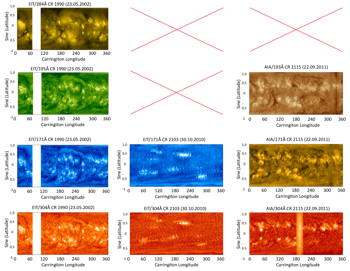
While inspecting these synoptic maps, we (Hamada et al., 2018) have earlier noted on the degradation of the AIA instrument with time and on differences in pixel intensity histograms due to different sensor responses of EIT and AIA. We also found that the SWL maps erroneously contained the RGB values of pixels instead of line intensity. This error has been corrected in the SWL dataset since then (N. Karna, 2017, private communication). In a subsequent, more detailed inspection, we have found, as noted above, that sharp edges often appear between adjacent strips in most EIT and AIA synoptic maps.
| Source | Observable | Start | End | ||
|---|---|---|---|---|---|
| CR | Date | CR | Date | ||
| SSOG | SOHO/EIT: 284Å, 195Å, 171Å, 304Å | 1911 | 1996.06.28 | 2055 | 2007.03.31 |
| SWL | SOHO/EIT: 195Å, 171Å, 304Å | 2058 | 2007.06.21 | 2102 | 2010.10.03 |
| SWL | SDO/AIA: 193Å, 171Å, 304Å | 2097 | 2010.05.20 | 2186 | 2017.01.10 |
In this paper, we use SOHO/EIT and SDO/AIA full-disk images to construct a new dataset of synoptic maps using strips of same width (13.3∘) for both EIT and AIA. Additionally we construct AIA maps also with narrower 1.1∘ strips which allow better correspondence of synoptic map longitudes with the central solar meridian.
3 Data analysis
S-data_analysis
Full-disk solar images from both SOHO/EIT and SDO/AIA are used to construct the new EUV synoptic maps. SOHO/EIT images are available from January 1996 until the end of December 2018 while SDO/AIA images are available from May 2010 until present.
Table \irefT3 shows SOHO/EIT and SDO/AIA full-disk data intervals used in this study. Each full-disk image was
automatically checked to avoid any corrupted/noisy data.
| Source | Observable | Start | End |
|---|---|---|---|
| SOHO/EIT | 284Å, 195Å, 171Å and 304Å | 1996.01.16 | 2018.12.31 |
| SDO/AIA | 211Å, 193Å, 171Å and 304Å | 2010.05.13 | 2018.12.31 |
3.1 SOHO/EIT
S-soho_eit
SOHO/EIT full-disk images were downloaded from the SOHO Science Archive (SSA) hosted at the European Space Astronomy Centre (ESAC), and National Aeronautics and Space Administration (NASA). SOHO has an extensive database including over 20 years of data from 1996 to 2018 (Table \irefT3). EIT routinely takes one image in each of its four wavelengths several times per day. Each image is 1024 1024 pixels, corresponding to a resolution of 2.6 arcsec per pixel.
We used different keywords to identify different types of image deficiencies and noise.
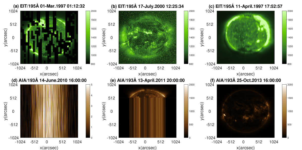
Keyword N_MISSING_BLOCKS represents the number of missing blocks in the EIT images due to, e.g., unstable EIT telemetry (for an example see Figure \irefF2a). Another reason for poor image quality are solar energetic particles, which can greatly increase the image noise (for an example see Figure \irefF2b). We used the mean intensity of the off-limb area as a measure to eliminate the noisy images. In addition to missing blocks and noise the EIT images may be subject to a higher level of scattered light (Scherrer et al., 2012). All images with enhanced noise or corrupted/missing pixel blocks are discarded and only good quality images were processed. Keyword EXPTIME was used to avoid all images with very high or low exposure times (Figure \irefF2c). SC_ROLL keyword represents the roll angle offsets from the projection of the Sun’s North Pole and it is used to ensure that the solar north is at top of the image.
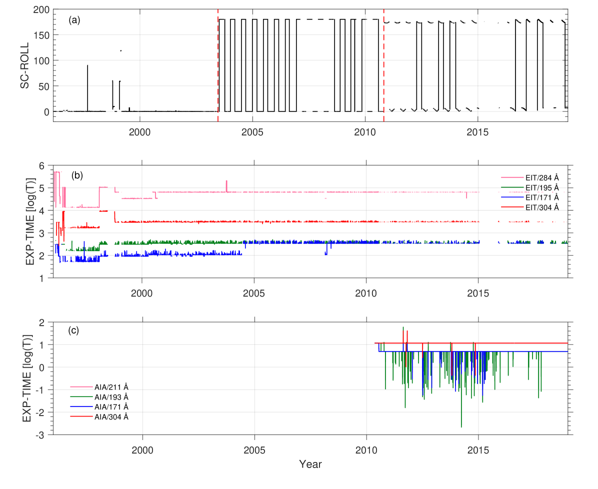
Since June 19, 2003, due to a malfunction in the antenna pointing mechanism, SOHO’s signals were relayed primarily on the backup antenna. Because of this the spacecraft is systematically rolled by 180∘ around the solar direction every three months in order to have the Earth constantly in the antenna’s field of view as the spacecraft and the Earth progress in their respective orbits (Figure \irefF3a). After October 29, 2010, the spacecraft is no longer aligned with the solar rotation axis but to the Ecliptic North Pole. Therefore, the roll angle with respect to the solar rotation axis goes from -7.25∘ in June to 7.25∘ in December. Figure \irefF3b,c shows the variation of the logarithmic EIT and AIA exposure times (EXPTIME) at different spectral lines.
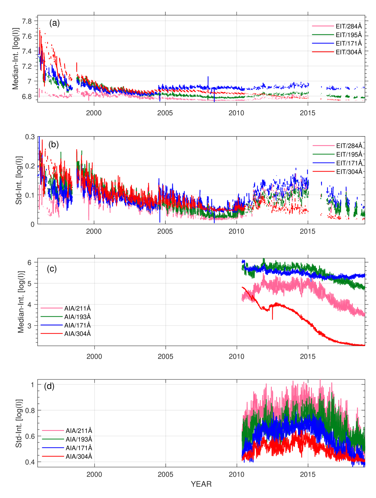
Figures \irefF4a-b show the median and standard deviation of logarithmic pixel intensities of SOHO/EIT full-disk images for wavelengths 284Å, 195Å, 171Å and 304Å. Only the median intensity of 284Å shows a somewhat steady variation throughout the entire depicted time interval. On the other hand, median intensities of 195Å, 171Å and 304Å decrease especially during the first five years (1996-2001). This decrease is likely caused by the degradation of EIT sensitivity. The most significant degradation is observed in 304Å intensity which had the highest values in 1996 and decreased systematically until 2004, increased a bit in 2005 and declined thereafter until 2016. The standard deviations of the intensities of different wavelengths show a slightly more systematic temporal evolution than the median
intensities with lowest values around the solar minimum in 2008-2009, and a fairly clear variation over the solar cycle 23/24.
3.2 SDO/AIA
S-sdo_aia
SDO/AIA images were downloaded from Joint SDO Operations Centre (JSOC), located at Stanford University. The FITS images at JSOC are based on level 1.5 data with a 2-minute cadence reduced to 2.4 arcsec pixels corresponding to 10241024 pixel resolution. These images are produced approximately 7 days after the time of observation from level 1 definitive data. The keywords QUALITY and EXP_TIME are used to check for image corruption (for examples see Figures \irefF2d-e) and to identify significantly overexposed or underexposed images (see, e.g., Figure \irefF2f), respectively. Note that the QUALITY keyword also indicates the enhanced noise caused by solar particles.
Median and standard deviation of SDO/AIA logarithmic intensities are shown in Figure \irefF4c-d. Again, a fairly systematic evolution over the solar cycle 24 is seen in the standard deviations (Figures \irefF4d) and partly also in the median intensities of 211Å and 193Å wavelengths (Figure \irefF4c) which correspond to the outer layers of the corona. The 304Å intensity shows significant degradation, although intensity increased momentarily in September 2011 due to instrument bake-outs (Boerner et al., 2014). Degradation has been suggested to result from the accumulation of volatile contamination on the optics or detector telescopes (Boerner et al., 2014). Due to the differences in the instrument calibrations, degradation and operating orbit, the spectral line intensities of SOHO/EIT and SDO/AIA show a quite different temporal evolve over the overlapping time interval.
4 EUV Synoptic maps
S-synop_maps
For each EUV full-disk image, we extract the information included within the image FITS header. This information includes the radius of the Sun in pixels (R_SUN), Carrington longitude/latitude of the center of the solar disk (CRLN_OBS/CRLT_OBS) and Carrington rotation number (CAR_ROT). The value of the solar photospheric radius (R_SUN) is used to remove the off-limb measurements and to fix the image boundaries to the solar limb (see Figures \irefF5a-b). Carrington latitude (CRLT_OBS) of the disk center, the so-called angle, changes annually due to the tilt of the solar equator by with respect to the Earth’s ecliptic plane. This tilt also gives the Earth (or SOHO and SDO) a better view of the northern (southern) solar pole during fall (spring). The angle also affects the observed intensities in the following way: during fall (spring) the length of the line-of-sight path through the coronal matter to the southern (northern) hemisphere increases, which increases (decreases) the observed intensity of the EUV emission (Hamada et al., 2018).
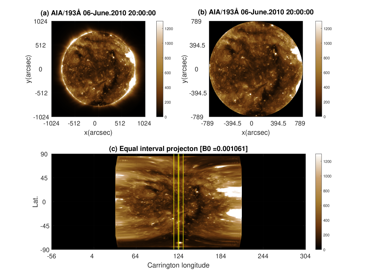
After removing the off-limb pixels from full-disk images the visible solar disk is projected from image plane coordinates (X,Y) into heliographic latitude/longitude coordinates on the spherical solar surface (,). In this projection the full-disk images are mapped to equal interval latitude-longitude grids (-90∘ to +90∘ latitude and longitude around the central meridian Carrington longitude) having 14403600 pixels. The cartesian heliographic coordinates of an image plane point with pixel coordinates and (these being zero at the center of the solar disk in the full-disk image) are
| (1) | |||||
| (2) | |||||
| (3) |
where is the solar radius in pixels and
| (4) | |||||
| (5) |
The heliographic latitude () and longitude () are then obtained from
| (6) | |||||
| \ilabeleq˙phi | (7) |
where is the Carrington longitude of the central solar meridian (CRLT_OBS).
The synoptic maps are constructed by concatenating meridional strips around the central solar meridian
taken from the projected full-disk images. The image cadence of SOHO/EIT is typically several hours and
often the SOHO/EIT dataset contains gaps of several days. Because of this we selected 13.3∘ wide strips for
SOHO/EIT, which corresponds to 1 image/day (dashed vertical lines in Figure \irefF5c). For SDO/AIA the image cadence is higher. Thus, for SDO/AIA we produced two sets of synoptic maps, one using a central solar meridian strips 1.1∘ wide and another using 13.3∘ wide strips. The SDO/AIA maps with 13.3∘ strip width are thus constructed to be compatible with the SOHO/EIT maps that have the same strip width.
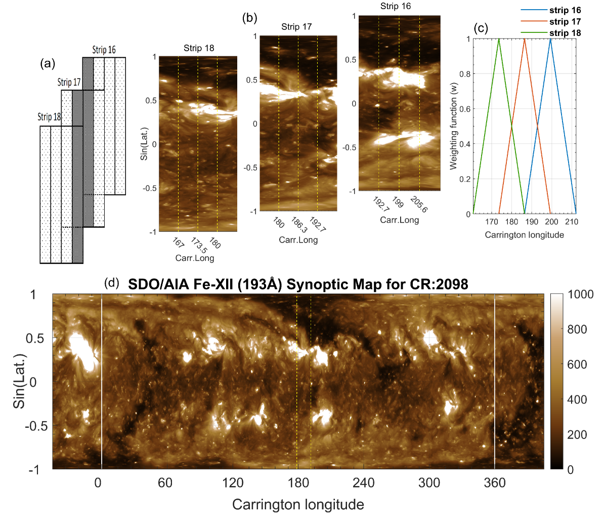
Figure \irefF6 shows how the synoptic maps are constructed by including all the projected full-disk images belonging to the corresponding Carrington rotation, taking from each the central meridian strip and overlapping the neighbouring strips by half of their width. As an example see the central strip (no.17) in Figure \irefF6 which is half overlapped with the previous and next strips 16 and 18 (Figure \irefF6a), respectively. The overlapped parts (see Figure \irefF6b), are averaged using a linearly varying weighting function (Figure \irefF6c) that drops from one at strip center to zero at the strip edge. The pixel intensity at Carrington longitude can be expressed as
| (8) |
where loops through all the central meridian strips taken from the projected full-disk images, including the corresponding longitude of of the same Carrington rotation. The weighting functions of each strip are defined as
| (9) | |||||
| (10) |
where is the central Carrington longitude of the :th strip (see also Eq. \irefeq_phi) and
is the width of the strip in degrees.
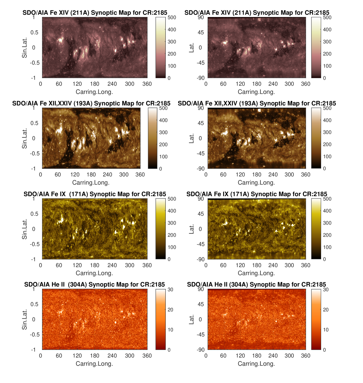
Sometimes there are relatively long gaps in the AIA or EIT datasets, which would result in gaps in the synoptic maps if the strip width remained constant. To fill in such gaps we extend the strips equally on both sides of the data gap up to a maximum of 3 days (i.e., about 40.89∘). The strip width is limited because extending the strips too much would start introducing significant distortions due to projection effects (see Figure \irefF5c). All the final synoptic maps have a resolution of 14403600 pixels, covering all measured latitudes from -90∘ to +90∘ and longitudes from 0∘ to 360∘. Note however, that because of visibility limitation related to the annual -angle variation there is an annually varying data gap at polar latitudes. For each Carrington rotation, the maps are produced both in linear and sine latitude. Figure \irefF7 shows an example of the constructed synoptic maps of CR 2185 in sine and linear latitude for SDO/AIA 211Å, 193Å, 171Å, and 304Å. For SDO/AIA, EUV synoptic maps were constructed from Carrington rotation CR 2097 (2010 May 20) to CR 2204 (2018 May 16) while for SOHO/EIT the maps were constructed from CR 1906 (1996 Feb 19) to CR 2212 (2018 Dec 20) (Table \irefT4).
| Observable | Start | End | ||
|---|---|---|---|---|
| CR | Date | CR | Date | |
| SOHO/EIT: 284Å, 195Å, 171Å and 304Å | 1906 | 1996.02.13 | 2212 | 2018.12.20 |
| SDO/AIA: 211Å, 193Å, 171Å and 304Å | 2097 | 2010.05.20 | 2212 | 2018.12.20 |
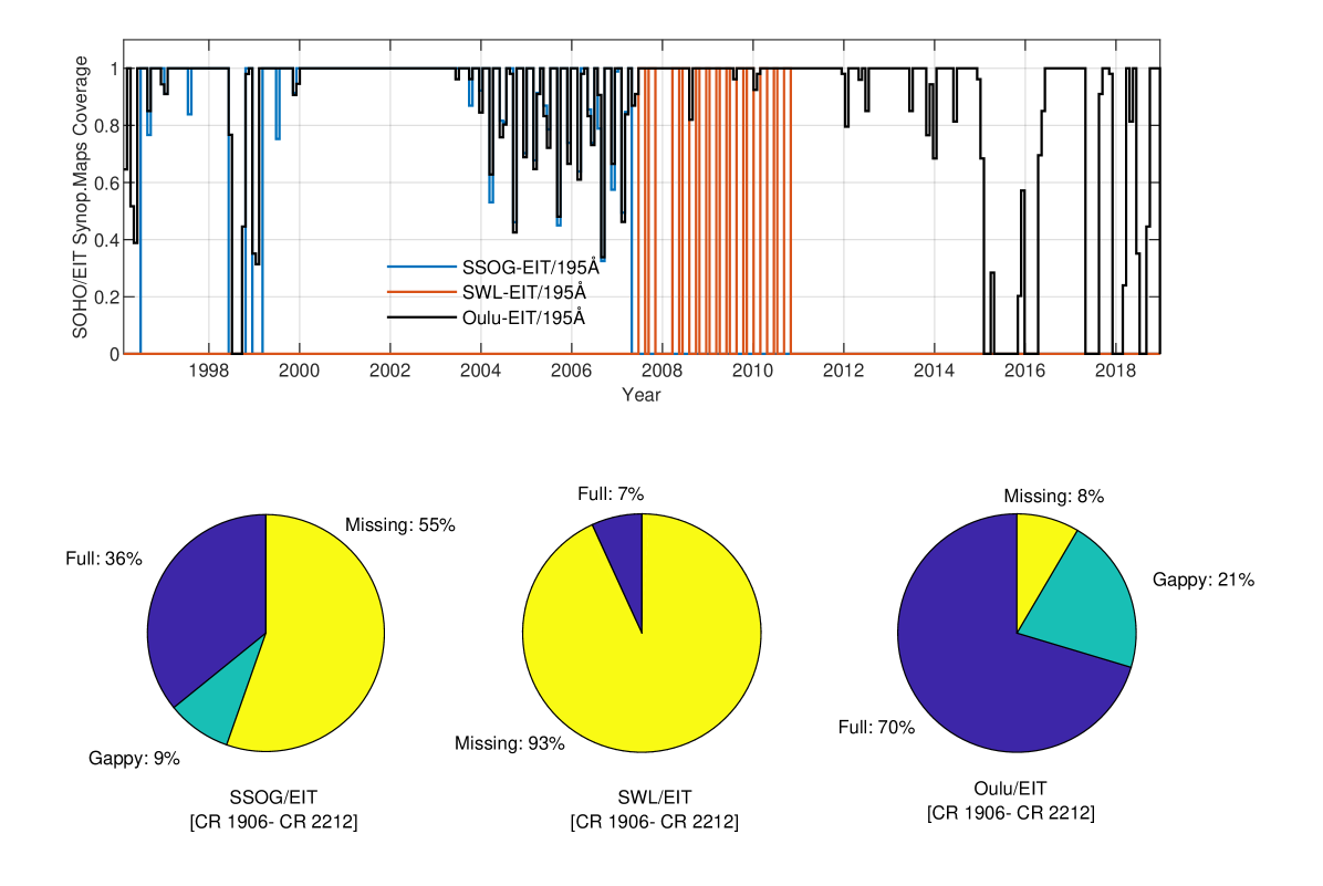
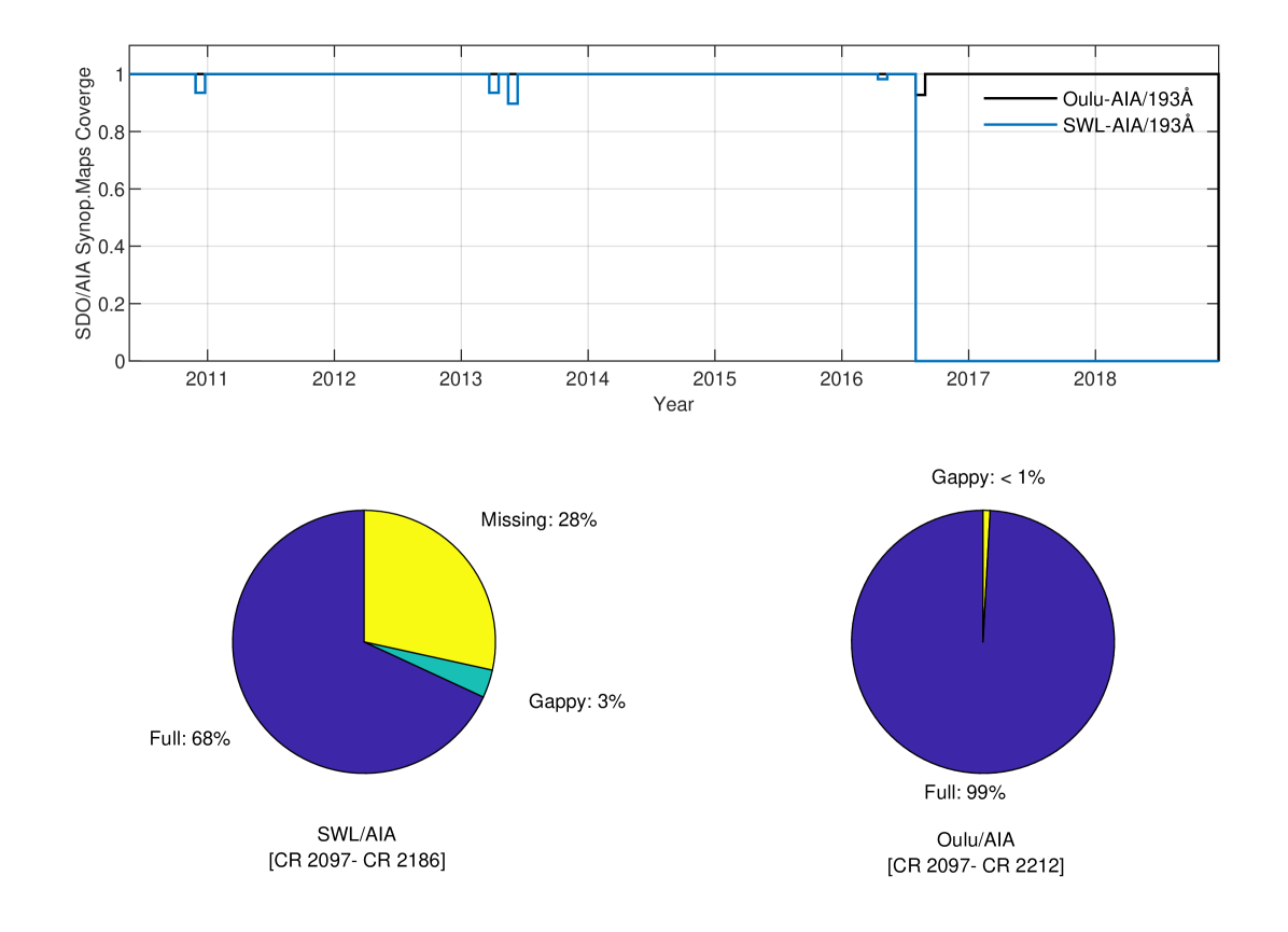
In comparison to the existing SOHO/EIT and SDO/AIA synoptic map datasets from SSOG and SWL, the new maps constructed here provide a longer and homogeneous dataset with fewer data gaps. To demonstrate this, Figures \irefF8 and \irefF9 show EIT/195Å and AIA/193Å data coverages as a pie chart representing the overall fraction of full, gappy and missing synoptic maps, respectively. Overall the SOHO/EIT full-disk image dataset available from February 1996 until December 2018 covers 307 Carrington rotations. SWL provides only 21 full synoptic maps for SOHO/EIT, and SSOG 110 full maps. In contrast, our new dataset contains a total of 216 full maps for this period and, thus, considerably extends the coverage compared to the SSOG and SWL datasets. This number of full maps includes those gappy ones filled up to 3 missing days.
For SDO/AIA, the full-disk images are available from CR 2097 (May 2010) until present. The SDO/AIA synoptic maps offered by SWL extend until CR 2186 with a total of 79 full maps (68%) and 4 gappy maps (3%), respectively, while our new dataset is almost complete until CR 2215, with 118 (99%) of Carrington rotations are fully covered and only one map (less than 1%) containing gappy synoptic maps.
5 Homogenization of SOHO/EIT and SDO/AIA synoptic maps
S-eit_aia
Because of instrumental differences the overall intensity distributions of SOHO/EIT and SDO/AIA images of corresponding wavelengths are very different. As an example of this, Figure \irefF10 shows AIA 193Å (Fig. \irefF10a) and EIT 195Å (Fig. \irefF10c) synoptic maps for CR 2114 in logarithmic intensity scale. Panels b and d in Figure \irefF10 display the histogram and cumulative histogram of their logarithmic intensities. One can see a dramatic difference between AIA and EIT in the form of the intensity distributions (Fig. \irefF10b) and the range of intensities they cover. It is clear that in order to have a homogeneous composite dataset combining the two instruments, the synoptic maps from the two instruments need to be inter-calibrated to the same level. Here we choose to transform the EIT maps to AIA level.
Before inter-calibration all the EIT and AIA synoptic map data are converted to logarithmic scale and then standardized separately for each map by subtracting the average logarithmic intensity of the map and dividing by the standard deviation of logarithmic intensity of the corresponding map. We used logarithmic intensities because in linear scale the intensity distributions are extremely skewed. In logarithmic scale the histograms are much more Gaussian and the distribution mean and standard deviation better represent the center and spread of values. The smoother and more symmetric histograms also allow a more accurate determination of cumulative probabilities for each pixel value, which is important for the homogenization as will be discussed below. Standardization scales the synoptic map histograms to the same level and thereby, e.g., removes the intensity changes related to instrument degradation. However, these changes are very difficult to separate from real, e.g., solar cycle related changes. Standardized synoptic maps describe relative intensity variations within each map, and thus do not have this problem. Note that, these synoptic maps cannot be used to study the long-term changes of the average EUV intensities, only the relative intensity variations and relative spatial distribution changes. Figures \irefF10e and \irefF10g show the standardized SDO/AIA and SOHO/EIT synoptic maps for CR 2114, while \irefF10f and \irefF10h show the corresponding histograms and cumulative histograms. One can see that the standardization of logarithmic intensities improves the agreement between the EIT and AIA maps and corresponding histograms. However, significant differences still remain, which is seen in the different form of the two histograms. The EIT–AIA inter-calibration aims to eliminate these differences in the form of the histograms by finding a transformation that brings the SOHO/EIT histogram as close to the corresponding SDO/AIA histogram as possible.
The inter-calibration is based on comparing 93 simultaneous full synoptic maps from EIT and AIA between CR 2097- CR 2212. For all these maps we first compute the histogram of standardized logarithmic intensity and then compute the overall average histograms for those 93 CRs, separately for SOHO/EIT and SDO/AIA. We then form the corresponding overall cumulative histograms. Using these two cumulative histograms we compute for each value of SOHO/EIT standardized log-intensity the corresponding SDO/AIA standardized log-intensity , which has the same cumulative probability value in its respective histogram as the SOHO/EIT value. The difference of these values, i.e., is a function of the SOHO/EIT standardized log-intensity and indicates by how much the standardized log-intensities of SOHO/EIT pixels should be changed in order for the pixel value to correspond to the AIA level. Thus, the scaled standardized log-intensities of SOHO/EIT pixels are obtained by equation
| (11) |
This scaling inter-calibration procedure is performed for each synoptic map of the four wavelengths separately. The same procedure is applied to all EIT maps including those ones that were not used to determine the EIT/AIA inter-calibration. The relationships between the scaled and original standardized log-intensities for the four EIT wavelengths are shown in Figure \irefF11. The figure also indicates the one-to-one line as a reference. One can see that for all four wavelengths the intensities between -3 and 0 (i.e., up to 3 standard deviations below the mean) are decreased from the original value by scaling. Intensities between about 0 and 3 are (i.e., up to 3 standard deviations above the mean intensity) are increased by the scaling. Finally the very dark values (-4) are increased and the very bright values (4) are decreased by scaling.
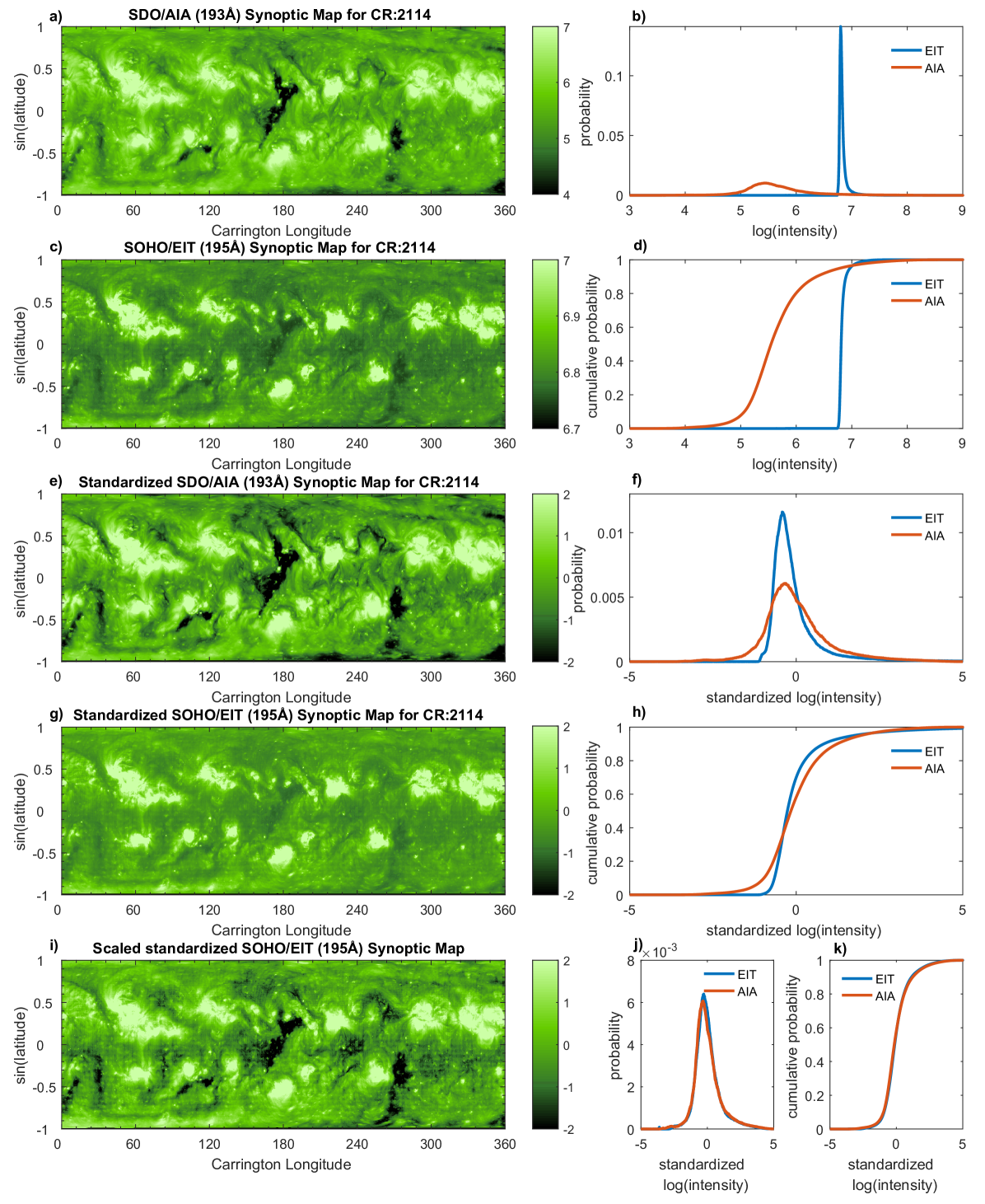
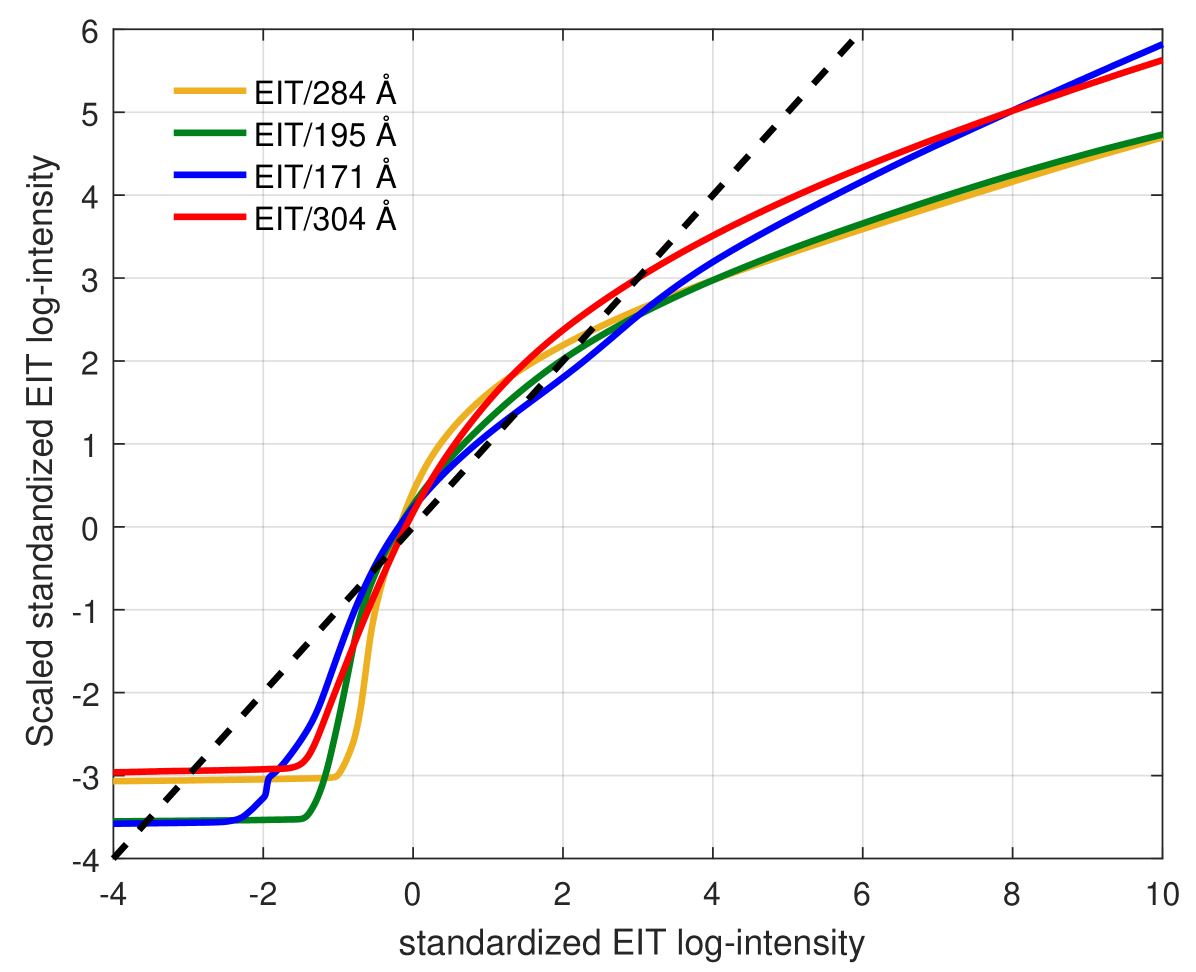
Figure \irefF10i shows the scaled standardized SOHO/EIT synoptic map, which should be compared with the standardized SDO/AIA synoptic map shown in Figure \irefF10e. Visual comparison between these two synoptic maps shows that they are very similar. The contrast and range of standardized intensity values are roughly the same and, e.g., dark coronal holes seem to be resolved quite similarly in both maps. Figures \irefF10j and \irefF10k show the histograms and cumulative histograms, respectively, of the scaled standardized SOHO/EIT map and standardized SDO/AIA map. One can see that the scaling (inter-calibration) procedure discussed above efficiently transforms the EIT histogram to closely match with the corresponding AIA histogram, thereby validating the inter-calibration for CR 2114. The same is true also for all the other maps used in the inter-calibration.
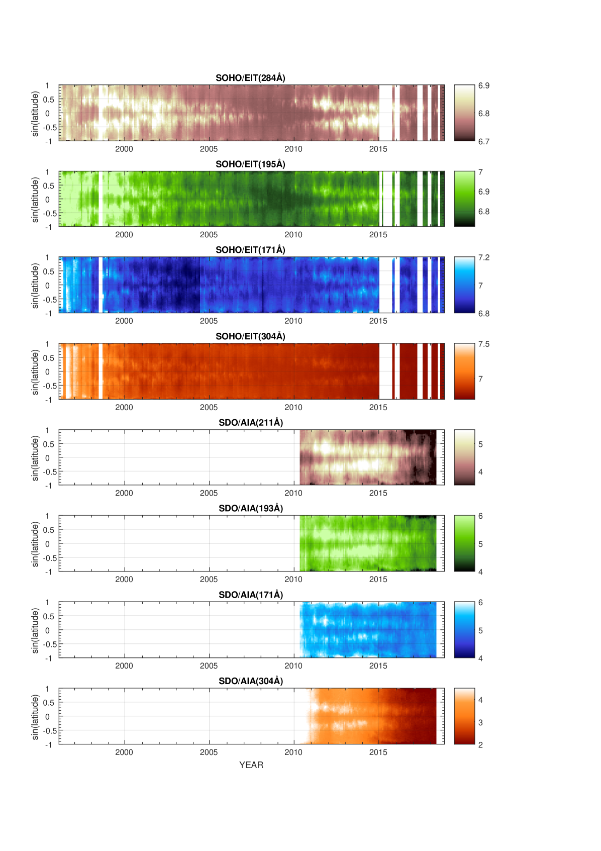
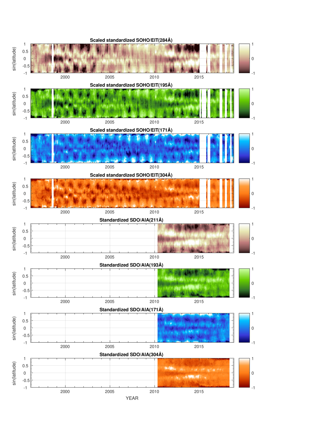
Figure \irefF12 shows a broad overview of logarithmic EUV intensities of the SOHO/EIT (first four rows) and SDO/AIA (bottom four rows) synoptic maps over the entire time interval covered by the maps. The intensity distributions in Fig. \irefF12 are obtained from the synoptic maps by averaging over Carrington longitude. One can see the previously discussed drifts in the SOHO/EIT intensities in all the four wavelengths (see Figure \irefF4a,b and related discussion).
For SDO/AIA such a drift is especially visible in the 304Å wavelength. In addition, the 171Å wavelength of SOHO/EIT displays an abrupt change in the intensity distribution in 2004, which was also seen in Figure \irefF4c,d.
As a comparison to Figure \irefF12, Figure \irefF13 shows the corresponding relative EUV intensities obtained from the final homogenized SOHO/EIT and SDO/AIA synoptic maps, i.e., with scaled standardized log-intensities for EIT and standardized log-intensities for AIA. Here one can see that standardization effectively removes the above discussed temporal drifts in the overall intensity, from both datasets. It should be noted that standardization also removes the real solar cycle related variation of intensities. However, for the main purpose of producing these relative intensity maps, i.e., the determination of coronal holes, this is not a problem. The scaling of SOHO/EIT maps brings them to the same relative intensity level as the corresponding AIA maps. Visual inspection of the corresponding wavelengths in Fig. \irefF13 shows that the two datasets produce indeed very similar distributions for the corresponding wavelengths.
6 Summary
S-Summary
In this study we presented a new dataset of EUV synoptic maps based on SOHO/EIT and SDO/AIA full disk images. The new dataset differs from the previously existing datasets in several ways. First of all, the new synoptic maps have been constructed using the same spatial resolution (13.3∘ wide central solar meridian strip) for both instruments thereby reducing the differences between the maps that may result from different image resolution or different image sampling frequency. We have also used the entire set of full-disk images available at the time of writing and thereby notably extended the coverage of synoptic maps compared to the previous datasets. Taking advantage of the higher image cadence in SDO/AIA we also constructed another set of SDO/AIA synoptic maps with narrower central meridian strips (1.1∘ wide) which allow each synoptic map longitude to better correspond to the central solar meridian. Secondly, in order to avoid the problems due to significant and complicated drifts in the SOHO/EIT and SDO/AIA intensities, we standardized the synoptic maps in logarithmic intensity scale. While this procedure inevitably removes the real, e.g., solar cycle related intensity variations it produces a more homogeneous dataset of relative intensities for the purpose of studying the evolution of coronal structures, e.g., coronal holes. Thirdly, even after standardizing the synoptic maps the relative intensity distributions of the corresponding SOHO/EIT and SDO/AIA synoptic maps are very different due to instrumental differences. In order to remove these differences between the EIT and AIA maps we developed a method to scale the EIT pixel values to the AIA level. The scaling is based on comparing the overall average cumulative histograms of 93 simultaneous EIT and AIA synoptic maps and determining how much the EIT standardized log-intensities should be changed so that their overall cumulative probability matches that of AIA. As a result of this scaling the simultaneous EIT and AIA synoptic maps are very close to each other. Overall, this work resulted in a new homogenized and standardized database of solar EUV synoptic maps from SOHO/EIT and SDO/AIA. The constructed maps describe relative logarithmic intensity variations within each map. These maps are well suited for studying the evolution of different coronal structures such as coronal holes over solar cycle timescales, where data homogeneity is important.
Acknowledgments
The dataset constructed here is available by request to the authors (A. Hamada, amr.hamada@oulu.fi; T. Asikainen, timo.asikainen@oulu.fi or K. Mursula, kalevi.mursula@oulu.fi). We acknowledge the financial support by the Academy of Finland to the ReSoLVE Center of Excellence (project No. 307411).
References
- Benevolenskaya, Kosovichev, and Scherrer (2001) Benevolenskaya, E.E., Kosovichev, A.G., Scherrer, P.H.: 2001, Detection of high-latitude waves of solar coronal activity in extreme-ultraviolet data from the Solar and Heliospheric Observatory EUV Imaging Telescope. Astrophys. J. 554, L107. DOI. http://iopscience.iop.org/1538-4357/554/1/L107.
- Boerner et al. (2014) Boerner, P.F., Testa, P., Warren, H., Weber, M.A., Schrijver, C.J.: 2014, Photometric and thermal cross-calibration of solar euv instruments. Solar Phys. 289(6), 2377. DOI. https://doi.org/10.1007/s11207-013-0452-z.
- Caplan, Downs, and Linker (2016) Caplan, R.M., Downs, C., Linker, J.a.: 2016, Synchronic Coronal Hole Mapping Using Multi-Instrument Euv Images: Data Preparation and Detection Method. Astrophys. J. 823(1), 53. DOI. http://stacks.iop.org/0004-637X/823/i=1/a=53?key=crossref.5a3dd7d05530bc097ecc3a0dc7ece526.
- Delaboudinière et al. (1995) Delaboudinière, J.-P., Artzner, G.E., Brunaud, J., Gabriel, A.H., Hochedez, J.F., Millier, F., Song, X.Y., Au, B., Dere, K.P., Howard, R.A., Kreplin, R., Michels, D.J., Moses, J.D., Defise, J.M., Jamar, C., Rochus, P., Chauvineau, J.P., Marioge, J.P., Catura, R.C., Lemen, J.R., Shing, L., Stern, R.A., Gurman, J.B., Neupert, W.M., Maucherat, A., Clette, F., Cugnon, P., Van Dessel, E.L.: 1995, EIT: Extreme-UltraViolet Imaging Telescope for the SOHO Mission. In: The SOHO Mission, Springer, Dordrecht, 291. DOI. http://link.springer.com/10.1007/978-94-009-0191-9_8.
- Golubeva and Mordvinov (2017) Golubeva, E.M., Mordvinov, A.V.: 2017, Rearrangements of open magnetic flux and formation of polar coronal holes in cycle 24. Solar Phys. 292(11), 175. DOI. https://doi.org/10.1007/s11207-017-1200-6.
- Hamada et al. (2018) Hamada, A., Asikainen, T., Virtanen, I., Mursula, K.: 2018, Automated identification of coronal holes from synoptic euv maps. Solar Phys. 293(4), 71. DOI. https://doi.org/10.1007/s11207-018-1289-2.
- Harvey and Worden (1998) Harvey, J., Worden, J.: 1998, New Types and Uses of Synoptic Maps. In: Balasubramaniam, K.S., Harvey, J., Rabin, D. (eds.) Synoptic Solar Physics, Astronomical Society of the Pacific Conference Series 140, 155. ADS.
- Hess Webber et al. (2014) Hess Webber, S.a., Karna, N., Pesnell, W.D., Kirk, M.S.: 2014, Areas of polar coronal holes from 1996 through 2010. Solar Phys., 4047. DOI. http://link.springer.com/article/10.1007/s11207-014-0564-0.
- Karna, Hess Webber, and Pesnell (2014) Karna, N., Hess Webber, S.a., Pesnell, W.D.: 2014, Using Polar Coronal Hole Area Measurements to Determine the Solar Polar Magnetic Field Reversal in Solar Cycle 24. Solar Phys. 289(9), 3381. DOI.
- Karna et al. (2015) Karna, N., Zhang, J., Pesnell, W.D., Webber, S.A.H.: 2015, Study of the 3-D geometric structure and temperature of a coronal cavity using the limb synoptic map method. Astrophys. J. 810(2), 124. DOI. http://dx.doi.org/10.1088/0004-637X/810/2/124.
- Lemen et al. (2012) Lemen, J.R., Title, A.M., Akin, D.J., Boerner, P.F., Chou, C., Drake, J.F., Duncan, D.W., Edwards, C.G., Friedlaender, F.M., Heyman, G.F., Hurlburt, N.E., Katz, N.L., Kushner, G.D., Levay, M., Lindgren, R.W., Mathur, D.P., McFeaters, E.L., Mitchell, S., Rehse, R.A., Schrijver, C.J., Springer, L.A., Stern, R.A., Tarbell, T.D., Wuelser, J.-P., Wolfson, C.J., Yanari, C., Bookbinder, J.A., Cheimets, P.N., Caldwell, D., Deluca, E.E., Gates, R., Golub, L., Park, S., Podgorski, W.A., Bush, R.I., Scherrer, P.H., Gummin, M.A., Smith, P., Auker, G., Jerram, P., Pool, P., Soufli, R., Windt, D.L., Beardsley, S., Clapp, M., Lang, J., Waltham, N.: 2012, The atmospheric imaging assembly (aia) on the solar dynamics observatory (sdo). Solar Phys. 275(1), 17. DOI. https://doi.org/10.1007/s11207-011-9776-8.
- Moses et al. (1997) Moses, D., Clette, F., Delaboudinière, J.-P., Artzner, G.E., Bougnet, M., Brunaud, J., Carabetian, C., Gabriel, A.H., Hochedez, J.-F., Millier, F., Song, X.Y., Au, B., Dere, K.P., Howard, R.A., Kreplin, R., Michels, D.J., Defise, J.-M., Jamar, C., Rochus, P., Chauvineau, J.P., Marioge, J.P., Catura, R.C., Lemen, J.R., Shing, L., Stern, R.A., Gurman, J.B., Neupert, W.M., Newmark, J.S., Thompson, B., Maucherat, A., Portier-Fozzani, F., Berghmans, D., Cugnon, P., Van Dessel, E.L., Gabryl, J.R.: 1997, EIT observations of the extreme ultraviolet Sun. Solar Phys. 175, 571. DOI. http://link.springer.com/chapter/10.1007/978-94-011-5236-5_32.
- Petkaki et al. (2012) Petkaki, P., Del Zanna, G., Mason, H.E., Bradshaw, S.J.: 2012, SDO AIA and EVE observations and modelling of solar flare loops. Astron. Astrophys. 547, A25. DOI. http://adsabs.harvard.edu/abs/2012A&A…547A..25P.
- Scherrer et al. (2012) Scherrer, P.H., Schou, J., Bush, R.I., Kosovichev, A.G., Bogart, R.S., Hoeksema, J.T., Liu, Y., Duvall, T.L., Zhao, J., Title, A.M., Schrijver, C.J., Tarbell, T.D., Tomczyk, S.: 2012, The helioseismic and magnetic imager (hmi) investigation for the solar dynamics observatory (sdo). Solar Phys. 275(1), 207. DOI. https://doi.org/10.1007/s11207-011-9834-2.
- Virtanen and Mursula (2016) Virtanen, I., Mursula, K.: 2016, Photospheric and coronal magnetic fields in six magnetographs I . Consistent evolution of the bashful ballerina. Astron. Astrophys. 16(28096), 1.