New solution to Airy’s equation for modeling beams near turning points
1 Introduction
The accurate computation of wavefields near reflection points is both intrinsically interesting from a basic science point of view and practically important for developing thermonuclear fusion as a future clean energy source. For example, reflection physics may contribute to glint losses in hohlraums [1] or trigger nonlinear instabilities [2]. Many current approaches assume the wavefield to have an Airy profile transverse to the reflecting surface; however, this solution is only strictly true for incident plane waves. Since wavefields used in applications are not plane waves, a detailed investigation of the reflection profiles for general wavefields is needed.
Here I summarize the results presented in more detail elsewhere [3]. In particular, I show that when asymptotic matching to a prescribed incident wavefield is performed, the solution changes from being the Airy function to being more generally the hyperbolic umbilic function [4, 5]. This solution accounts for (de-)focusing of the incident wavefield due to gradient-index lensing in addition to the familiar Airy physics, which importantly do not superimpose. I shall restrict attention to normal incidence with no spatial damping; Ref. [3] presents the more general case.
1.1 General theory
Consider a 2-D electromagnetic wave propagating in a plasma density profile that depends linearly on . For normal incidence, the wavefield satisfies the Helmholtz equation
| (1) |
Note that is the Airy skin depth; all other symbols have their usual meaning. By performing a Fourier transform in , one can show that the solution takes the form
| (2) |
However, depends on both the incoming component (generally known) and the reflected component (generally unknown). Therefore, let us perform an asymptotic matching to construct a solution only in terms of the incident wavefield. If one has
| (3) |
for all in the incident spectrum of , then the turning point (which is shifted for finite [6]) and the incident plane are sufficiently separated to allow the asymptotic form for Ai to be used. This asymptotic form contains separate incoming and reflected waves, so one can isolate just the incoming component to conclude
| (4) |
The solution is then obtained by inverse Fourier transform.
To make the nature of the caustic more apparent, one should further approximate Eq. 4 as
| (5) |
Then, applying the inverse Fourier transform to Eq. 4 yields
| (6) |
where denotes the convolutional product . I have also introduced the normalization constant
| (7) |
The function
| (8) |
is the standard hyperbolic umbilic function from catastrophe theory [4, 5]. It contains the Airy function as a special case, but more generally it describes the combined effect of gradient-index lensing and the reflection interference. Importantly, because it is a catastrophe function, is structurally stable and therefore expected to describe the correct qualitative behavior even if the problem parameters change slightly (such as for oblique propagation or deviating slightly from the purely linear density profile). It should also be emphasized that Eq. 6 is still an exact solution of Eq. 1; the approximation sign only applies to the mapping .
2 Plane wave special case
Consider when is given by a plane wave
| (9) |
Then Eq. 6 reduces to read
| (10) |
Hence, the new general theory given by Eq. 6 succesfully reproduces the standard Airy solution when the incident field is a plane wave, as desired. Note that the constant prefactors ensure that the initial field has amplitude .
3 Gaussian-focused wave special case
Next, consider when is given by a Gaussian-focused wave
| (11) |
with being the focal length. (Note that a Gaussian-focused beam corresponds to a Gaussian-focused wave with complex focal length [3].) Equation 6 then yields
| (12) |
In other words, a Gaussian-focused incident field yields the hyperbolic umbilic function as the total solution. It is through analyzing this correspondence that one can gain intuition for the hyperbolic umbilic function in Eq. 6.
For example, Eq. 12 predicts a critical point at the specific focal length , when the gradient-index lensing of the linear plasma density conspires to sharply focus the wavefield at the turning point. This corresponds to the most singular behavior of and can exceed the intensity peak of the Airy function by an arbitrarily large amount. Indeed, the ratio of the intensity peaks
| (13) |
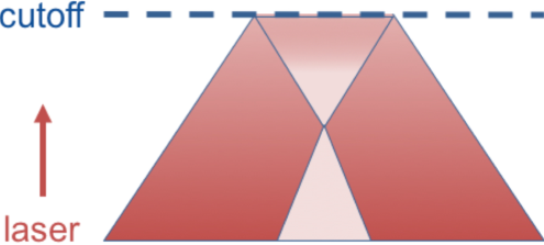
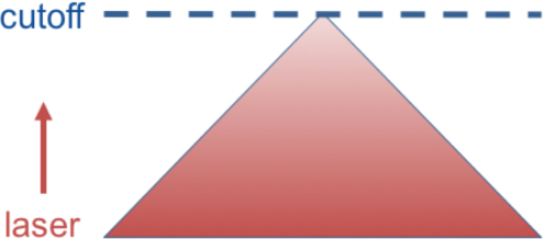
diverges in the geometrical-optics limit . This has consequences for setting intensity limiters for ray-tracing simulations near turning points. For example, a 351 nm wave incident on a plasma with 1 mm density scale length can potentially swell times higher than the Airy limiter often used [7]. That said, since a Gaussian-focused wave approaches a plane wave in the limit it must be the case that reduces to Ai when the focusing terms are negligible close to the turning point. The general morphology of Eq. 12 is given by the series of cartoons in Fig. 1; more detailed pictures of the field structure of are provided in Ref. [3].
4 Apertured field special case
Lastly, let us consider when the incident wavefield is passed through an aperture:
| (14) |
where is the arbitrary un-apertured wavefield and rect is the rectangular hat function of width . If the aperture width is made infinitesimally small, then one can show that Eq. 6 yields
| (15) |
Hence, an aperture drives all incident fields to an unfocused hyperbolic umbilic function. The journey of a given incident field to this common final state can be complicated, however. Specific examples for an incident plane and Gaussian-focused waves are given in Ref. [3].
5 Discussion & Conclusion
Here I have summarized a new description for general wavefields near turning points, illustrated with a number of simple examples. These results can be useful for developing improved reduced models for wave processes. For example, ECRH during the rampup phase on spherical tokamaks [8] will invariably encounter the critical focusing case as the cutoff layer surpasses the resonance layer; applying caustic-agnostic methods such as metaplectic geometrical optics [9, 10, 11, 12] to such ray-tracing simulations will ensure that the hyperbolic umbilic function is calculated correctly.
References
- [1] N. Lemos, W. A. Farmer, N. Izumi et al, Phys. Plasmas 29, 092704 (2022)
- [2] D. Turnbull, P. Michel, J. E. Ralph et al, Phys. Rev. Lett. 114, 125001 (2015)
- [3] N. A. Lopez, E. Kur, and D. J. Strozzi, Phys. Rev. E 107, 055204 (2023)
- [4] F. W. J. Olver, et al, NIST Handbook of Mathematical Functions (https://dlmf.nist.gov/)
- [5] T. Poston and I. Stewart, Catastrophe Theory & Its Applications (Dover, New York, 1996)
- [6] W. L. Kruer, The Physics of Laser Plasma Interactions (CRC Press, Boca Raton, 2003)
- [7] J. F. Myatt, R. K. Follett, J. G. Shaw et al, Phys. Plasmas 24, 056308 (2017)
- [8] N. A. Lopez and F. M. Poli, Plasma Phys. Control. Fusion 60, 065007 (2018)
- [9] N. A. Lopez and I. Y. Dodin, New J. Phys. 22, 083078 (2020)
- [10] N. A. Lopez and I. Y. Dodin, J. Opt. 23, 025601 (2021)
- [11] N. A. Lopez and I. Y. Dodin, Phys. Plasmas 29, 052111 (2022)
- [12] N. A. Lopez, Metaplectic Geometrical Optics, (Ph.D thesis, Princeton University, 2022), arXiv:2210.03188