New trends in quantum integrability: Recent experiments with ultracold atoms
Abstract
Over the past two decades quantum engineering has made significant advances in our ability to create genuine quantum many-body systems using ultracold atoms. In particular, some prototypical exactly solvable Yang-Baxter systems have been successfully realized allowing us to confront elegant and sophisticated exact solutions of these systems with their experimental counterparts. The new experimental developments show a variety of fundamental one-dimensional (1D) phenomena, ranging from the generalized hydrodynamics to dynamical fermionization, Tomonaga-Luttinger liquids, collective excitations, fractional exclusion statistics, quantum holonomy, spin-charge separation, competing orders with high spin symmetry and quantum impurity problems. This article briefly reviews these developments and provides rigorous understanding of those observed phenomena based on the exact solutions while highlighting the uniqueness of 1D quantum physics. The precision of atomic physics realizations of integrable many-body problems continues to inspire significant developments in mathematics and physics while at the same time offering the prospect to contribute to future quantum technology.
I I. Introduction
Exactly solvable models date back to 1931 when Bethe Bethe:1931 introduced a particular form of wave function to obtain eigenspectrum of one-dimensional (1D) Heisenberg spin chain. His seminal many-body wave function which consisted of a superposition of all possible plane waves was later called Bethe ansatz. However, it was more than 30 years after his work that the Bethe ansatz was further applied to other physics problems in 1D, including the Lieb-Liniger Bose gas Lieb-Liniger:1963 , the Yang-Gaudin Fermi gas Yang:1967 ; Gaudin:1967 , the 1D Hubbard model Lieb:1968 , the SU(N) Fermi gases Sutherland:1968 , the Kondo impurity problems Andrei:1980 ; Wiegmann:1980 ; Tsvelik:1983 ; Andrei:1983 and the Bardeen-Cooper-Schrieffer (BCS) pairing model BCS:1957 ; Richardson:1963 ; Dukelsky:2004 among others. For a long time these exactly solvable models were considered to be mathematical toy models despite they had inspired significant developments in both mathematics and physics.
However, this impression was changed dramatically since the realization of one-dimensional integrable models of ultracold atoms in labs in the last two decades. Consequently, the study of exactly solvable models saw a renewed interest, see for instance the reviews Cazalilla:2011 ; Guan:2013 ; Batchelor:2016 ; Mistakidis:2022 .
This breakthrough was a result of a series of spectacular advances in the experimental control and manipulation of ultracold atoms, involving the trapping and cooling of atomic particles to extremely low temperatures of few nano-Kelvin above the absolute zero Giorgini:2008 ; Lewenstein:2007 . It led to finding new phases of cold matter resulting from the effects of interactions, statistics and symmetries of many atoms which requires deep understanding of coherent and correlation nature of many interacting particles at a higher level of rigor.
The experimental realizations of 1D Bose and Fermi gases with tunable interaction and internal degrees of freedom between atoms have provided a remarkable testing ground for quantum integrable systems.
Strikingly different features of many-body effects result from quantum degeneracy, i.e. bosons with integer spin obey Bose-Einstein statistics, whereas fermions with half odd integer spin obey Fermi-Dirac statistics. However, interactions among such degenerate cold particles can dramatically change their behaviour, resulting in novel many-body phenomena, for example, superfluid, such as Bose-Einstein condensation (BEC), quantum liquid, criticality etc.
The observed results to date are seen to be in excellent agreement with predictions from the exactly solved models. Early on, the prototypical integrable model–the Lieb-Liniger Bose gas was realized to reveal ground state properties, local pair correlation Kinoshita:2004 ; Paredes:2004 ; Kinoshita:2005 . Subsequently, the Yang-Yang thermodynamics and quantum fluctuation in the model were observed Amerongen:2008 ; Armijo:2010 ; Jacqmin:2011 ; Stimming:2010 ; Armijo:2012 ; Vogler:2013 . Based on theoretical prediction of the fermionization in the Lieb-Liniger gas Astrakharchik:2005 ; Batchelor:2005 , the novel super Tonks-Girardeau gas-like state was experimentally realized in Haller:2009 ; Kao:2021 . Observation of the quantum degenerate spin-1/2 Fermi gas Moritz:2005 ; Liao:2010 ; Zurn:2012 ; Zurn:2013 ; Zurn:2013b ; Wenz:2013 ; Murmann:2015 ; Revelle:2016 and SU(N) Fermi gases Pagano:2014 ; Song:2020 are having high impact in ultracold atoms Wu:2003 ; Wu:2006 .
New trends in experiments with Yang-Baxter quantum integrability involve quantum criticality and Luttinger liquid Haller:2010 ; Fabbri:2015 ; Meinert:2015 ; Yang:2017 ; YangTL:2018 , quantum dynamics, thermalization, correlation Schweigler:2017 ; Prufer:2017 ; Wilson:2020 ; Sun:2021 ; Tang:2018 ; Erne:2018 . Very recently, the 1D Hubbard model Boll:2016 ; Hilker:2017 ; Vijayan:2020 ; Spar:2022 , 1D p-wave polarized fermions Chang:2020 ; Ahmed-Braun:2021 ; Jackson:2022 ; Venu:2022 , 1D matter wave breathers Yurovsk:2017 ; Luo:2020 ; Marchukov:2020 and emergent dynamical quasicondensation of hard-core bosons at finite momenta Vidmar:2015 also found their ways into the lab. As a result, the mathematical physics of Bethe ansatz integrable models has not only become testable in experiments with ultracold atoms but the experiments also provided impetus for many new developments of quantum integrability. For example, the realization of the quantum Newton cradle in the 1D Lieb-Liniger gas Kinoshita:2006 led to a new surge of study of integrable models. In particular, the experimental observation of the quantum Newton’s cradle Kinoshita:2006 raised a significant question for theory and experiment: can the evolution of isolated quantum integrable systems of many particles converge into its equilibrium Gibbs thermal state? Seeking for an understanding of such a subtlety of quantum dynamics of quantum integrable models leads to new developments of the Generalized Gibbs ensemble (GGE) Rigol:2007 ; Ilievski:2015 and generalized hydrodynamics (GHD) Castro:2016 ; Bertini:2016 , which have become a promising theme in theory and experiment with 1D ultracold atoms Langen:2015 ; Schemmer:2019 ; Malvania:2021 ; Berg:2016 ; Caux:2019 ; Nardis:2018 ; Bastianello:2019 ; Bastianello:2020 ; Ruggierro:2020 ; Doyon:2017 ; Fava:2021 ; Bastianello:2022 ; Bouchoule:2022 ; Moller:2022 ; Bertini:2022 ; Moller:2021 ; Li-Chen:2020 ; Cataldini:2021 .
Last but not least, the quantum walks of one magnon and magnon bound states in interacting bosons on 1D lattices Fukuhara:2013a ; Fukuhara:2013b , realization of 1D antiferromagnetic Heisenberg spin chain with ultracold spinor Bose gas Sun:2021 , quantum impurities Catani:2012 ; Meinert:2017 , fractional quantum statistics Zhang:2022 and spin-charge separation Senaratne:2021 open new frontiers in quantum technology.
II II. Exactly solved models in ultracold atoms
The study of Bethe ansatz solvable models flourished in the period from 1960s to 1990s in the mathematical physics communities in the world. A number of notable Bethe ansatz integrable models in a variety of fields of physics were solved at that time. In the last two decades, a considerable attention has been paid to the study of 1D exactly solved models due to unprecedented abilities in cooling and controlling cold atoms in low dimensions. The exact results of the integrable models provide deep insight into the quantum simulation and understanding of many known as yet unknown quantum phases of matter in ultracold atoms, condensed matter physics and quantum metrology. Here we first introduce several exactly solvable models which have provided rigorous understanding of fundamental many-body physics observed so far in low-dimensional ultracold atoms and will give further possibilities for exploring subtle quantum phenomena in 1D.
II.1 Lieb-Liniger Bose gas
The Hamiltonian of the Lieb-Liniger gas of particles with periodic boundary conditions in a length is given by Lieb-Liniger:1963
| (1) |
where is the mass of the bosons, is the coupling constant which is determined by the the 1D scattering length . The scattering length is given by Olshanii_PRL_1998 ; Dunjko_PRL_2001 ; Olshanii_PRL_2003 . In the above equation, the canonical quantum Bose fields satisfying the following commutation relations
Solving the Schrödinger equation reduces to the eigenvalue problem of the many-particles Hamiltonian
| (2) |
Here the effective coupling constant .
Following the Bethe ansatz Bethe:1931 the wave function is divided into domains according to the positions of the particles , where is the permutation of number set . The wave function can be written as . Considering the symmetry of bosonic statistics, all the in different domain should be the same, i.e., , where we use to denote the elements of the identity permutation, . Lieb and Liniger Lieb:1968 wrote the wave function for the model (2) as the superposition of plane waves
| (3) |
where denotes the permutation of number set with the pseudo-momenta s carried by the particles under periodic boundary conditions. They satisfy a set of Bethe ansatz equations, called the Lieb–Liniger equations
| (4) |
Here . For a given set of quasi-momenta , the total momentum and the energy of the system are obtained by
| (5) |
The fundamental physics of the model (2) are essentially determined by the wave function (3) and the Lieb–Liniger equations (4), see a review Jiang:2015 .
In 1969 C N Yang and C P Yang Yang-Yang:1969 published their seminal work on the thermodynamics of the Lieb-Liniger Bose gas. The thermodynamics of the Lieb-Liniger gas is determined from the minimization conditions of the Gibbs free energy in terms of the roots of the Bethe ansatz equations (4). In the thermodynamic limit, the Bethe ansatz equations (4) become
| (6) |
where and are respectively the particle and hole density distribution functions at finite temperatures. The Gibbs free energy per unit length is given by with the relation to the free energy . Here is the chemical potential, is the linear density, and is the entropy. The minimization condition with respect to particle density leads to the Yang-Yang thermodynamic Bethe ansatz (TBA) equation Yang-Yang:1969
| (7) |
which determines the thermodynamics of the system in the whole temperature regime through the Gibbs free energy per length, i.e.,
| (8) |
Thus other thermodynamic quantities can be obtained through thermodynamic relations, for example the particle density, entropy density, compressibility, specific heat are given by
| (9) |
In the above equation denotes the derivative respect to the potentials. Exact Bethe ansatz solution provides an analytical way to access to quantum critical behaviour of the system at finite temperatures Guan:2011 ; Jiang:2015 .
II.2 Yang-Gaudin model
1D models of Bethe ansatz solvable quantum gases have become an important subject of experiment, such as two-component spinor fermions and bosons as well as multi-component fermions. Models of this kind have rich internal degrees of freedom and high symmetries. In 1967, C N Yang Yang:1967 solved the 1D delta-function interacting Fermi gas wit the discovery of quantum integrability, i.e. the necessary condition for the Bethe ansatz solvability. This quantum integrability condition was referred to the factorization condition–the scattering matrix of a quantum many-body system can be factorized into a product of many two-body scattering matrices. At the same time, M Gaudin also rigorously derived the Bethe ansatz equations for the spin- Fermi gas for spin balance case Gaudin:1967 . Therefore, the 1D spin- Fermi gas is now called the Yang-Gaudin model. On the other hand, in 1972, R J Baxter Baxter:1972 independently found that a similar factorization relation also occurred as the conditions for commuting transfer matrices in 2D vertex models in statistical mechanics. Such a factorization condition is now known as the Yang-Baxter equation and becomes a significant key condition to quantum integrability.
The many-body Hamiltonian for the Yang-Gaudin model is given by Yang:1967 ; Gaudin:1967
| (10) |
describes fermions of the same mass with two internal spin states confined to a length interacting via a -function potential. In the above equation, prime denotes the exclusion of the interaction between two atoms with the same spin. Here we denoted the numbers of fermions in the two hyperfine levels and as and , respectively. The total number of fermions and the magnetization were denoted as and , respectively. The interaction strength is given by with , where is the effective 1D scattering length, see the discussion on the Hamiltonian of the Lieb-Liniger gas. For convenience, we also define a dimensionless interaction strength . Here the linear density is defined by ; meanwhile, for a repulsive interaction and for an attractive interaction, see review Guan:2013 .
C N Yang generalized Bethe’s wave function to the following many-body wave function of the spin- Fermi gas
| (11) |
for the domain . Where denote a set of unequal wave numbers and with indicate the spin coordinates. Both and are permutations of indices , i.e. and . The sum runs over all permutations and the coefficients of the exponentials are column vectors with each of the components representing a permutation . For determining the wave function associated with the irreducible representations of the permutation group and the irreducible representation of the Young tableau for different up- and down-spin fermions, C N Yang found a key condition for solvability, i.e., the two-body scattering matrix acting on three linear tensor spaces
| (12) |
satisfies the following cubic equation
| (13) |
which has been known as the Yang-Baxter equation Yang:1967 ; Baxter:1972 . It is worth mentioning that an experimental simulation of the Yang-Baxter equation itself through the linear quantum optics Zhang:2013 and the Nuclear Magnetic Resonance interferometric setup Vind:2016 has been performed. In the above equations, we denoted the operator , here is the permutation operator. The Yang-Baxter equation has found a profound legacy in both mathematics and physics, see review 1D-Hubbard ; Korepin ; Sutherland-book ; Takahashi-b ; Wang-book ; Guan:2013 .
Solving the eigenvalue problem of interacting particles (10) in a periodic box of length with the periodic boundary conditions, C N Yang obtained the Bethe ansatz equations for the Fermi gas Yang:1967
| (14) | |||
| (15) |
with and . Here is the number of atoms with down-spins. The energy eigenspectrum is given in terms of the quasimomenta of the fermions via . In the above equations (14) and (15), denoted spin rapidities. All quasimomenta are distinct and uniquely determine the wave function of model Eq.(11).
The fundamental physics of the model (10) can be obtained by solving the transcendental Bethe ansatz equations (14) and (15). Finding the solution of the Bethe ansatz equations (14) and (15) is extremely cumbersome. For a repulsive interaction, in the thermodynamic limit, i.e., , and is finite, the above Bethe ansatz equations can be written as the generalized Fredholm equations
| (16) | |||||
| (17) | |||||
The associated integration boundaries , are determined by the relations
| (18) |
where denotes the linear density, while is the density of spin-down fermions. In the above equations we introduced the quasimomentum distribution function and distribution function of the spin rapidity for the ground state.
The thermodynamics of the Yang-Gaudin model with a repulsive interaction was studied by C K Lai Lai:1971 ; Lai:1973 and M Takahashi Takahashi:1971 . In the same fashion as the derivation of the thermodynamics of the Lieb-Liniger Bose gas by C. N. Yang and C. P. Yang in 1969 Yang-Yang:1969 , M Takahashi Takahashi:1971 gave the thermodynamic Bethe ansatz equations for the repulsive Yang-Gaudin model
| (19) | |||||
| (20) | |||||
with . Here denotes the convolution, i.e. , and are the dressed energies for the charge and the length- spin strings, respectively, with ’s and ’s being the rapidities; and the function is given by
| (24) |
Where we denoted . The pressure is given by
| (25) |
from which all the thermal and magnetic quantities, as well as other relevant physical properties, such as Wilson ratio Guan:2013b and Grüneisen parameter Peng:2019 ; Yu:2020 , can be derived according to the standard statistical relations.
For a attractive interaction, i.e. , the root patterns of the BA equations (14) and (15) are significantly different from that of the model for . In this regime the quasimomenta of the fermions with different spins form two-body bound states Takahashi-a ; Gu-Yang ; Guan:2007 , leading to the existence of the Fulde-Ferrell-Larkin-Ovchinnikov (FFLO) pairing state Larkin1965 ; Fulde1964 ; Yang2001 . Here we will not discuss the attractive Yang-Gaudin model Orso:2007 ; Hu:2007 ; Guan:2007 ; Liu:2008 ; Zhao:2009 ; LeeGuan:2011 ; HeJS:2009 , a more detailed study of this model can be found in the review article Guan:2013 .
II.3 Multi-component Fermi gases with symmetry
It is shown that the fermionic alkaline-earth atoms display an exact spin symmetry with , where is the nuclear spin Cazalilla:2009 ; Gorshkov:2010 . For example, the experiment Taie:2010 for 171Yb dramatically realised the model of fermionic atoms with symmetry where electron spin decouples from its nuclear spin , and 87Sr atoms have symmetry XZhang2014S . These experimental developments have opened exciting opportunities to explore a wide range many-body phenomena such as spin and orbital magnetism Cappellini2014PRL ; Scazza2014NP , Kondo spin-exchange physics Nakagawa:2015 ; Zhang2015 and the one-dimensional (1D) Tomonaga-Luttinger liquid (TLL) Pagano:2014 etc. Such fermionic systems with enlarged spin symmetry are expected to display a remarkable diversity of new quantum phases and quantum critical phenomena due to the existence of multiple charge bound states Guan:2013 ; Wu:2006 . Here we do not wish to review the developments of Fermi gases in details. We prefer to briefly introduce the integrable Fermi gases with repulsive interactions.
We introduce the Hamiltonian of -component Fermi gas of particles with mass Sutherland:1968
| (26) |
where is the total spin of the -direction, and is the external magnetic field. In the above equation, the prime stands for the exclusion of the interaction between two atoms with the same spin. Here is the particle number in the hyperfine state . There are possible hyperfine states that the fermions can occupy. Again the interaction coupling constant is given by , and . Here is the effective scattering length in 1D. The Hamiltonian (26) has the symmetry of when the magnetic field is absent, where and are the symmetries of the charge and spin degrees of freedom, respectively.
Using Bethe’s hypothesis, B Sutherland exactly solved the model by giving the energy , and the Bethe ansatz equations
| (27) | |||
| (28) | |||
| (31) | |||
| (32) | |||
Here , denote the spin rapidities which are introduced to describe the motion of spin waves. The particle number in each spin state links to the quantum number via the relation and . For the repulsive interaction, i.e. , there is no charge bound state, whereas each branch of spin rapidities has complex roots
| (33) |
in the thermodynamic limit, which are now called spin wave bound states.
Following Yang-Yang’s grand canonical method Yang-Yang:1969 the thermodynamic Bethe ansatz equations for the Fermi gases (26) are given by Takahashi-b ; Guan:2013 ; Schlottmann:1997 ; Lee:2011 ; Jiang:2016
| (34) |
| (35) | |||||
| (36) | |||||
| (37) |
Where and are the dressed energies for the charge sector and for the branch in the spin sector, respectively and . As a convention used in the TBA equations, labels the length of the strings, labels the convolution integral and the integral kernels are given by
| (38) |
The pressure is given by
| (39) |
which serves as the equation of states for the repulsive Fermi gases.
The Bethe ansatz equations (27)-(32) and the thermodynamic Bethe ansatz equations (34)-(37) impose a big challenge in obtaining physical properties of the model Batchelor:2007 ; Schlottmann:1997 ; Lee:2011 ; Guan:2012a ; Guan:2012b ; Jiang:2016 ; Yang-You:2011 . At low temperature, the behaviour of the Fermi gases with a repulsive interaction is described by spin-charge separated conformal field theories of an effective Tomonaga-Luttinger liquid and an antiferromagnetic Heisenberg spin chain, see experiment observation Pagano:2014 . It was found Jiang:2016 ; Liu:2014 ; Schlottmann:1993 that the sound velocity of the Fermi gases in the large limit coincides with that for the spinless Bose gas, whereas the spin velocity for balance gases vanishes quickly as becomes large. This novel feature of 1D multi-component Fermi gases shows a strong suppression of the Fermi exclusion statistics by the commutativity feature among the -component fermions with different spin states in the Tomonaga-Luttinger liquid phase, which was for the first time proved by Yang and You Yang-You:2011 in 2011, and confirmed by Guan and coworkers Guan:2012b in 2012. This feature was recently demonstrated with ultracold atoms in 2D Song:2020 .
Moreover, the 1D multi-component Fermi gases exhibit significantly different features from usual interacting electrons, showing rich pairing phenomena in momentum space, see review Guan:2013 .
III III. Generalized hydrodynamics of integrable systems
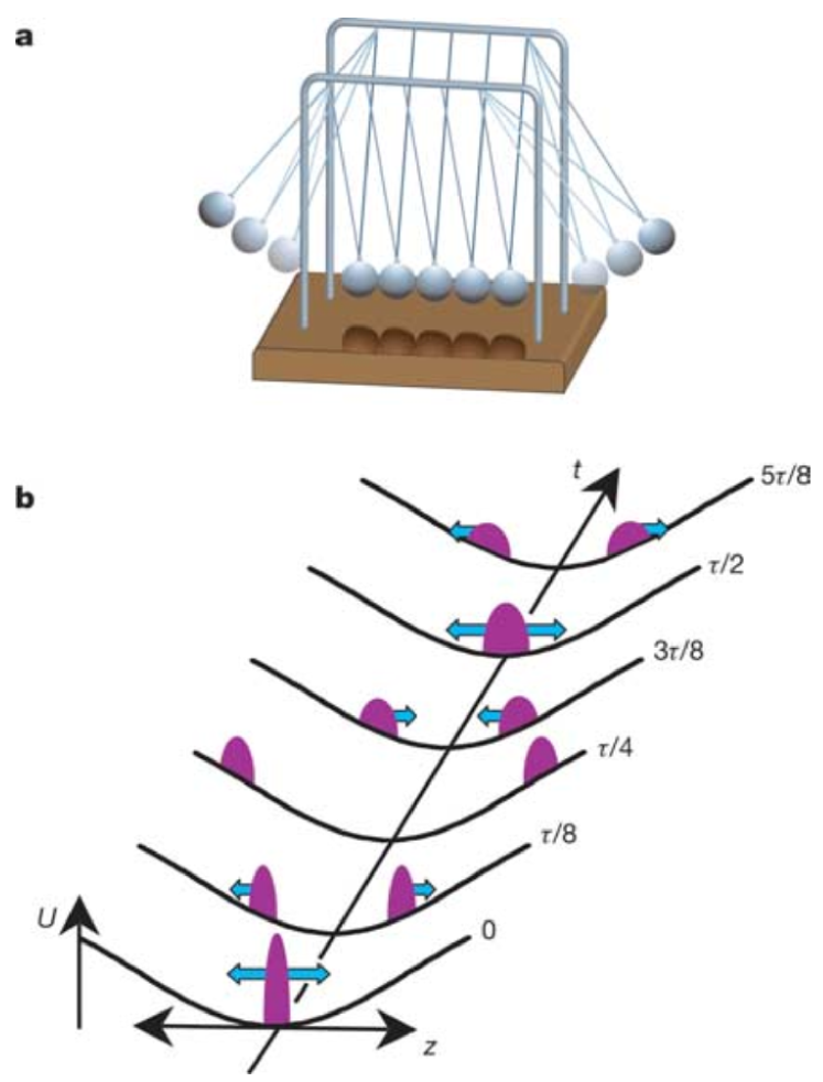
Dynamical properties of isolated many-body systems have been the central problem in quantum statistics for a long time. In the last decade, versatile dynamical properties of 1D integrable models have been demonstrated in the field of ultracold atoms. In 2006, D. Weiss’s group from the Pennsylvania State University demonstrated nonequilibrium behaviour of interacting Bose gas in a quasi-1D harmonic trap in their seminal paper Kinoshita:2006 , see Fig. 1. The clouds of quasi-1D trapped Bose gas in momentum space oscillate out-of-equilibrium for several dozens of ms that remarkably illustrated behaviour of quantum Newton’s cradle. The framework to describe such kind of dynamics of integrable models out-of-equilibrium has been mainly built on the GGE Rigol:2007 ; Ilievski:2015 and the GHD Castro:2016 ; Bertini:2016 with respect to an axial inhomogeneous trap Berg:2016 ; Caux:2019 ; Nardis:2018 ; Bastianello:2019 ; Bastianello:2020 ; Ruggierro:2020 ; Doyon:2017 ; Fava:2021 . Further demonstrations of the GHD were carried out by using a quantum chip setup and the quasi-1D trap of ultracold atoms Schemmer:2019 ; Malvania:2021 . So far, there have been a variety of theoretical methods for studying the Newton’s cradle-like dynamics of 1D systems out-of-equilibrium. Here we do not wish to review whole developments of the hydrodynamics. We will introduce the basic concepts of the GHD for later use in this paper. More detailed theory of the GHD can be seen in two nice lecture notes by B Doyon Doyon:2017-L ; Doyon:2020-L .
We recapitulate the GHD of the 1D integrable systems introduced in the references Castro:2016 ; Bertini:2016 . On the large scale, GHD is the classical hydrodynamics, and for both we need a local equilibrium approximation, namely a system displays a large scale motion which can be separated into many fluid cells, and all these cells are large enough to be macroscopic and small enough to be homogeneous comparing to the size of the system. The system can then be characterized by
| (40) |
where is the density matrix of an equilibrium state and is the position of the th fluid cell. In each cell, entropy maximisation occurs, i.e., reaching a local thermodynamic equilibrium.
On the other hand, for integrable systems with degrees of freedom, there are many local conserved quantities , called conserved charges, the fundamental objects for quantum integrability. An GGE state is a maximal entropy state and its density matrix is constrained by all the conserved quantities by Rigol:2007 ; Ilievski:2015
| (41) |
Thus an equilibrium state of integrable systems can be identified by the expectation values of all the conserved quantities , where , and s are the associated potentials. For an non-equilibrium state, under local time-space equilibrium approximation, integrable systems can be described by the distributions of all the conserved quantities , where and ,
| (42) |
Let us denote densities of conserved charges as a function of and . They determine the equilibrium state of fluid cells. In turn, the local potentials are determined too once the cells reach local time-space equilibrium. Subsequently, one can define the average values of local conserved charges and their corresponding currents via
| (43) | |||||
| (44) |
becoming the Gibbs average of local densities and currents under the time and coordinates dependent potentials, respectively.
According to the GHD approach, we assume that all the local conserved quantities satisfy the continuity equations
| (45) |
with . The density and current of the -th conserved quantity essentially describe variations of thermally average conservation laws at the Euler scale.
In order to build up the description of the GHD for integrable models, it is a useful way to express the charge densities in terms of the quasiparticle rapidity densities of the Bethe ansatz solvable models. Here we just formulate the conserved charge densities by the quasiparticle density for the Lieb-Liniger model, namely
where is the corresponding rapidity, and is one particle eigenvalue of -th conserved charge. For example, particle density , energy density and momentum density , etc. It is also very useful to introduce the state density and the quasiparticle occupation number Here the state density satisfies the Lieb-Liniger equation
| (46) |
which was given by Eq. (6). Here is the derivative of the momentum with respect to and is the integral kernel function. By properly choosing a linear space of pseudo-conserved charges as a function space spanned by all s, one can prove s form the generalized inverse temperatures or chemical potentials which are determined by the initial states. Following the unified notations used in Doyon:2017-L ; Doyon:2020-L , we may express the conserve charge as a linear function of the one particle eigenvalue . We define the one-particle eigenvalue of , thus the quasiparticle occupation number can be given by the GGE states
| (47) | |||||
| (48) |
Based on the analysis given in Castro:2016 , the energy, momentum and currents can be formally denoted as functions of ,
| (49) |
Here and are the quasi-particle density and current spectral density, respectively. We note that for the Lieb-Liniger model, there is no internal degree of freedom. Thus the current spectral density can be given by
| (50) |
see Castro:2016 ; Bertini:2016 . It turns out that
| (51) |
where and are the energy and momentum of quasiparticles in the rapidity space. This equation can be rewritten as
| (52) |
where the group velocity . In these equations of states, all conserved quantities can be obtained by the quasiparticle densities , i.e.
here the dressing operation is defined
| (53) |
In the above equations, the following notations were used
Following the argument on the completeness of the set of functions s Castro:2016 ; Doyon:2017-L ; Doyon:2020-L , we have
| (54) |
Thus the GHD equations can be expressed as in different forms, for example
| (55) |
Here the von Neumann entropy of local fluid cell GGE states is defined by
Recently, more subtle GHD for the systems with inhomogeneous trapping potentials, quantum fluctuations and diffusion were studied theoretically Berg:2016 ; Caux:2019 ; Nardis:2018 ; Bastianello:2019 ; Bastianello:2020 ; Ruggierro:2020 ; Doyon:2017 ; Fava:2021 ; Bastianello:2022 ; Bouchoule:2022 ; Moller:2022 ; Bertini:2022 ; Scopa:2021 and experimentally Schemmer:2019 ; Malvania:2021 ; Moller:2021 ; Li-Chen:2020 ; Cataldini:2021 .
IV IV. Experiments with quantum integrability
In quasi-1D ultracold atomic experiment, the particles are tightly confined in two transverse directions and weakly confined in the axial direction. The transverse excitations are fully suppressed by the tight confinements. Thus the atoms in these waveguides can be effectively characterised by a quasi-1D system Olshanii_PRL_1998 ; Dunjko_PRL_2001 ; Olshanii_PRL_2003 . In such a way, these 1D many-body systems ultimately relate to the integrable models of interacting bosons and fermions. We arguably say that the Lieb-Liniger gas is the most studied exactly solvable model in terms of ultracold atoms, see review Cazalilla:2011 ; Guan:2013 ; Mistakidis:2022 . Particularly striking features involved the measurements of Lieb-Liniger gas Lieb-Liniger:1963 were seen in a variety of physics from ground state properties Kinoshita:2004 ; Paredes:2004 ; Kinoshita:2005 to the thermodynamics Amerongen:2008 ; Armijo:2010 ; Jacqmin:2011 ; Stimming:2010 ; Armijo:2012 ; Vogler:2013 ; Haller:2009 ; Kao:2021 , quantum dynamics Langen:2015 ; Schemmer:2019 ; Malvania:2021 ; Kinoshita:2006 ; Hofferberth:2007 ; Ronzheimer:2013 ; Schweigler:2017 ; Prufer:2017 , the quantum GHD Schemmer:2019 ; Malvania:2021 , quantum criticality and Luttinger liquid Haller:2010 ; Meinert:2015 ; Yang:2017 . On the other hand, the Yang-Gaudin model Yang:1967 ; Gaudin:1967 and the 1D SU(N) Fermi gases Sutherland:1968 have also become a paradigm of ultracold fermionic atoms in 1D Liao:2010 ; Zurn:2012 ; Zurn:2013 ; Zurn:2013b ; Wenz:2013 ; Murmann:2015 ; Revelle:2016 ; Pagano:2014 ; Song:2020 . In this section we would like to review briefly several recent experiments on quantum integrable models.
IV.1 IV.1. Quantum Newton’s Cradle
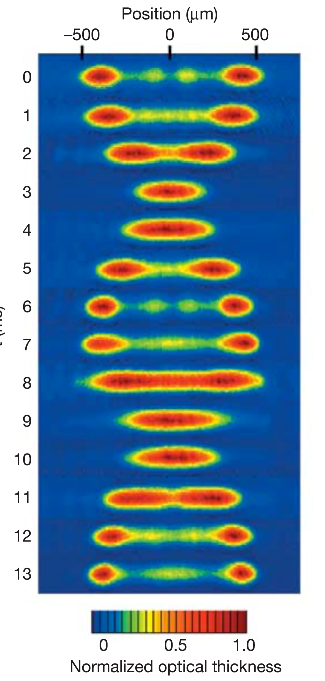
The understanding of the quantum Newton’s cradle observed in Kinoshita:2006 has been received significant theoretical attention Berg:2016 ; Caux:2019 ; Nardis:2018 ; Bastianello:2019 ; Bastianello:2020 ; Ruggierro:2020 ; Doyon:2017 ; Fava:2021 . In these works a key point was made that one can describe the motion of quasiparticles in the quasi-1D trapped gases after a sudden change of the longitudinal potential. In the experiment Kinoshita:2006 , a 2D array of 1D tubes were made by a tight transverse confinement and a crossed dipole trap providing weak axial trapping. They measured the density profile after a release of the 1D trapping potential. The 1D spatial distribution corresponds to the momentum distribution after a time-of-flight (TOF). They observed a separation of two clouds in the ensemble of quasi-1D trapped Bose gases of 87Rb atoms over the thousands of collisions between the clouds. In their experimental setting, each tube contained to atoms in the 2D arrays. They integrated the images inverse to the tubes to get 1D special distributions of momentum , see Fig. 2. From the distribution in space at different times, oscillations of two separated clouds showed a nearly Newton’s cradle dynamics from time to time in each measurement.
The quantum Newton’s cradle observed in Kinoshita:2006 received an immediate theoretical attention Rigol:2007 ; Ilievski:2015 . In a theoretical paper Caux:2019 , the authors gave a quantitative demonstration of the emergence of the quantum dynamics of Newton’s cradle through numerical study of the time evolution of the quasi-1D trapped Lieb-Liniger gas with an initial state
| (56) |
Where the distribution function of quasiparticles is space-time dependent. The momentum of quasiparticle was kicked by with equal probability. The gas was imparted into two clouds which had a strong inter-cloud repulsion. Based on such quantum Newton’s cradle setup, the GHD equation was given by
| (57) |
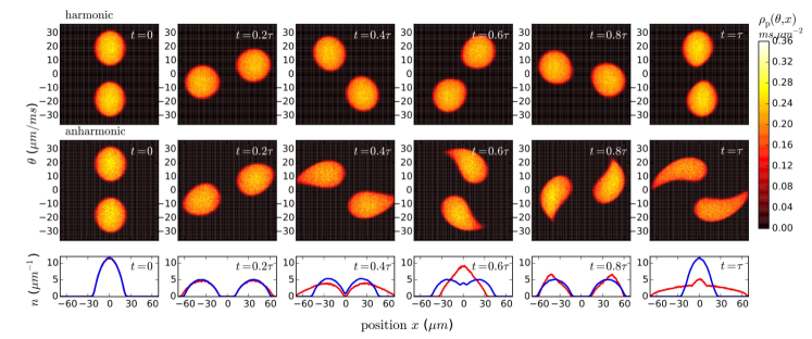
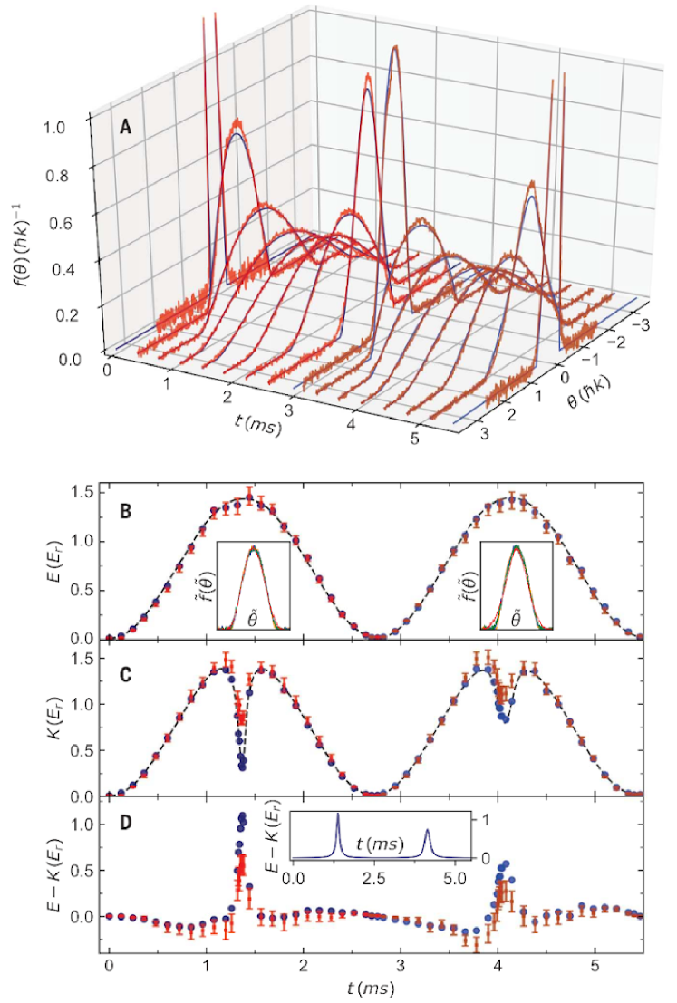
that remarkably gave the similar Newton’s cradle dynamics as observed in Kinoshita:2006 . In the above equation (57), denotes the trapping potential. In Fig. 3, they showed evolution of the density of quasiparticles determined by Eq.(57) with the initial state (56) using the experimental setting given in Kinoshita:2006 . In Fig. 3 (bottom panel), the boson density profiles show a dramatical oscillation of the two atomic clouds which were initially imparted by different kicks. The real-space density profile with was directly red off from the quasimomentum distribution function of quasi-particles . The two blobs, which are separated in momentum space, evolve around the origin of phase space. Thus the GHD provided a full evolving phase-space () distributions of quasiparticles associated with the Lieb-Liniger model, see upper panels in Fig. 3. Here it was showed that the GHD approach describes well slow variations of densities of particles, energy and higher conserved quantities on Euler scale. A more detailed theoretical analysis was given in Caux:2019 .
IV.2 IV.2. Generalized Hydrodynamics in Lieb-Liniger Model
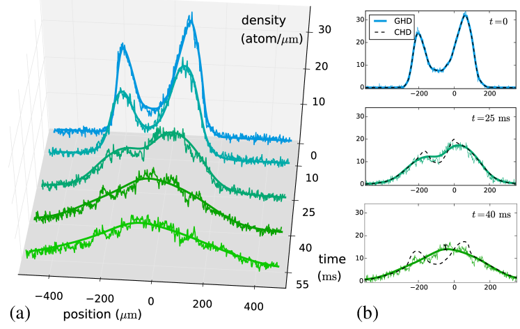
In 2019, Schemmer et al. presented a beautiful study on the emergence of the GHD of integrable Lieb-Liniger gas on an atom chip Schemmer:2019 . They observed time evolution of the in situ density profiles of a single 1D cloud of 87Rb atoms trapped on an atom chip for several different changes of longitudinal initial potentials. The experimental data were compared with the GHD of trapped gas Eq. (57) and the conventional hydrodynamics (CHD) determined by the following equations
| (58) |
here the energy is denoted by , the energy per particle was denoted by , denoted the mass of particles, and denoted the velocity, particle density and pressure, respectively. They are the functions of time and space . The pressure can be obtained from the thermodynamics Bethe ansatz equations (7). Again, denoted the trapping potential. Building on the GHD description of quantum quench dynamics in the quasi-1D trapped gases, they found a good agreement between the experimental results and theoretical simulations. In contrast, the CHD description either works or not for 1D integrable models depending solely on smoothness of the initial trapping potential. From the in situ density profiles they found that both GHD and CHD describe well longitudinal expansion dynamics from a harmonic trap of a 1D cloud of ultracold 87Rb atoms. However, the expansion dynamics from a double well potential further confirmed the validity of GHD for the integrable model. It appeared to be an obvious discrepancy between the experimental in situ density profiles and theoretical simulation from the CHD, see Fig. 4. They demonstrated that the GHD is applicable to all interacting regimes in the quench dynamics of integrable Lieb-Liniger Bose gas on the Euler scale.
In 2021, D. S. Weiss’s group Malvania:2021 further demonstrated the GHD of the quasi-1D trapped Bose gas in both the strong and intermediate coupling regimes. They measured the rapidity distributions in several ways by changing the quench potentials. Such changes of quench were still small enough so that the transverse excitations were fully suppressed. The key result of their paper was the validation of the GHD via the (per particle) rapidity momentum distribution , the ( per particle) rapidity energy , the (per particle) kinetic energy and (per particle) interaction energy , which are given by the Bethe ansatz rapidity
| (59) | |||||
| (60) | |||||
| (61) | |||||
| (62) |
where is the local density of quasi-particles in the -th tube, the sum runs over all tubes in the 2D arrays. In each fluid cell the rapidity density satisfies the local rapidity Bethe ansatz equation (46). The above formula can be derived in a straightforward way via the Bethe ansatz equation. Considering zero entropy limit, the measured evolutions of the above quantities in a sudden quench of the interaction from an initial state were seen in agreement with the prediction of the GHD theory, see Fig. 5.
From the above discussion, we see that the isolated integrable systems in general do not thermalize during evolution from an initial quench. The thermalization near integrability in the dipolar quantum Newton’s cradle was recently studied Tang:2018 . In this system, the 1D Bose gas of Dysprosium atoms with a strong magnetic dipole-dipole interaction was created by tuning the strength of the integrability-breaking perturbation and nearly integrability. They found a strong evidence for thermalization close to a strongly interacting integrable point occurred followed by near exponential thermalization. The measured thermalization rate is consistent with theoretical simulation. Integrable and non-integrable quantum systems of ultracold atoms with tunable interactions open a new venue to study thermalization and thermodynamics in and out-of-equilibrium.
IV.3 IV.3. Dynamical Fermionization
On the other hand, the Bose-Fermi mapping mechanism Girardeau:1960 ; Girardeau:1965 suggests that the physical properties like density profile, the thermodynamical properties and the density and density correlation are the same for both the ideal Fermi gas and the homogeneous 1D Tonks-Girardeau Bose gas. However, the physical quantities related to the one-body density matrix with off-diagonal elements, consequently the momentum distribution for the Tonks-Girardeau Bose gas significantly differ from the one for the ideal Fermi gas. This is mainly because of the quantum statistics play a significant role in correlations. The dynamics of the Tonks-Girardeau Bose gas Minguzzi:2005 ; Rigol:2005 led to the notion of dynamical fermionization. The dynamical fermionization of the 1D Tonks-Girardeau Bose gas reveals the typical expansion dynamics produced by the many-body wave function Lyer:2012 ; Buljan:2008 ; Campbell:2015 .
The strongly interacting bosonic Tonks-Girardeau gas was initially trapped in harmonic potential. After a sudden release of the axial confinement, the momentum distribution of the gas rapidly evolves to that of the ideal Fermi gas in the initial trap. This phenomenon Minguzzi:2005 ; Rigol:2005 is now referred to the dynamical fermionization. It has been theoretically demonstrated for several integrable models of ultracold atoms, such as 1D Bose gas Bolech:2012 ; Campbell:2015 ; Xu:2017 , 1D anyon gas del-Campo:2008 , 1D spinor Bose gas Alam:2021 , and 1D Bose-Fermi mixture and anyons Patu:2021 ; Piroli:2017 . Now it is well established that the wave function of the Lieb-Liniger gas (2) with an infinity strong repulsion can be written in terms of the one of the ideal fermions with the antisymmetric function in the same potential, referred as Bose-Fermi mapping Girardeau:1965 ; Girardeau:1960 . In a 1D harmonic trap with a time dependent trapping frequency and let , the many-body wave function of the the Tonk-Girardeau gas is given by
| (63) |
where is an antisymmetric function and the non-interacting fermion wave function is given by
| (64) |
The single-particle wave function can be obtained by solving the time-dependent Schrödinger equation with the following solution
| (65) |
where is the energy of the th single-particle eigenstate of the initial harmonic trap, the scaling parameter obeys the second differential equation with the initial conditions and . While the time scaling parameter , and is the wave function of the 1D harmonic oscillator with frequency and energy ,
Then the many-body wave function (63) can be given explicitly by
| (66) | |||||
where . Using this many-body wave function, the one-body density matrix can be calculated analytically and numerically, namely,
| (67) | |||
The time evolution of the momentum distribution is given by
| (68) |
Thus the expansion or quench dynamics of the 1D strongly interacting Bose gas can be studied by switching off the axial confinement potential or suddenly changing the trapping frequency. The quench dynamics of the 1D Bose gas with an arbitrary interaction strength was studied by D Iyer and N Andrei in Lyer:2012 . They showed that for any value of the interaction strength, as long as it is repulsive, the evolution of the system in a long time asymptotically approaches to the one of the hard core bosons at . Such dynamical fermionization is due to the structure of the two-body -matrix. The momenta integration contours in the wave function of Yudson representation are determined by the interaction. The interacting strength can be rescaled by the time, i.e. in the evolved wave function. The coupling constant effectively evolves with time. In the long time limit, the time rescaled scattering matrix , so that the asymptotic wave function of the bosons was represented by the one of the free fermions Lyer:2012 by using the stationary phase approximation. Thus the repulsively interacting bosons turn into fermions as time evolves in a long time Buljan:2008 ; Campbell:2015 . The fermionization also occurs in 1D lattice model of bosons and interacting anyons Piroli:2017 .
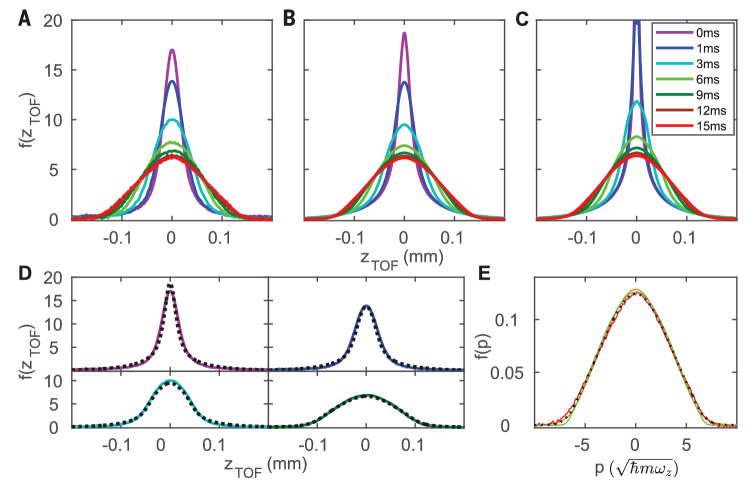
Following theoretical work Minguzzi:2005 ; Rigol:2005 ; Bolech:2012 ; Campbell:2015 ; Xu:2017 , the observation of the dynamical fermionization was carried out in Wilson:2020 . In this experiment, it was remarkable to observe that the momentum distribution of the Tonks-Girardeau gas evolved rapidly to the one of the ideal Fermi gas after an expansion in 1D, see Fig. 6. In this experimental setting, the interaction between the atoms was negligible upon expansion in the flat axial potential. The time-of-flight expansion profiles are in good agreement with the theoretical prediction for the Tonks-Girardeau gas as discussed above. At the evolution time ms, the Tonks-Girardeau gas rapidity distribution is the same as the momentum distribution of the ideal Fermi gas. The control capability to measure the momentum and rapidity distributions allow to further investigate more subtle quantum transport properties and diffusion in 1D quantum atomic gases.
IV.4 IV.4. Excitations and quantum Holonomy in Lieb-Liniger Gases
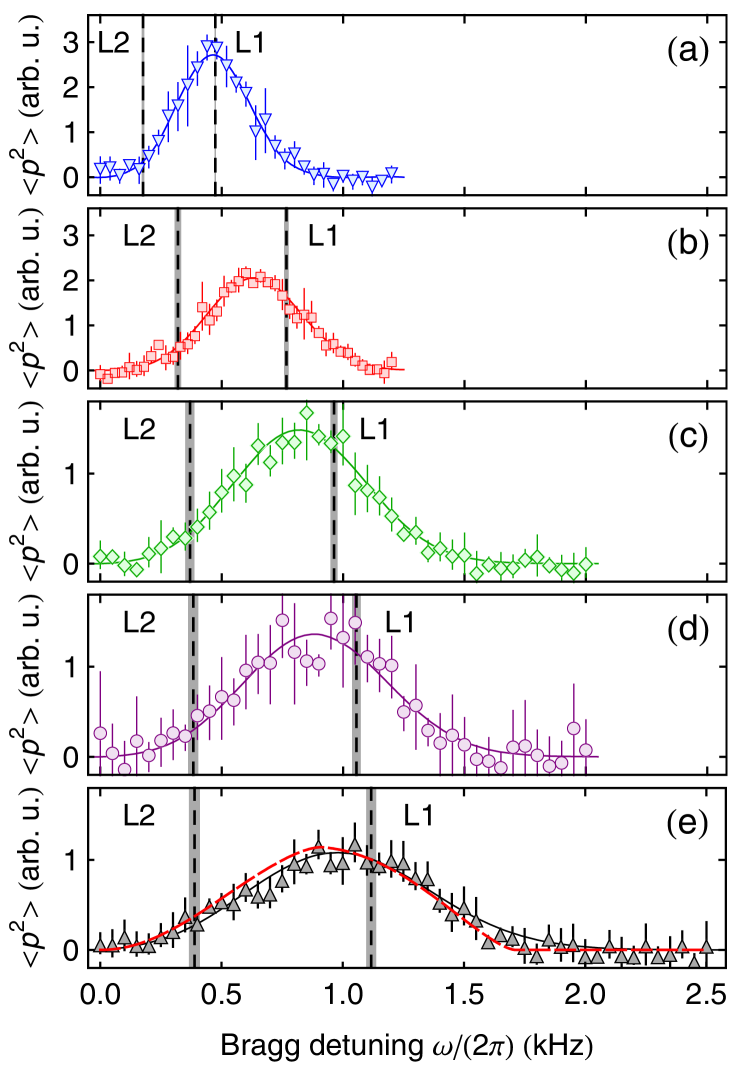
Elementary excitations: The Lieb-Liniger model Lieb-Liniger:1963 has been extensively studied in literature, see a review Cazalilla:2011 . In the last two decades this model has provided an unpreceedent ground for experimental investigation of a wide range of many-body phenomena, see introduction part. Regarding the low energy physics of the Lieb-Liniger gas, experimental observations of collective excitations in the Lieb-Liniger gases have been achieved in Fabbri:2015 ; Meinert:2015 . In the paper Meinert:2015 , by using the Bragg spectroscopy, the excitations for the quasi-1D trapped gases of Cesium atoms with tunable interaction strength were studied. An ensemble of independent 1D tubes was created by anisotropic confinements. The scattering length was tunable via a broad Feshbach resonance. The measured Bragg signal for a fixed value of momentum (about the mean value of ) was compared with the dynamical structure factor (DSF) at finite temperatures, i.e. . In this setting, the Luttinger liquid prediction on the DSF for the linear dispersion was not enough. They observed a clear broadening of the DSF peaks due to the Lieb-Liniger Type I (particle excitation ) and Type II (hole excitation ) excitations, see Fig. 7. The broadening signature for both excitations was revealed from the Bragg signal. In the figures (a)-(e), the broadening of the DSF spectral shape mainly came along with increasing the interaction strength. In particular, for the Tonks-Girardeau regime in Fig. 7(e), the experimental signals agree with the theoretical simulation with accounting for the effects of the inhomogeneous density distribution in each tube and the density distribution averaged over the ensemble of tubes at a temperature. The DSF was evaluated at finite temperature via the Bethe Ansatz-based numerical method, see Meinert:2015 . For low temperatures, the spectra showed a band width between the Lieb-Liniger Type I and Type II excitations. However, the band curvature effect in the DSF signal was not directly examined yet in this paper.
The temperature played an important role through the DSF and the inhomogeneous density distributions along the tubes in the theoretical simulation. This experiment opened to study low energy excitations for the integrability-based quantum systems of ultracold atoms.
Quantum holonomy: Stable highly excited states of interacting systems are extremely important in both theory and experiment. Such a metastable state can exist in the strong interacting bosons in 1D, referred to the super Tonks-Girardeau gas, which was predicted theoretically by Astrakharchik et al. Astrakharchik:2005 using Monte Carlo simulations and later by Batchelor, Guan and collaborators using the integrable interacting Bose gas with attractive interactions Batchelor:2005 . In a surprising experiment, Haller et al. Haller:2009 made a breakthrough by observing the stable highly excited gas-like state–the super Tonks-Girardeau gas in the strongly attractive regime of bosonic Cesium atoms. This observation has improved our understanding of quantum dynamics in many-body physics Chen:2010a ; Chen:2010b ; Yonezawa:2013 ; Tang:2018 . A physical intuition for the super Tonks-Girardeau gas is its metastable gas-like state with a stronger Fermi-like pressure than for free fermions which prevents a collapse of atoms in the strongly attractive interaction regime Chen:2010a ; Panfil:2014 ; Kormos:2011 ; Girardeau:2009 . From the Bethe ansatz, we observe that the energy at the limits is analytic, where the compressibility given by
| (69) |
is alway positive. Therefore such state is stable against collapse in the strongly attractive regime, even for the whole attractive regime. The energy of the super Tonks-Girardeau state can be increased smoothly when the attraction is ramped down to the noninteracting limit. A next cycle with an energy pumping can be repeated over the last cycle. This phenomenon is now called quantum holonomy Yonezawa:2013 .
Such exotic quantum holonomy was surprisingly demonstrated in a recent experiment did by B L Lev’s group in Stanford University Kao:2021 using the 1D Bose gas of dysprosium atoms with dipole-dipole interactions. The relevant Hamiltonian is given by
| (70) | |||||
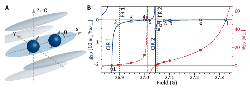
where is tunable by controlling the confine-induced-resonance. The dipole-dipole interaction essentially depends on the atomic dipole aligned angle by applying an external magnetic field to polarize dipoles through the scale factor , see Fig. 8. In the absence of the dipole-dipole interaction, the model (70) reduces to the Lieb-Liniger model (2). In this experiment, two cycles of quantum holonomy were demonstrated through tuning the interaction strength . The ensemble comprises an array of about 1D optical traps with about atoms per tube from the edge to the central tubes.
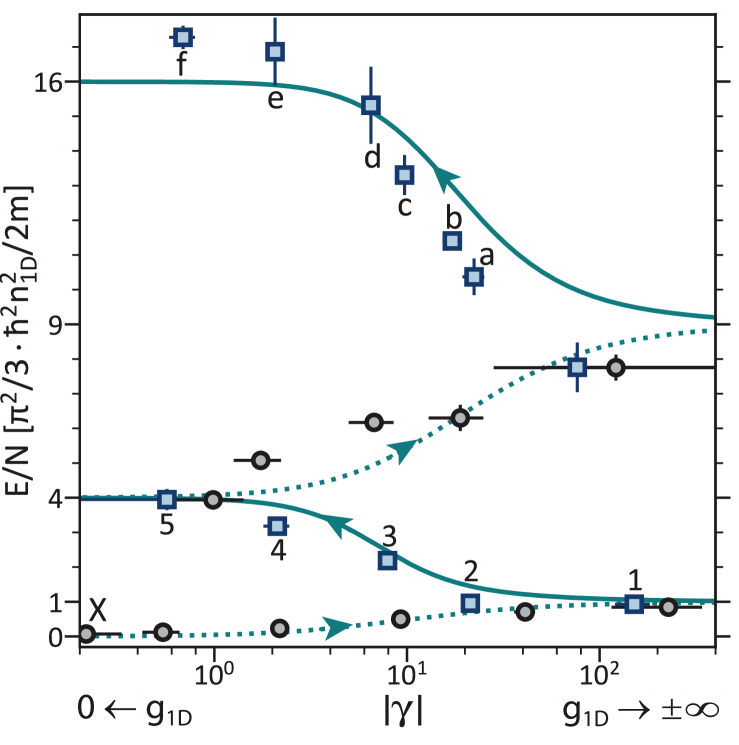
This experiment elegantly created a hierarchy quantum pumping by cyclically changing the short range interacting in the quasi-1D trapped Bose gas (70) for a fixed angle , see Fig. 9, where the per particle energy against the dimensionless interaction strength was measured through time-of-flight images. The authors demonstrated that the energy of the first cycle Tonks-Girardeau gas at the positive infinite repulsion limit is identical to the one of the second cycle super Tonks-Girardeau gas at the negative infinite repulsion limit. In contrast to the previous experiment with Cesium atoms by Haller et al. Haller:2009 , the dipole-dipole interaction at the ”magic” angle can stablize the super Tonks-Girardeau state at finitely strong attractions. Here the dipole-dipole interaction breaks the quantum integrability. However, such quantum holonomy does not seem to restrict to the integrable model. We would like to remark that this quantum holonomy can occur in 1D Bose gases because a full fermionization of interacting bosons at infinite strong interaction limit happens only in 1D. So that such highly excited states may analytically connect to the non-interaction limit. Nevertheless, the super Tonks-Girardeau states can occur in 1D interacting bosons and fermions, and p-wave interacting Fermi gases Yin:2011 ; Imambekov:2010 .
IV.5 IV.5. Luttinger liquids and Quantum criticality in Lieb-Liniger Gases
In 2011, Guan and Batchelor Guan:2011 calculated universal scaling functions of thermodynamics of the Lieb-Liniger Bose gas. The scaling behaviour of the thermodynamics of such an interacting Bose gas can be used to map out the criticality of the 1D model of ultracold atoms in experiment. The expression for the equation of state allows the exploration of Tomonaga-Luttinger liquid physics and quantum criticality in an arguably simple quantum system, see discussion of Lieb-Liniger Bose gas in Section II. At zero temperature, a quantum transition from vacuum to the TLL occurs when the chemical potential approaches to the critical point . The equation of the state is given by the universal scaling form of the density
| (71) |
where the background density in the limit . The scaling function reads off the dynamic critical exponent , and the correlation length exponent . The universal scaling functions of compressibility and specific heat are given by
| (72) | |||||
where the regular parts for the system in low temperature limit and the scaling functions and .
The low-lying excitations present the phonon dispersion in the long-wavelength limit, i.e. . In this limit, the following effective Hamiltonian Haldane:1981 ; Giamarchi-book
| (73) |
essentially describes the low-energy physics of the Lieb–Liniger gas, where the canonical momenta conjugate to the phase obeying the standard Bose commutation relations . is proportional to the density fluctuations. In this effective Hamiltonian, fixes the energy for the change of density. From the Bosonization approach, the leading order of one-particle correlation is uniquely determined by the Luttinger parameter . The Luttinger parameter is given by the ratio of sound velocity to stiffness, namely,
| (74) |
where is the sound velocity and is the stiffness. They are defined by
| (75) |
In the TLL phase, the momentum distribution is given by Cazalilla:2004
| (76) |
where is a -dependent parameter, and is the phase correlation length, see Cazalilla:2004 .
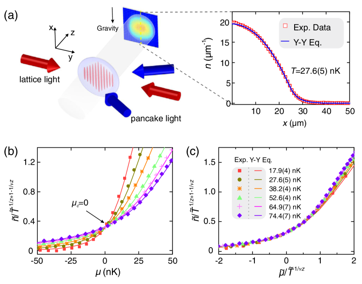
In a recent paper Yang:2017 , the quantum criticality and Luttinger liquid behaviour of the quasi-1D trapped ultracold 87Rb atoms were measured by in situ absorption imaging. In contrast to the usual 3D lattice arrays of 1D tubes, in this experiment, the density profiles were obtained by in situ absorption imaging of single tubes on a single 2D layer. The density and other thermodynamic scaling laws were obtained at different temperatures and chemical potentials by using a high-resolution microscope. Fig. 10 shows the experimental setting and the critical scaling of the density, see Yang:2017 . Here the dimensionless density was the function of dimensionless chemical potential and dimensionless temperature with . The intersection and collapse of density showed in (b) and (c) in the Fig. 10 confirmed the universal scaling law (71).
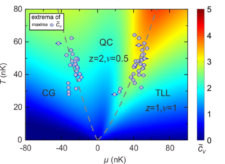
In Fig. 11, the universal phase diagram of criticality was obtained from the measurement of the specific heat in plane.
It was found that two crossover branches significantly distinguished the quantum critical regime from the classical gas (CG) and the TLL phase.
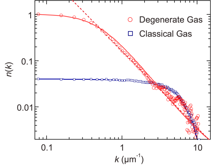
The measured double-peak structure of the specific heat (filled dots) coincides with the theoretical prediction (dashed lines) based on the TBA equation (7), see Fig. 11 (a). In figure (b), the measured momentum distribution at low temperature shows the power-law behavior, confirming the existence of the TLL.
In particular, the momentum distribution in logarithmic scale had the asymptotic power-law decay with the slope at large momenta (), see Yang:2017 .
Indeed, the experimental result agrees well with the theoretical prediction Cazalilla:2004 .
A remark made on the determination of the TLL in this Lieb-Liniger gas Yang:2017 and the arrays of Josephson junction Cedergren:2017 by T. Giamarchi Giamarchi:2017 is very inspiring:
“By providing a remarkable experimental demonstration of several so-far-elusive aspects of TLL theory, these two new studies confirm that TLL theory now plays the same key role in 1D systems that Fermi-liquid theory plays in our understanding of 2D and 3D condensed-matter systems. Without a doubt, this research will open new chapters in the TLL field by inspiring studies that examine how other perturbations (coupling between different 1D chains, spin-orbit coupling, and the like) can lead to novel and potentially exotic states in 1D materials.”
IV.6 IV.6. Can Quantum Statistics Be Fractional?
The Bose-Einstein and Fermi-Dirac statistics play a key role in modern quantum statistical mechanics. Now it is well established that they are not the only possible forms of quantum statistics Khare:2005 , for example, anyonic statistics can occur in excitations in 2D electronic systems, see early studies Leinaas:1997 ; Wilczek:1982 ; Arovas:1984 ; Laughlin:1988 . In this regard, a fractional exclusion statistics (FES) was introduced by F D M Haldane in 1991 Haldane:1991 . By counting the Hilbert space dimensionality for available single-particle states in a quantum system, the number of the available states (holes) of species decreases as particles ( ) of species are added to the system via
| (77) |
where the FES parameter is independent of the particle numbers , but essentially depends on the species and . Now it is called Haldane’s mutual FES. After Haldane’s work Haldane:1991 , Y S Wu Wu:1994 and other physicists Ha:1994 ; Isakov:1994 further formulated the Haldane’s FES. For a non-mutual FES, the parameter . It is obvious that the Bose-Einstein and Fermi-Dirac statistics correspond to the non-mutual FES with and , respectively. The FES has been used for the study of macroscopic properties in several 1D systems, including Calogero-Sutherland model of particles interacting through a potential Calogero:1969 ; Sutherland:1969 , the Lieb-Liniger Bose gases Bernard:1995 , and anyonic gases with delta-function interaction Kundu:1999 ; Batchelor:2006 .
On the other hand, critical phenomena in nature are ubiquitous. The quantum criticality of the Lieb-Liniger gas which was observed in Yang:2017 reveals a generic feature of continuous phase transition in interacting many-body systems. This feature can be commonly found in other systems, like 1D Heisenberg spin chain HeF:2017 as well as higher dimensional quantum systems Zhang:2012 ; Hung:2011 . Here we ventured to ask if universal nature of quantum criticality can exist beyond the scaling functions and renormalization sense? In a recent paper Zhang:2022 , based on exact solutions, quantum Monte Carlo simulations, and experiments, Zhang et al. demonstrated that macroscopic physical properties of 1D and 2D Bose gases at quantum criticality can be determined by a simple non-mutual FES.
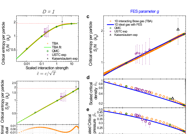
The FES has a long history of intensive studies, but its experimental realization in physical systems is very rare. Zhang et al. Zhang:2022 found that the non-mutual FES depicts the particle-hole symmetry breaking in 1D and 2D interacting Bose gases at a quantum critical point, see Fig. 12. In fact, in the vicinity of a quantum critical point, the system is strongly correlated with large characteristic lengths in real space. Thus in momentum space, the quasi-momentum cells become decoupled into nearly independent cells in which the densities of holes and particles satisfy the following relation
| (78) |
where is the bare dimensionality of states in the unit cell of phase-space for a -dimensional system. This form of particle-hole excitations can be found precisely from the Bethe ansatz equations for the Lieb-Liniger model Batchelor:2007b . It is obvious that particle-hole symmetry is broken in Eq. (78).
The physical properties of the system can be calculated through the simple distribution function of ideal particle with a non-mutual FES
| (79) |
Here and denoted the chemical potential and temperature. Moreover, the number density and energy density are given by and , where the density of states per volume is given by in 1D and for 2D non-relativistic particles. It is surprising to find that a simple one-to-one correspondence between the interaction strength in the quantum many-body systems and the statistical parameter can be given by
| (80) |
where is the maximum statistic parameter for the model with an infinitely strong interaction. The transformed interaction parameter is given by . Here the dimensionless interaction strength is given by for 1D Lieb-Liniger gas and is constant. They found the critical entropy per particle had a power-law dependence on the transformed parameter via , here , and for the Lieb-Liniger model. The overall good agreement with existing experimental data Vogler:2013 ; Yang:2017 , thermodynamic Bethe ansatz solution (7) and QMC simulation for the thermal properties: critical entropy per particle, dimensionless density and pressure was observed in Fig. 12. It held true for the 2D Bose gas, see a detailed analysis in Zhang:2022 . This research raises the question: can macroscopic thermodynamic properties be determined by the non-mutual FES which is described by interaction-induced particle-hole symmetry breaking for the second order quantum phase transition in all dimensions?
IV.7 IV.7. Interacting Fermions in 1D: Spin-Charge Separation
The TLL theory describes universal low energy physics of strongly correlated systems of electrons, spins, bosons and fermions in 1D Giamarchi-book . The TLL theory usually refers to the collective motion of bosons that is significantly different from the free fermion nature of the quasiparticles in higher dimensions. Such collective nature in 1D many-body systems with internal degrees of freedom results in remarkable physics, i.e. the so called spin-charge separation–elementary excitations dissolve into fractional spin and charge modes with different propagating velocities. The spin-charge separation as a hallmark of unique 1D many-body phenomenon has a long history of study in literature. In solid state materials, evidences for the spin-charge separation were observed in conductance or thermodynamics Auslaender:2002 ; Auslaender:2005 ; Jompol:2009 ; Segovia:1999 ; Kim:1996 ; Kim:2006 . However, a definite observation of the such phenomenon in term of the Luttinger liquid is still challenging.
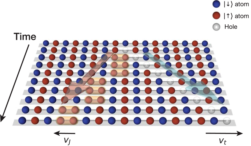
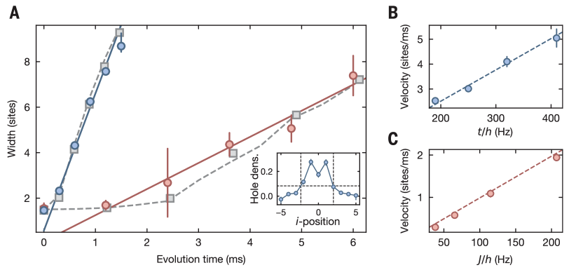
Very recently, the separation of a holon from the two-neighbour spin defect caused by a local quench dynamics of removing a single particle from an initial Mott state in 1D Hubbard model was studied in Ref. Vijayan:2020 . A single atom was simultaneously removed from each chain by using an elliptically shaped near-resonant laser. After such a quench, an obvious difference in the dynamics of spin and charge degrees of freedom was monitored. Consequently, the speed difference between the single hole and the spin configuration defect caused by a quench dynamics was verified, see Fig. 13. The dynamical spin-charge separation in the upper panel of Fig. 13 was interpreted by a quantum walk of single hole in charge sector and the subsequent evolution of spin configuration induced by the local quench in the center of the 1D lattices. Such dynamical evolutions of independent excitations in charge (holon) and spin (spinon) appear to give two independent propagating velocities, see the lower panel of the Fig. 13. The dynamics of holons is read off from the specially resolved hole density distribution in each Hubbard chain, here labels the lattice sizes. Whereas, the dynamics of spinons was measured by the nearest-neighbour spin correlation
| (81) |
in the squeezed space, see Figure 2 in Vijayan:2020 . For a strong interaction, it can be captured by the dynamics of an antiferromagnetic Heisenberg chain. The spin velocity is proportional to the effective spin exchange coupling constant .
The speed difference in the propagation of the single hole and the spinons induced by their quench dynamics provided an evidence for the spin-charge separation phenomenon. However, it does not mean a confirmation of the spin-charge separation phenomenon described by the Luttinger theory. The spin-charge separation theory significantly involves collective motion of bosons in charge and spin degrees of freedom, i.e. the elementary low energy excitations of the system dissolve into two Luttinger liquids which solely carry either spin or charge. Scientifically speaking, a conclusive observation of the spin-charge separation predicted by the Luttinger liquid theory requires: 1) identification of the fractional collective excitation spectra of charge and spin; 2) confirmation of the Luttinger liquid theory in terms of spin and charge correlation functions; 3) determination of spin and charge sound velocities and their Luttinger parameters.
Towards this goal, a recent theoretical study of the Yang-Gaudin model (10) discussed the microscopic origin of the spin-charge separation and gave a proposal for experimental measurement of this phenomenon He:2020 . Following this theoretical scheme, R. Hulet group from Rice University with his theoretical collaborators has observed the independent spin and charge density waves in this model with tunable repulsive interaction Senaratne:2021 . In this experiment, the spin and charge density waves which were encoded by their dynamical correlation functions not only confirm the nature of the Luttinger liquids of spin and charge, but also the nonlinear effects due to the band curvature in charge excitation and backward scattering spin excitation.
Before introducing a new experimental observation of spin-charge separation in the Yang-Gaudin model Senaratne:2021 , here we first recall several concepts of the TLL theory which is used to describe the low energy physics of the Yang-Gaudin model. Following the notation in the book Giamarchi-book , the effective Hamiltonian for the linear charge and spin excitations reads
| (82) |
where and represent the two independent bosonic fields. In the above equations, the fields and its canonically conjugate momentum obeys the standard Bose communication relations , i.e. with . The stands for the variation of a bosonic field . This effective Hamiltonian characterizes the long distance asymptotic decay of correlation function for the 1D Fermi gas. The coefficients for different processes are given phenomenologically in Giamarchi-book . The susceptibilities of charge and spin are defined by
| (83) | |||
| (84) |
where the charge density and spin density are defined by
From the bosonization approach, if , the two dynamic response functions can be obtained by only considering the contributions of the variations and in charge and spin densities, namely
| (85) | |||||
| (86) |
Here are the Luttinger parameter for charge and spin, respectively.
However, the interplay between the spin and charge degrees of freedom leads to subtle difference in effects of band curvatures in these fractionalized spin and charge excitations. Such nonlinearity dispersions in spin and charge degrees of freedom require the newly developed nonlinear TLL theory Imambekov:2009 ; Imambekov:2012 . Whereas for charge sector in the low temperature regime, i.e., and , the broadening of the charge DSF associated the dispersion curvature terms can be well approximated by the imaginary part of the density-density correlation function for free fermions Pereira:2010 ; Cherny:2006 . The charge DSF of 1D noninteracting homogeneous Fermi gas is given by Cherny:2006
| (87) |
where is the dynamic polarizability, its imaginary part can be written by
| (88) |
with
| (89) |
Here is the effective mass of the interacting fermions He:2020 .
In the paper Pereira:2010 , R G Pereira and E Sela derived the nonlinear effects in term of the spin-charge coupling. It turns out that the backward scattering term in spin sector is the next leading order contribution to the low energy excitations. The parameter is a short-distance cutoff. The effective Hamiltonian for the spin excitation in low energy limit can be given by
| (90) | |||||
The spin DSF, at zero temperature, is a -function peak at . However, at low temperatures, one does not have a similar approximation of the DSF in term of noninteracting spinless fermions. Nevertheless, by considering the interaction, the propagator of the dressed spin bosons is given by Pereira:2010
| (91) |
here is the self-energy of spin bosons. It is straightforward to obtain the spin DSF
| (92) |
We assumed that the real part of the retarded self-energy is zero, whereas is given in term of the imaginary part of
| (93) |
where the renormalization coupling constant can be determined by Vijayan:2020
| (94) |
with and g=, here is the interaction strength of the model.
Using Bragg beams to excite charge and spin excitations with the momentum transfer to the system from the Bragg beams is given by
| (95) |
where is the relative detuning of the Bragg beam with respect to each spin state. For charge excitation in experimental setting with , here is the splitting energy between the two spin states, then the momentum transfer for the change density wave. Whereas for spin excitations, , then the momentum transfer . In the above equations, the charge- and spin-density DSF are given by
| (96) |
The two independent DSFs and can be calculated from the dynamic polarizability discussed above. At finite temperatures, the momentum transfer is modified accordingly as , see Senaratne:2021 .
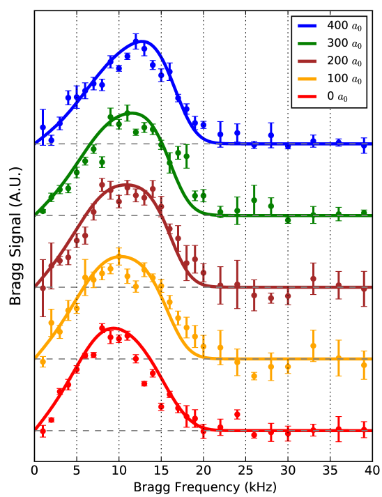
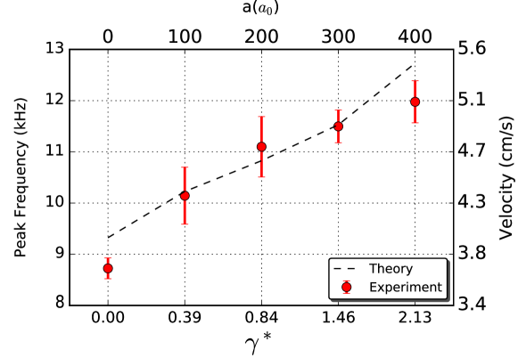
The excitation spectrum of the charge density wave of the Yang-Gaudin model (10) was experimentally observed for various interaction strengths by R. Hulet group at Rice university YangTL:2018 . In this paper they directly measured the charge DSF for a fixed momentum in the ensemble of 6Li atoms in the two energetically hyperfine sublevels and (), see Fig 14. They were for first time to demonstrate experimentally that the charge excitation in the 1D interacting fermions can be approximately described by the DSF of free fermions (87). The agreement between the Bragg signal and theoretical simulation can be seen in Fig 14. They further showed that the velocities read off from the Bragg peak frequency agreed with the results obtained from Bethe ansatz Guan:2013 . The significance of this observation is the manifestation of the Luttinger liquid nature in the collective charge excitation.
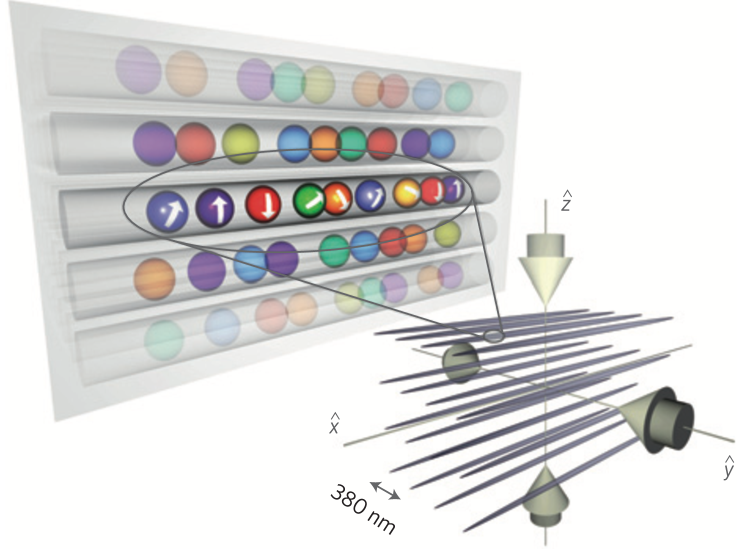
In contrast to the Bragg spectroscopy for the charge excitation, the measurements of the spin Bragg spectra requires that the Bragg photons must be much closer detuned from resonance with the chosen excited state than for the charge-mode measurement. In the recent experiment Senaratne:2021 , a spin-balanced mixture of 6Li atoms was realized in an anisotropic optical trap. In this work, by applying a pair of Bragg beams on the sample in a 200 s pulse, the spin and charge DSFs were independently measured for the quasi-1D trapped Yang-Gaudin Fermi gases, see Fig. 15. By using the pseudo-spin- states and , the detuning from the excited state was reduced by about a factor of two, and the rate of spontaneous emission is correspondingly reduced. More significantly, however, the rate of spontaneous emission was reduced further by using the narrow (UV) transition for the Bragg spectroscopy, rather than the usual (red) transition. Thus the decay linewidth of the state is approximately times narrower than the state Duarte:2011 ; Cherny:2006 , resulting in a total reduction of spontaneous emission for a given Bragg signal by a factor of , in comparison to the previous experiment YangTL:2018 .
To measure the spin Bragg spectra, they chose the states and as the pseudo-spin- states in order to decrease the detuning of the Bragg beams from resonance to reduce the spontaneous emission rate.
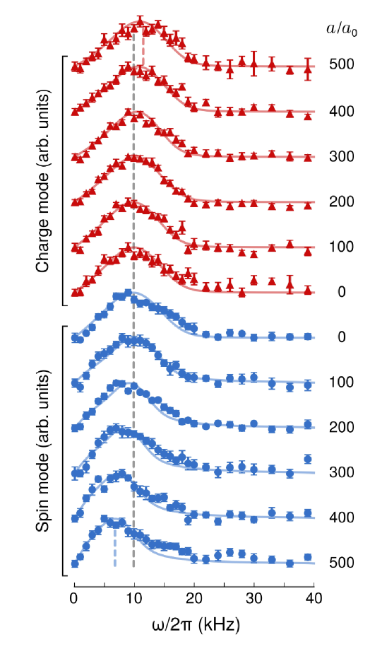
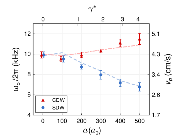
The Fig. 15 shows the measured (symbols) and calculated (solid lines) Bragg spectra for both spin and charge modes in the range of the interactions with the 3D scattering length from 0 to 500 , here is the Bohr radius. The Bragg signal was compared with the calculated charge and spin spectra by invoking the local density approximation, showing excellent agreement between experimental data and theoretical simulations of the charge and spin DSFs from the Eqs. (88) and (92). This agreement significantly confirms the linear Luttinger liquid dynamical correlations with the nonlinear contributions from the curvature effect in charge degree of freedom and backward scattering effect in spin degree of freedom. Moreover, the frequency at which the Bragg signal reaches a maximum, , corresponds to the values of the sound velocities of charge and spin via , in the ensemble of 1D tubes. The lower panel of the Fig. 15 shows agreement between the velocities extracted from the peak frequencies (symbols) and theoretical ones (dashed lines) obtained from the Bethe ansatz solution. The hallmark of the 1D many-body physics–spin-charge separation has been elegantly confirmed in this work. A more detailed study of such novel phenomenon, see He:2020 ; Senaratne:2021 , also the pedagogical book Giamarchi-book .
Experimental measurements of phase diagram and pairing of two-component ultracold atoms trapped in an array of 1D tubes were reported in Liao:2010 ; Revelle:2016 . The trapped fermionic atomic gas was demonstrated a spin population imbalance caused by a difference in the numbers of spin-up and spin-down atoms. Such a novel phase diagram was further investigated by the 1D to 3D crossover of the Yang-Gaudin model with tunable interaction strengths Revelle:2016 .
IV.8 IV.8. Multicomponent Interacting Fermions With Tunable Spin
Fermionic alkaline-earth atoms exhibit an exact spin symmetry Cazalilla:2009 ; Gorshkov:2010 . This discovery has led to rich experimental developments Taie:2010 ; XZhang2014S ; Cappellini2014PRL ; Scazza2014NP , including Kondo spin-exchange physics Nakagawa:2015 ; Zhang2015 , fermionic Hubbard model Ozawa:2018 ; Taie:2020 and Tomonaga-Luttinger liquid (TLL) Pagano:2014 etc. Such multicomponent interacting fermions provide an ideal platform to simulate unusual symmetries in nature. The interplay between the symmetries and interaction leads to striking features of quantum dynamics, thermodynamics as well as magnetocaloric-like effects see recent new developments Taie:2012 ; Hofrichter:2016 ; Goban:2018 ; Song:2020 . The ultracold alkaline-earth atomic gases also provide promising applications in quantum precision measurements.
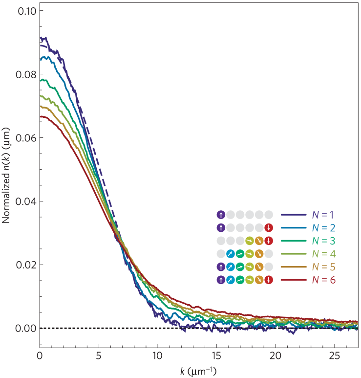
In term of quantum integrability, non-diffraction in the many-particle scattering process displays subtle fractional spin, charge excitations and criticality in the integrable models of interacting fermions with higher symmetries, see review Guan:2013 . In this scenario, the charge excitation mode of fermionic atoms confined to quasi-1D tubes has been previously measured for the 1D Fermi gas with a fixed interaction Pagano:2014 . In this experiment, the authors realized an ensemble of 1D wires of repulsive Fermi gases of 173Yb ultracold atoms with tunable degree from to . The pure nuclear spin results in spin independent interaction such that the system has up to symmetry, see the upper panel in Fig. 16. The authors in Pagano:2014 demonstrated the role of the spin degrees of freedom by measuring the momentum distribution for to . They observed that the broadening of the momentum distribution with a reduction of the weight at low momentum and slower decay at the large momentum tails when the number of spin components increases, see the lower panel in Fig. 16. To understand this feature, we see that the ground state energies for the 1D Fermi gases with weak and strong repulsions Guan:2012b
| (97) | |||||
| (98) |
have less Fermi kinetic energy when the spin degrees increase. In the above equation and . Here and are the Riemann functions, denotes the Euler function, denotes the Euler constant. Therefore, the Fermi gas with larger internal degrees of freedom has less Fermi pressure. Consequently, the trapped Fermi gases in the same axial trapping potential would be more spreading in momentum distribution with increasing the component .
In work Pagano:2014 , by measuring the square ratio of the breathing frequency to the trapped axial frequency , i.e. , the authors further demonstrated an important feature that the ground state energy of the 1D multi-component Fermi gases reduces to the one of the spinless Bose gas. The ratio square reflects this feature of the ground state energy, see Liu:2014 . Their experimental observation can be understood by the calculation of the parameter via the ground state energy of the model. The ground state energy given by (97) and (98) reduce to the one of the Lieb-Liniger gas when we take . For a strong repulsion and in this limit , it was observed Jiang:2015 that the spin velocity vanishes while the charge velocity turns to the one for the Lieb-Liniger Bose gas, namely,
| (99) |
Here . This clearly shows a strong suppression of the Fermi exclusion statistics by the commutativity feature among the -component fermions with different spin states, which was for the first time found by Yang and You in Yang-You:2011 and confirmed by Guan et al. Guan:2012b . This feature was recently confirmed in higher dimensional ultracold atoms Song:2020 . Although they also measured the charge excitation spectrum for different spin states by Bragg spectroscopy tuning, observation of the charge and spin velocities as well as the spin-charge separation in the 1D multicomponent Fermi gases still remains challenging.
In addition, the antiferromagnetic correlations in the 1D, 2D and 3D Hubbard models were studied in Taie:2020 ; Hart:2015 ; Singha:2011 ; Schneider:2012 ; Cheuk:2016 ; Parsons:2016 ; Fujita:2017 . Extending the symmetry in the Mott insulators of the Hubbard model to such higher symmetries could lead to richer magnetic ordering and magnetism than that of the usual electronic correlated systems. The 1D spinor bosonic Hubbard models have provided novel realizations of spin wave quasiparticles (magnons) Fukuhara:2013a ; Fukuhara:2013b , and antiferromagnetic correlations Sun:2021 . Nevertheless, the multicomponent Fermi and Bose gases with tunable mathematical symmetries open to investigate fundamental many-body spin dynamics and magnetism for future quantum technology, for example, fractional heavy spinons and magnons in the 1D Fermi and Bose gases have not observed in experiment.
The study of quantum physics of 1D integrable models are rapidly developing. Recent developments of quantum solvable models comprise new frontiers in various fields such as atomic physics, condensed matter physics, solid state materials and high energy physics, etc. Yang-Baxter integrability also lays out new trends in quantum information, quantum metrology and quantum technology, ranging from quantum heat engine Mukherjee:2021 ; Brantut:2013 ; Hofer:2017 ; Jaramillo:2016 ; Gluza:2021 ; ChenYY:2021 and quantum refrigeration Medley:2011 ; Weld:2010 ; Yu:2020 to quantum battery Strambini:2020 ; Caliga:2017 , atomtronics Amico:2021 , precision measurement Bentsen:2019 ; Cai:2021 ; Grun:2022 ; Kitagawa:2010 , quantum transport Bertini:2021 , quantum control Wilsmann:2018 and quantum impurities Mathy:2012 ; Meinert:2017 ; Knap:2014 ; Dolgirev:2021 ; Dehkharghani:2018 . In this short review, our aim was not to review all such developments. Instead we briefly discussed some highlights: several Yang-Baxter solvable models, including the Lieb-Liniger model Lieb-Liniger:1963 , the Yang-Gaudin model Yang:1967 ; Gaudin:1967 , the Fermi gases Sutherland:1968 , the GHD theory, the Haldane’s FES and compared them with recent novel experiments. In particular, the newly developed theory of GHD Castro:2016 ; Bertini:2016 coming along with experimental observations of the quantum Newtons’s cradle and the corresponding description in terms of GHD has been discussed in details. Several other important experiments on dynamical fermionization, quantum criticality, Luttinger liquid, the Haldane’s fractional exclusion statistics, quantum holonomy, spin-charge separation and quantum impurity have been discussed and highlighted. It turns out that integrable models of ultracold atoms provide an ideal platform to experimentally study quantum dynamics, hydrodynamics and thermodynamics at a many-body level. Here an outlook is made for future research on the Yang-Baxter integrability with ultracold atoms:
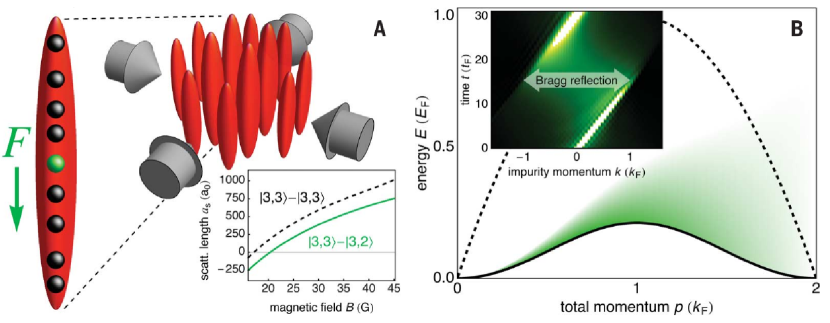
(a) Sensoring gravitational force: In a recent paper Meinert:2017 , the Bloch oscillation of an impurity atom was found in the continuum liquid of 1D interacting Bose gas, see Fig. 17 (A). Adding an impurity atom with the same mass into a degenerate 1D gas of Cesium atoms trapped in each tube of the 3D ensemble, F. Meinert et al. observed Bloch oscillation in the dynamics of the impurity atom of hyperfine state , on which a (dimensionless) gravitation force acts, here was the density of the host atoms and denoted the gravitational force. It was remarkable to find that the characteristic Bragg reflection occurred in the absence of a lattice, which was considered the key setting for the usual Bloch oscillations caused by periodic momentum dependent eigenstates. That was mainly because the magnon excitation had a collective cosine-shaped dispersion which resembled the conventional dispersion of magnon in a 1D lattice, see Fig. 17 (B). The periodicity was 2, where the Fermi momentum . This gave an effective Brillouin zone. The impurity atom thus exhibited Bragg reflection at the edge of this Brillouin zone. The excess momentum dissolved into particle-hole excitations of the host atoms of the state . Although the observed Bloch oscillations in such interacting 1D Bose gas were not perfect due to the strong many-body correlation effects, the experiment holds a promise for future quantum technology in sensoring weak force.
Nevertheless, nonequilibrium dynamics of Newtons’s cradle Kinoshita:2006 , hydrodynamics of quasi-1D trapped gases in a double-well potential Schemmer:2019 , quantum walks and Bloch oscillations of bosons and fermions in a 1D lattice Preiss:2015 will lead to potential applications in high precision measurement of the gravitational force and testing the Einstein equivalence principle. These settings will highlight the importance of quantum coherence and entanglement in quantum many-body dynamics out-of-equilibrium, in particular in systems with higher mathematical symmetries. Studying quantum transport and conductivity of 1D many-body systems in the frame work of the GHD and Bethe ansatz still remain an open challenge.
(b) Quantum many-body entanglement: The observation of spin-charge separation phenomenon Vijayan:2020 ; Senaratne:2021 open the possibility to further study novel spin states and fractional quasiparticles in 1D ultracold atoms. The experiment Senaratne:2021 remarkably provides a conclusive observation of the spin-charge separation in Luttinger liquids and also goes beyond it. Further studies of spin coherent and incoherent Luttinger liquids in the 1D Hubbard model, quantum gases with and fermionic atoms with higher spin symmetries etc. is highly desirable. On the other hand, it was recently shown Hauke:2016 that the dynamical response function of spinons can be used to measure multipartite entanglement in quantum spin systems. The key to this study relies on the connection between the quantum Fisher information and dynamic susceptibility. The former can be used as a witness of the multipartite entanglement in quantum many-body systems. This was experimentally demonstrated Scheie:2021 ; Laurell:2022 ; Zhang:2014 that the neutron scattering DSF can witness the entanglement of spins in the 1D Heisenberg chain. This opens promising opportunities to explore realistic applications of fractional excitations, spin liquids and impurities in quantum metrology. Moreover, quantum entanglement in 1D topological matter Leseleuc:2019 ; Kanungo:2022 ; Atala:2022 and integrable models with Lindblad dissipations Ziolkowska:2020 ; Bacsi:2020 ; Nakagawa:2021 ; Landi:2022 ; Popkov:2022 ; Rosso:2022 comprise new frontiers in quantum integrability.
(c) Quantum heat engine and refrigeration: Many-body physics presents fundamental principles which will play a key role in future quantum technologies. The study of quantum cooling and heat engine Mukherjee:2021 ; Brantut:2013 ; Hofer:2017 ; Jaramillo:2016 ; Gluza:2021 ; ChenYY:2021 in ultracold atomic physics still remains rather elusive. To achieve the goal of cooling interacting fermions, it requires us to understand caloric effects induced by magnetic field, trapping potential and dynamical interaction as well as adiabatic evolutions of the energy and currents during strokes Medley:2011 ; Weld:2010 ; Yu:2020 ; Daniloff:2021 . For those research, one has many open questions regarding the quantum speed of adiabatic processes and heat exchanges between the system and baths and caloric effects. The interaction ramp up and down near a quantum phase transition in quantum gases provide a promising protocol of quantum refrigeration besides the usual adiabatic demagnetization cooling in solid-state materials Wolf:2011 . Exactly solvable models of quantum gases, strongly correlated electrons and spins thus exhibit rich phases of quantum matter which will provide important benchmarks and quantum advantage for studying quantum heat engine, quantum refrigeration and quantum batteries in quantum technology. And more generally, mathematical models provide an ideal platform to advance our understanding of new quantum effects for future technology, including quantum metrology, quantum information and quantum communication.
Acknowledgements.
X.W.G. is supported by the NSFC key grant No. 12134015, the NSFC grant No. 11874393 and No. 12121004. The authors thank Angela Foerster, H Pu, Hui Hu, Xia-Ji Liu, Zhen-Sheng Yuan, Shi-Guo Peng, Sheng Wang for helpful discussions. They thank Randy Hulet and Natan Andrei for their help with going through the manuscript.References
- (1) Bethe H 1931 Z. Phys. 71 205
- (2) Lieb E H and Liniger W 1963 Phys. Rev. 130 1605
- (3) Yang C N 1967 Phys. Rev. Lett. 19 1312
- (4) Gaudin M 1967 Phys. Lett. A 24 55
- (5) Lieb E H and Wu F Y 1968 Phys. Rev. Lett. 20 1445
- (6) Sutherland B 1968 Phys. Rev. Lett. 20 98
- (7) Andrei N 1980 Phys. Rev. Lett. 45 98
- (8) Wiegmann P B 1980 Phys. Rev. Lett. 80 163
- (9) Tsvelik A and Wiegmann P 1983 Adv. Phys. 32 453
- (10) Andrei N, Furuya K and Lowenstein J H 1983 Rev. Mod. Phys. 55 331
- (11) Bardeen J, Cooper L N and Schrieffer J R 1957 Phys. Rev. 108 1175
- (12) Richardson R W 1963 Phys. Lett. 3 277; Phys. Lett. 5 82
- (13) Dukelsky J, Pittel S and Sierra G 2004 Rev. Mod. Phys. 76 643
- (14) Cazalilla M A, Citro R, Giamarchi T, Orignac E and Rigol M 2011 Rev. Mod. Phys. 83 1405
- (15) Guan X W, Batchelor M T and Lee C 2013 Rev. Mod. Phys. 85 1633
- (16) Batchelor M T and Foerster A 2016 J. Phys. A: Math. Theor. 49 173001
- (17) Mistakidis S I, Volosniev A G, Barfknecht R E, Fogarty T, Busch T, Foerster A, Schmelcher P and Zinner N T 2022 arXiv:2202.11071
- (18) Giorgini S, Pitaevskii L P and Stringari S 2008 Rev. Mod. Phys. 80 1215
- (19) Lewenstein M, Sanpera Anna, Ahufinger V, Damski B, Sen(De) A and Sen U 2007 Adv. Phys. 56 243
- (20) Kinoshita T, Wenger T and Weiss D S 2004 Science 305 1125
- (21) Paredes B, Widera A, Murg V, Mandel O, Föling S, Cirac I, Shlyapnikov G V, Hänsch T W and Bloch I 2004 Nature (London) 429 277
- (22) Kinoshita T, Wenger T and Weiss D S 2005 Phys. Rev. Lett. 95 190406
- (23) van Amerongen A H, van Es J J P, Wicke P, Kheruntsyan K V and van Druten N J 2008 Phys. Rev. Lett. 100 090402
- (24) Armijo J, Jacqmin T, Kheruntsyan K V and Bouchoule I 2010 Phys. Rev. Lett. 105 230402
- (25) Jacqmin T, Armijo J, Berrada T, Kheruntsyan K V and Bouchoule I 2011 Phys. Rev. Lett. 106 230405
- (26) Stimming H P, Mauser N J, Schmiedmayer J and Mazets I E 2010 Phys. Rev. Lett. 105 015301
- (27) Armijo J 2012 Phys. Rev. Lett. 108 225306
- (28) Vogler A, Labouvie R, Stubenrauch F, Barontini G, Guarrera V and Herwig Ott 2013 Phys. Rev. A 88 031603(R)
- (29) Astrakharchik G E, Boronat J, Casulleras J and Giorgini S 2005 Phys. Rev. Lett. 95 190407
- (30) Batchelor M T, Bortz M, Guan X W and Oelkers N 2005 J. Stat. Mech. 10 L10001
- (31) Haller E, Gustavsson M, Mark M J, Danzl J G, Hart R, Pupillo Guido and Nägerl H C 2009 Science 325 1224
- (32) Kao W, Li K Y, Lin K Y, Gopalakrishnan S and Lev B L 2021 Science 371 296
- (33) Moritz H, Stöferle T, Günter K, Köhl M and Esslinger T 2005 Phys. Rev. Lett. 94 210401
- (34) Liao Y, Rittner A S C, Paprotta T, Li W, Partridge G B, Hulet R G, Baur S K and Mueller E J 2010 Nature 467 567
- (35) Zürn G, Serwane F, Lompe T, Wenz A N, Ries M G, Bohn J E and Jochim S 2012 Phys. Rev. Lett. 108 075303
- (36) Zürn G, Lompe T, Wenz A N, Jochim S, Julienne P S and Hutson J M 2013 Phys. Rev. Lett. 110 135301
- (37) Zürn G, Wenz A N, Murmann S, Bergschneider A, Lompe T and Jochim S 2013 Phys. Rev. Lett. 111 175302
- (38) Wenz A N, Zürn G, Murmann S, Brouzos I, Lompe T and Jochim S 2013 Science 342 6157
- (39) Murmann S, Deuretzbacher F, Zürn G, Bjerlin J, Reimann S M, Santos L, Lompe T and Jochim S 2015 Phys. Rev. Lett. 115 215301
- (40) Revelle M C, Fry J A, Olsen B A and Hulet R G 2016 Phys. Rev. Lett. 117 235301
- (41) Pagano G et al 2014 Nat. Phys. 10 198
- (42) Song B, Yan Y, He C, Ren Z, Zhou Q, and Jo G B 2020 Phys. Rev. X 10 041053
- (43) Wu C, Hu J P, and Zhang S C 2003 Phys. Rev. Lett. 91 186402
- (44) Wu C 2006 Mod. Phys. Lett. B 20 1707
- (45) Yang T L, Grišins P, Chang Y T, Zhao Z H, Shih C Y, Giamarchi T and Hulet R G 2018 Phys. Rev. Lett. 121 103001
- (46) Haller E et al 2010 Nature 466 597
- (47) Fabbri N, Panfil M, Clément D, Fallani L, Inguscio M, Fort C and Caux J S 2015 Phys. Rev. A 91 043617
- (48) Meinert F, Panfil M, Mark M J, Lauber K, Caux J S and Nägerl H C 2015 Phys. Rev. Lett. 115 085301
- (49) Yang B, Chen Y Y, Zheng Y G, Sun H, Dai H N, Guan X W, Yuan Z S and Pan J W 2017 Phys. Rev. Lett. 119 165701
- (50) Schweigler T et al 2017 Nature 545 323
- (51) Prüfer M, Kunkel P, Strobel H, Lannig S, Linnemann D, Schmied C M, Berges J, Gasenzer T and Oberthaler M K 2018 Nature 563 217
- (52) Wilson J M, Malvania N, Le Y, Zhang Y, Rigol M and Weiss D S 2020 Science 367 1461
- (53) Tang Y, Kao W, Li K Y, Seo S, Mallayya K, Rigol M, Gopalakrishnan S and Lev B L 2018 Phys. Rev X 8 021030
- (54) Erne S, Büker R, Gasenzer T, Berges J, and Schmiedmayer J 2018 Nature 563 225
- (55) Sun H, Yang B, Wang H Y, Zhou Z Y, Su G X, Dai H N, Yuan Z S and Pan J W 2021 Nat. Phys. 17 990
- (56) Boll M, Hilker T A, Salomon G, Omran A, Nespolo J, Pollet L, Bloch I and Gross C 2016 Science 353 1257
- (57) Hilker T A, Salomon G, Grusdt F, Omran A, Boll M, Demler E, Bloch I and Gross C 2017 Science 357 484
- (58) Vijayan J et al 2020 Science 367 186
- (59) Spar B M, Guardado-Sanchez E, Chi S, Yan Z Z and Bakr W S 2022 Phys. Rev. Lett. 128, 223202
- (60) Chang Y T, Senaratne R, Cavazos-Cavazos D and Hulet R 2020 Phys. Rev. Lett. 125 263402
- (61) Ahmed-Braun D J M, Jackson K G, Smale S, Dale C J, Olsen B A, Kokkelmans S J J M F, Julienne P S and Thywissen J H Phys. Rev. Research 3 033269
- (62) Jackson K G et al 2022 arXiv:2206.10415
- (63) Venu V et al 2022 arXiv:2205.13506
- (64) Yurovsk V A, Malomed B A, Hulet R G and Olshanii M 2017 Phys. Rev. Lett. 119 220401
- (65) Luo D et al 2020 Phys. Rev. Lett. 125 183902
- (66) Marchukov O V et al 2020 Phys. Rev. Lett. 125 050405
- (67) Vidmar L et al 2015 Phys. Rev. Lett. 115, 175301
- (68) Kinoshita T, Wenger T and Weiss D S 2006 Nature 440 900
- (69) Rigol M, Dunjko V, Yurovsky V and Olshanii M 2007 Phys. Rev. Lett. 98 050405
- (70) Ilievski E, De Nardis J, Wouters B, Caux J S, Essler F H and Prosen T 2015 Phys. Rev. Lett. 115 157201
- (71) Castro-Alvaredo O A, Doyon B and Yoshimura T 2016 Phys. Rev. X 6 041065
- (72) Bertini B, Collura M, De Nardis J and Fagotti M 2016 Phys. Rev. Lett. 117 207201
- (73) Langen T et al 2015 Science 348 207
- (74) Schemmer M, Bouchoule I, Doyon B and Dubail J 2019 Phys. Rev. Lett. 122 090601
- (75) Malvania N, Zhang Y, Le Y, Dubail J, Rigol M and Weiss D S 2021 Science 373 1129
- (76) Moller F et al 2021 Phys. Rev. Lett. 126 090602
- (77) Li C et al 2020 SciPost Phys. 9 058
- (78) Cataldini F et al 2021 arXiv: 2111.13647v2
- (79) van den Berg R, Wouters B, Eliëns S, De Nardis J, Konik R M and Caux J S 2016 Phys. Rev. Lett. 116 225302
- (80) Caux J S, Doyon B, Dubail J, Konik R and Yoshimura T 2019 SciPost Phys. 6 070
- (81) De Nardis J, Bernard D and Doyon B 2018 Phys. Rev. Lett. 121 160603
- (82) Bastiannello A, Alba V and Cau J S 2019 Phys. Rev. Lett. 123 130602
- (83) Bastiannello A, De Luca A, Doyon B and De Nardis J 2020 Phys. Rev. Lett. 125 240604
- (84) Ruggierro P, Calabrese P, Doyon B and Dubail J 2020 Phys. Rev. Lett. 124 140603
- (85) Doyon B, Dubail J, Konik R and Yoshimura T 2017 Phys. Rev. Lett. 119 195301
- (86) Fava M, Biswas S, Gopalakrishnan S, Vasseur R and Parameswaran S A 2021 Proc. Nat. Acad. Sci. USA 118 e2106945118
- (87) Bastianello A, Bertini B, Doyon B and Vasseur R 2022 J. Stat. Mech 014001
- (88) Bouchoule I and Dubail J 2022 J. Stat. Mech. 014003
- (89) Moller F, Erne S, Mauser N J , Schmiedmayer J and Mazets I E 2022 arXiv:2205.15871
- (90) Bertinit B, Essler F H L and Granet E 2022 Phys. Rev. Lett. 128 190401
- (91) Fukuhara T et al 2013 Nat. Phys. 9 235
- (92) Fukuhara T, Schauß P, Endres M, Hild S, Cheneau M, Bloch I and Gross C 2013 Nature 502 76
- (93) Catani J, Lamporesi G, Naik D, Gring M, Inguscio M, Minardi F, Kantian A and Giamarchi T 2012 Phys. Rev. A 85 023623
- (94) Meinert F, Knap M, Kirilov E, Jag-Lauber K, Zvonarev M B, Demler E and Nägerl H C 2017 Science 356 945
-
(95)
Zhang X B, Chen Y Y, Liu L X, Deng Y J and Guan X W 2022 Natl. Sci. Rev.,
https://doi.org/10.1093/nsr/nwac027 - (96) Senaratne R, Cavazos-Cavazos D, Wang S, He F, Chang Y T, Kafle A, Pu H, Guan X W and Hulet R G 2022 Science 376, 1305
- (97) Olshanii M 1998 Phys. Rev. Lett. 81 938
- (98) Dunjko V, Lorent V, and Olshanii M 2001 Phys. Rev. Lett. 86 5413
- (99) Olshanii M and Dunjko V 2003 Phys. Rev. Lett. 91 090401
- (100) Jiang Y Z, Chen Y Y and Guan X W 2015 Chin. Phys. B 24 050311
- (101) Yang C N and Yang C P 1969 J. Math. Phys. 10 1115
- (102) Guan X W and Batchelor M T 2011 Journal Physics A: Math. Theor. 44 102001
-
(103)
Baxter R J 1972 Ann. Phys. (N. Y.) 70 193;
Baxter R J 1972 Ann. Phys. (N. Y.) 70 323 - (104) Zhang C, Li J L, Song S Y and Long G L 2013 J. Opt. Soc. Am. B 30 1688
- (105) Vind F A, Foerster A, Oliveira I S, Sarthour R S, Soares-Pinto D O, Souza A M and Roditi I 2016 Sci. Rep. 6 20789
- (106) Essler F H L, Frahm H, Göhmann F, Klümper A and Korepin V E 2005 The One-Dimensional Hubbard Model (Cambridge: Cambridge University Press)
- (107) Korepin V E, Izergin A G and Bogoliubov N M 1993 Quantum Inverse Scattering Method and Correlation Functions (Cambridge: Cambridge University Press)
- (108) Sutherland B 2004 Beautiful Models: 70 years of exactly solved quantum many-body problems (Singapore: World Scientific)
- (109) Takahashi M 1999 Thermodynamics of One-Dimensional Solvable Models (Cambridge: Cambridge University Press)
- (110) Wang Y P, Yang W L, Cao J P and Shi K J 2015 Off-Diagonal Bethe Ansatz for Exactly Solvable Models (Berlin: Springer-Verlag Berlin Heidelberg)
- (111) Scopa S, Calabrese P and Piroli L 2021 Phys. Rev. B 104 115423
- (112) Girardeau M 1960 J. Math. Phys. 1 516
- (113) Girardeau M 1965 Phys. Rev. 139 B500
- (114) Minguzzi A and Gangardt D M 2005 Phys. Rev. Lett. 94 240404
- (115) Rigol M and Muramatsu A 2005 Phys. Rev. Lett. 94 240403
- (116) Lyer D and Andrei N 2012 Phys. Rev. Lett. 109 115304
- (117) Buljan H, Pezer R and Gasenzer T 2008 Phys. Rev. Lett. 100 080406
- (118) Bolech C J, Heidrich-Meisner F, Langer S, McCulloch I P, Orso G and Rigol M 2012 Phys. Rev. Lett. 109 110602
- (119) Campbell A S, Gangardt D M and Kheruntsyan K V 2015 Phys. Rev. Lett. 114 125302
- (120) Xu W and Rigol M 2017 Phys. Rev. A 95 033617
- (121) del Campo A 2008 Phys. Rev. A 78 045602
- (122) Alam S S, Skaras T, Yang L and Pu H 2021 Phys. Rev. Lett. 127 023002
- (123) Patu O I 2022 Phys. Rev. A 105 063309
- (124) Piroli L and Calabrese P 2017 Phys. Rev. A 96, 023611
- (125) Chen S, Guan X W, Yin X, Guan L and Batchelor M T 2010 Phys. Rev A 81 031608
- (126) Chen S, Guan L, Yin X, Hao Y and Guan X W 2010 Phys. Rev A 81 031609(R)
- (127) Yonezawa N, Tanaka A and Cheon T 2013 Phys. Rev. A 87 062113
- (128) Panfil M and Caux J S 2014 Phys. Rev. A 89 033605
- (129) Kormos M, Mussardo G and Trombettoni A 2011 Phys. Rev. A 83 013617
- (130) Girardeau M D and Astrakharchik G E 2009 Phys. Rev. A 81 061601(R)
- (131) Yin X, Guan X W, Batchelor M T and Chen S 2011 Phys. Rev. A 83 013602
- (132) Imambekov A, Lukyanov A A, Glazman L I and Gritsev V 2010 Phys. Rev. Lett. 104 040402
- (133) Lai C K, 1971 Phys. Rev. Lett. 26 1472
- (134) Lai C K, 1973 Phys. Rev. A 8 2567
-
(135)
Takahashi M 1971 Prog. Theor. Phys. 46 401;
Takahashi M 1971 Prog. Theor. Phys. 46 1388 - (136) Guan X W, Yin X G, Foerster A, Batchelor M T, Lee C H, Lin H Q 2013 Phys. Rev. Lett. 111 130401
- (137) Peng L, Yu Y C and Guan X W 2019 Phys. Rev. B 100 245435
- (138) Yu Y C, Zhang S Z and Guan X W 2020 Phys. Rev. Research 2 043066
- (139) Guan X W, Batchelor M T, Lee C and Bortz M 2007 Phys. Rev. B 76 085120
- (140) Takahashi M 1970 Prog. Theor. Phys. 44 899
- (141) Gu C H and Yang C N 1989 Commun. Math. Phys. 122 105
- (142) Larkin A I and Ovchinnikov Y N 1965 Sov. Phys. JETP 20 762
- (143) Fulde P and Ferrell R A 1964 Phys. Rev. 135 A550
- (144) Yang K 2001 Phys. Rev. B 63 140511(R)
- (145) Orso G 2007 Phys. Rev. Lett. 98 070402
- (146) Hu H, Liu X J and Drummond P D 2007 Phys. Rev. Lett. 98 070403
- (147) Liu X J, Hu H and Drummond P D 2008 Phys. Rev. A 78 023601
- (148) Zhao E, Guan X W, Liu W V, Batchelor M T and Oshikawa M 2009 Phys. Rev. Lett. 103 140404
- (149) Lee J Y and Guan X W 2011 Nucl. Phys. B 853 125
- (150) He J S, Foerster A, Guan X W and Batchelor M T 2009 New J. Phys. 11 073009
- (151) Cazalilla M, Ho A and Ueda M 2009 New J. Phys. 11 103033
- (152) Gorshkov A V, Hermele M, Gurarie V, Xu C, Julienne P S, Ye J, Zoller P, Demler E, Lukin M D and Rey A M 2010 Nat. Phys. 6 289
- (153) Taie S, Takasu Y, Sugawa S, Yamazaki R, Tsujimoto T, Murakami R and Takahashi Y 2010 Phys. Rev. Lett. 105 190401
- (154) Zhang X, Bishof M, Bromley S L, Kraus C V, Safronova M S, Zoller P, Rey A M and Ye J 2014 Science 345 1467
- (155) Cappellini G, Mancini M, Pagano G, Lombardi P, Livi L, de Cumis M S, Cancio P, Pizzocaro M, Calonico D, Levi F, Sias C., Catani J, Inguscio M and Fallani L 2014 Phys. Rev. Lett. 113 120402
- (156) Scazza F, Hofrichter C, Höfer M, Groot P C D, Bloch I and Fölling S 2014 Nat. Phys. 10 779
- (157) Nakagawa M and Kawakami N 2015 Phys. Rev. Lett. 115 165303
- (158) Zhang R, Zhang D, Cheng Y, Chen W, Zhang P and Zhai H 2016 Phys. Rev. A 93 043601
- (159) Batchelor M. T., Guan X.-W., Oelkers N., and Tsuboi Z. 2007 Adv. Phys. 56 465
- (160) Schlottmann P 1997 Int. J. Mod. Phys. B 11 355
- (161) Lee J Y, Guan X W and Batchelor M T 2011 J. Phys. A: Math. Theor. 44 165002
- (162) Guan X W and Ma Z Q 2012 Phys. Rev. A 85 033632
- (163) Guan X W, Ma Z Q and Wilson B 2012 Phys. Rev. A 85 033633
- (164) Jiang Y Z, He P and Guan X W 2016 J. Phys. A: Math. Theor. 49 174005
- (165) Liu X J and Hu H 2014 Ann. Phys. 350 84
-
(166)
Schlottmann P 1993 J. Phys. Condens. Matter 5 5869;
Schlottmann P 1994 J. Phys. Condens. Matter 6 1359 - (167) Yang C N and You Y Z 2011 Chin. Phys. Lett. 28 020503
- (168) Doyon B B and Yoshimura T 2017 SciPost Phys. Lect. Phys. 2 014
- (169) Doyon B 2020 SciPost Phys. Lect. Notes 18, A note on generalized hydrodynamics: inhomogeneous fields and other concepts, https://scipost.org/SciPostPhysLectNotes.18
- (170) Hofferberth S, Lesanovsky I, Fischer B, Schumm T and Schmiedmayer J 2007 Nature 449 324
- (171) Ronzheimer J P 2013 Phys. Rev. Lett. 110 205301
- (172) Haldane F D M 1981 Phys. Rev. Lett. 47 1840
- (173) Giamarchi T 2004 Quantum physics in one dimension (Oxford: Oxford University Press)
- (174) Cazalilla M A 2004 J. Phys. B: At., Mol. Opt. Phys. 37 S1
- (175) Cedergren K, Ackroyd R, Kafanov S, Vogt N, Shnirman A, and Duty T 2017 Phys. Rev. Lett. 119 167701
- (176) Giamarchi T 2017 Physics 10 115
- (177) Khare A 2005 Fractional statistics and quantum theory (Singapore: World Scientific Publishing Co. Pte. Ltd.)
- (178) Leinaas J M, and Myrheim J 1997 Nuovo Cimento B 37 1
-
(179)
Wilczek F 1982 Phys. Rev. Lett. 48 1144;
Wilczek F 1982 Phys. Rev. Lett. 49 957 - (180) Arovas D, Schrieffer J R and Wilczek F 1984 Phys. Rev. Lett. 53 722
-
(181)
Laughlin R B 1988 Phys. Rev. Lett. 60 2677;
Laughlin R B 1988 Science 242 525 - (182) Haldane F D M 1991 Phys. Rev. Lett. 67 937
- (183) Wu Y S Phys. Rev. Lett. 73 922
- (184) Ha Z N C 1994 Phys. Rev. Lett. 73 1574
- (185) Isakov S B 1994 Phys. Rev. Lett. 73 2150
-
(186)
Calogero F 1969 J. Math. Phys. 10 2191;
Calogero F 1969 J. Math. Phys. 10 2197 - (187) Sutherland B J. Math. Phys. 12 251
- (188) Bernard D, and Wu Y S 1995 A note on statistical interactions and the thermodynamic Bethe ansatz, ain Proceedings of the 6th Nankai Workshop, edited by M.L. Ge and Y. S. Wu (Singapore: World Scientific)
- (189) Kundu A 1999 Phys. Rev. Lett. 83 1275
- (190) Batchelor M T, Guan X W and Oelkers N 2006 Phys. Rev. Lett. 96 210402
- (191) He F, Jiang Y Z, Yu Y C, Lin H Q and Guan X W 2017 Phys. Rev. B 96 220401(R)
- (192) Zhang X, Hung C L, Tung S K and Chin C 2012 Science 335 1070
- (193) Hung C L, Zhang X, Gemelke N and Chin C 2011 Nature 470 236
- (194) Batchelor M T and Guan X W 2007 Laser Phys. Lett. 4 77
- (195) Auslaender O M, Yacoby A, de Picciotto R, Baldwin K W, Pfeiffer L N and West K W 2022 Science 295 825
- (196) Auslaender O M, Steinberg H, Yacoby A, Tserkovnyak Y, Halperin B I, Baldwin K W, Pfeiffer L N and West K W 2005 Science 308 88
- (197) Jompol Y, Ford C J B, Griffiths J P, Farrer I, Jones G A C, Anderson D, Ritchie D A, Silk T W and Schofield A J 2009 Science 325 597
- (198) Segovia P, Purdie D, Hengsberger M, Baer Y 1999 Nature 402 504
- (199) Kim C, Matsuura A Y, Shen Z X, Motoyama N, Eisaki H, Uchida S, Tohyama T and Maekawa S 1996 Phys. Rev. Lett. 77 4054
- (200) Kim B J et al 2006 Nat. Phys. 2 397
- (201) He F, Jiang Y Z, Lin H Q, Hulet R G, Pu H and Guan X W 2020 Phys. Rev. Lett. 125 190401
- (202) Imambekov A and Glazman L I 2009 Science 323 228
- (203) Imambekov A, Schmidt T L and Glazman L I 2012 Rev. Mod. Phys. 84 1253
- (204) Pereira R G and Sela E 2010 Phys. Rev. B 82 115324
- (205) Cherny A Y and Brand J 2006 Phys. Rev. A 73 023612
- (206) Mukherjee V and Divakaran U 2021 J. Phys. Condens. Matter 33 454001
- (207) Brantut J P, Grenier C, Meineke J, Stadler D, Krinner S, Kollath C, Esslinger T and Georges A 2013 Science 342 713
- (208) Hofer P P, Brask J B, Perarnau-Llobet M and Brunner N 2017 Phys. Rev. Lett. 119 090603
- (209) Jaramillo J, Beau M and del Campo A 2016 New J. Phys. 18 075019
- (210) Gluza M et al 2021 Phys. Rev. X Quantum 2 030310
- (211) Chen Y Y, Watanabe G, Yu Y C, Guan X W and del Campo A 2019 npj Quantum Inf 5 88
- (212) Medley P, Weld D M, Miyake H, Pritchard D E and Ketterle W 2011 Phys. Rev. Lett. 106 195301
- (213) Weld D M, Miyake H, Medley P, Pritchard D E and Ketterle W 2010 Phys. Rev. A 82 051603
- (214) E. Strambini et al 2020 Nat. Nanotech. 15 565
- (215) Caliga S C, Straatsma C J E and Anderson D Z 2017 New J. Phys. 19 013036
- (216) Mathy C J M, Zvonarev M B and Demler E 2012 Nat. Phys. 8 881
- (217) Knap M, Mathy C J, Ganahl M, Zvonarev M B and Demler E 2014 Phys. Rev. Lett. 112 015302
- (218) Dolgirev P E, Qu Y F, Zvonarev M B, Shi T and Demler E 2021 Phys. Rev. X 11 041015
- (219) Dehkharghani A S, Volosniev A G and Zinner N T 2018, Phys. Rev. Lett. 121, 080405
- (220) Amico L et al 2021 AVS Quantum Sci. 3 039201
- (221) Bentsen G, Potirniche I D, Bulchandani V B, Scaffidi T, Cao X, Qi X L, Schleier-Smith M and Altman E 2019 Phys. Rev. X 9 041011
- (222) Cai X, Yang H, Shi H L, Lee C, Andrei N and Guan X W 2021 Phys. Rev. Lett. 127 100406
- (223) ] Grün D S, Wittmann K, Ymai L, Links J and Foerster A 2022 Commun. Phys. 5 36
- (224) Kitagawa T, Pielawa S, Imambekov A, Schmiedmayer J, Gritsev V and Demler E 2010 Phys. Rev. Lett. 104 255302
- (225) Wilsmann K W, Ymai L H, Tonel A P, Links J and Foerster A 2018 Commun. Phys. 1 91
- (226) Bertini B, Heidrich-Meisner F, Karrasch C, Prosen T, Steinigeweg R and Žnidarič M 2021 Rev. Mod. Phys. 93 025003
- (227) Preiss P M, Ma R, Tai M E, Lukin A, Rispoli M, Zupancic P, Lahini Y, Islam R and Greiner M 2015 Science 347 1229
- (228) Hauke P, Heyl M, Tagliacozzo L and Zoller P 2016 Nat. Phys. 12 778
- (229) Scheie A, Laurell P, Samarakoon A M, Lake B, Nagler S E, Granroth G E, Okamoto S, Alvarez G and Tennant D A 2021 Phys. Rev. B 103 224434
- (230) Laurell P, Scheie A, Tennant A, Okamoto S, Alvarez G and Dagotto E 2022 Phys. Rev. B 106 085110
- (231) Zhang X, Bishof M, Bromley S L, Kraus C V, Safronova M S, Zoller P, Rey A M and Ye J 2014 Science 345 1467
- (232) Léséleuc S de et al 2019 Science 365 775
- (233) Kanungo S K et al 2022 Nat. Commun. 13 972
- (234) Atala M, Aidelsburger M, Barreiro J T, Abanin D, Kitagawa T, Demler E and Bloch I 2013 Nat. Phys. 9 795
- (235) Ziolkowska A A and Essler F H L 2020 SciPost Phys. 8 044
- (236) Bácsi Á, Moca C M, Zaráand G and Dóra B 2020 Phys. Rev. Lett. 125 266803
- (237) Nakagawa M, Kawakami N and Ueda M 2021 Phys. Rev. Lett. 126 110404
- (238) Landi G T, Poletti D and Schaller G 2021 arXiv:2104.14350v3
- (239) Popkov V and Salerno M 2022 arXiv:2206.06771
- (240) Rosso L, Biella A, Nardis J de and Mazza L 2022 arXiv:2206.06837
- (241) Hofrichter C, Riegger L, Scazza F, Höfer Moritz, Fernandes D R, Bloch I and Fölling S 2016 Phys. Rev. X 6 021030
- (242) Goban A 2018 Nature 563 369
- (243) Ozawa H, Taie S, and Takahashi Y 2018 Phys. Rev. Lett. 121 225303
- (244) Taie S, Ibarra-Garc-Padilla E, Nishizawa N, Takasu Y, Kuno Y, Wei H T, Scalettar R T, Hazzard K R A and Takahashi Y 2020 arXiv:2010.07730
- (245) Taie S, Yamazaki R, Sugawa S and Takahashi Y 2012 Nat. Phys. 8 825
- (246) del Daniloff C, Tharrault M, Enesa C and Salomon C 2021 Phys. Rev. Lett. 127 113602
- (247) Wolf B, Tsui Y, Jaiswal-Nagar D, Tutsch U, Honecker A, Remović-Langer K, Hofmann G, Prokofiev A, Assmus W, Donath G and Lang M 2011 Proc. Natl. Acad. Sci. USA 108 6862
- (248) Hart R. A et al 2015 Nature 519 211
- (249) Singha A et al 2011 Science 332 1176
- (250) Schneider U et al 2012 Nat. Phys. 8 213
- (251) Cheuk L. W et al 2016 Science 353 1260
- (252) Parsons M F, Mazurenko A, Chiu C S, Ji G, D. Greif and Greiner M 2016 Science 353 1253
- (253) Hensgens T et al 2017 Nature 548 70
- (254) Duarte P M et al 2011 Phys. Rev. A 84 061406