No-Go Theorem for Generic Simulation of Qubit Channels with Finite Classical Resources
Abstract
The mathematical framework of quantum theory, though fundamentally distinct from classical physics, raises the question of whether quantum processes can be efficiently simulated using classical resources. For instance, a sender (Alice) possessing the classical description of a qubit state can simulate the action of a qubit channel through finite classical communication with a receiver (Bob), enabling Bob to reproduce measurement statistics for any observable on the state. Here, we contend that a more general simulation requires reproducing statistics of joint measurements, potentially involving entangled effects, on Alice’s system and an additional system held by Bob—even when Bob’s system state is unknown or entangled with a larger system. We establish a no-go result, demonstrating that such a general simulation for the perfect qubit channel is impossible with finite classical communication. Furthermore, we show that entangled effects render classical simulation significantly more challenging compared to unentangled effects. On the other hand, for noisy qubit channels, such as those with depolarizing noise, we demonstrate that general simulation is achievable with finite communication. Notably, the required communication increases as the noise decreases, revealing an intricate relationship between the noise in the channel and the resources necessary for its classical simulation.
Introduction.– Classical physics, rooted in intuitive and objective principles, offers deterministic descriptions of the physical phenomena we encounter in daily life (though see [1]). In stark contrast, the quantum realm defies classical reasoning, exhibiting phenomena that challenge conventional intuition. Quantum mechanics—formulated within the Hilbert space framework—delivers an extraordinarily precise mathematical account of these phenomena, but it refrains from offering clear physical intuition about their nature [2, 3, 4]. Nonetheless, the advent of quantum information theory has highlighted practical advantages of quantum resources over their classical counterparts in tasks such as computation, communication, and cryptography [5, 6, 7, 8, 9, 10, 11, 12, 13]. In this context, simulating quantum processes with classical resources promises a compelling research avenue [14, 15, 16]. Such investigations serve a dual purpose: quantifying the computational and communicational power of quantum resources while deepening our understanding of the unique features that distinguish quantum phenomena from classical intuitions.
A hallmark of quantum mechanics, underscored by Bell’s theorem [17] and corroborated through decades of experiments [18, 19, 20, 21, 22, 23, 24], is the emergence of nonlocal correlations among the outcomes of local measurements performed on entangled states. These correlations defy any local realistic explanation [25, 26, 27, 28, 29]. Furthermore, entangled states shared among distant parties cannot be prepared through local quantum operations and classical communication (LOCC) [30]. Despite their inherent nonlocality, the local measurement statistics of entangled states can often be faithfully reproduced through finite classical communication between distant parties holding parts of the composite system [31, 32, 33, 34, 35, 36, 37, 38, 39]. This paradigm extends naturally to quantum channel simulation, where a receiver (Bob) aims to replicate the statistics of arbitrary measurements on a quantum state unknown to him but fully known to a sender (Alice), who aids Bob while minimizing the classical communication required [40, 41, 42, 43, 44]. In particular, the result by Toner and Bacon demonstrated that the statistics of any projective measurement, also called the von Neumann measurement, on a qubit state can be simulated using just two classical bits of communication [41]. Subsequent work extended this result to more general settings, including positive operator-valued measures (POVMs) [45], further illustrating the feasibility of classical simulation with finite communication [44].
In this work, we argue that quantum channel simulation must go beyond replicating local measurement statistics to address more general scenarios. Specifically, simulations must account for the statistics of joint measurements—including entangled basis measurements—on Alice’s system and an ancillary system held by Bob. This requirement remains valid even when Bob’s ancillary system is unknown or entangled with a larger system. Considering an entangled basis measurement, we demonstrate that such a general simulation is impossible with finite classical communication for a perfect qubit channel. On the other hand, given classical description of any finite dimensional quantum system to Alice and another finite dimensional unknown quantum state to Bob, we show that the statistics of any joint measurement consisting of only product or separable effects can always be simulated at Bob’s end with finite amount of classical communication from Alice. We also investigate classical simulation of noisy qubit channel, and show that statistics of any measurement consisting of separable as well as entangled effect can always be simulated with finite communication for qubit depolarizing channels. Notably, the communication cost increases as the noise diminishes, underscoring a subtle interplay between the level of noise in the channel and the classical resources required for its simulation.
Classical simulation of quantum channels.– A quantum channel is a physical device, such as an optical fiber, that transmits quantum states from a sender to a receiver, even when the state is unknown or a part of a larger entangled system. Mathematically, a quantum channel is described by a completely positive trace-preserving (CPTP) map [45, 46]. The seminal quantum teleportation protocol illustrates that the action of a quantum channel can be perfectly replicated using classical communication, provided Alice and Bob share prior quantum entanglement [9]. However, when the quantum state is known to the sender, as in the case of Remote State Preparation [47, 48, 49], Alice and Bob can attempt to simulate the channel’s action using classical communication supplemented by pre-shared classical correlations.
The classical simulation of a quantum channel, as investigated in [43, 41, 40, 42, 44], is formally defined as follows: Alice, holding the classical description of the quantum state , generates a variable according to a probability distribution . This distribution depends on the quantum state and a shared random variable , drawn from a distribution . Alice communicates to Bob, who then aims to reproduce the outcome statistics of an arbitrary POVM based on a conditional probability . Crucially, the simulation should succeed even if Alice does not know which POVM Bob will perform. By , we denote the projector onto the state , which for a qubit is uniquely specified by the Bloch vector , i.e., . The protocol successfully simulates a quantum channel if the combined process reproduces the quantum probabilities, i.e. , for any quantum state and measurement ; denotes the set of density operators on the corresponding Hilbert space.
The communication cost, , of such a classical simulation can be defined as the Shannon entropy of the distribution , averaged over the shared variable , where is assumed to be uniformly distributed. The communication complexity, , for one-shot channel simulation, corresponds to the minimal classical communication required to exactly simulate the quantum channel. Building on the results from [50], which analyze the communication complexity of correlations in one-shot settings (see [51] for asymptotic analysis), and leveraging the maximally -epistemic Kochen-Specker model for qubits [52], the author in [43] refined the communication cost of a perfect qubit channel, improving upon the Toner-Bacon result [41]. While the Kochen-Specker model applies only to projective measurements, more recent work [44] demonstrates that the statistics of any POVM can also be simulated using purely classical resources—specifically, the protocol invokes just two bits of communication augmented with shared randomness.
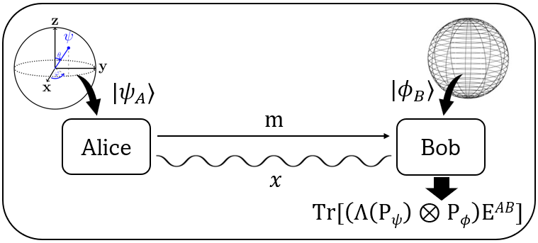
Channel simulation, generic setup.– The simulation of a quantum channel must faithfully reproduce all possible measurement outcome statistics as dictated by the Born rule. This encompasses broader scenario of channel simulation that involves reproducing the statistics of a joint measurement , applied to system , known to Alice, and system , provided to Bob (see Fig. 1). Importantly, the state of system may be unknown to both parties and could even form part of a larger entangled system, such as . This generalized context introduces significant challenges for classical simulation protocols. The communication cost for such a simulation, denoted as , can be defined analogously to simpler scenarios but incorporates the additional complexity of joint measurements and entanglement. As a relevant aside, here we recall the semi-quantum Bell scenario introduced in [53]. In the traditional bipartite Bell game, spacelike-separated Alice and Bob generate classical outputs and in response to classical inputs and , producing an input-output probability distribution . In contrast, the semi-quantum Bell scenario replaces these classical inputs with quantum states and , which may be unknown to the players. This framework has revealed the nonlocality of all entangled quantum states [53] and has spurred various applications [54, 55, 56, 57]. The quantumness of preparation also find application in verifiability of blind quantum computation [58, 59, 60]. Coming back to the generalized channel simulation problem, we establish that the minimum communication cost diverges to infinity, even for the case of qubit channels.
Theorem 1.
The generic simulation of the perfect qubit channel is fundamentally impossible using classical resources alone, even if Alice is permitted to send an arbitrary but finite amount of classical information to Bob.
Proof.
Consider that the classical description of a qubit state, , is provided to Alice. Meanwhile, Bob is provided with another qubit state , which is unknown to both Alice and Bob. While generic simulation requires reproducing the statistics of all possible POVMs performed on the joint state even when the POVM is not known to Alice, let us focus on a specific measurement, only; where is the singlet state. According to the Born rule, the probability of obtaining the outcome is given by:
| (1) |
The most general classical protocol that Alice and Bob can implement to simulate the statistics in Eq. (1) proceeds as follows: Alice generates a classical variable , sampled according to the conditional distribution , where is a shared random variable sampled as , and is the state given to Alice, uniformly sampled from the Bloch sphere; Alice communicates to Bob; Bob performs a two-outcome POVM on the unknown state . Since is unknown to both parties, their protocols are independent of . Associating with the outcome in Eq. (1), perfect simulation demands:
where is the effective POVM element implemented by Bob on , given that Alice is provided with .
Consider now the case where , leading to , which implies , with for all ; here denotes the state orthonormal to , with . Next, consider the case where ; here, , implying for all . Thus, whenever Alice is given the state , Bob’s effective POVM on must take the form . Since is uniformly sampled from the Bloch sphere and is unknown to Bob, no classical protocol involving only a finite amount of classical communication from Alice to Bob can achieve the desired outcome. This completes the proof. ∎
A natural question is whether the use of entangled basis measurements is essential to establish the no-go result in Theorem 1. Specifically, if the joint measurement consists solely of product or separable effects, can its statistics be simulated with finite communication? To address this question we start by observing that the statistics of computational basis measurements, , can be simulated using only 1 bit of classical communication from Alice to Bob: Alice measures her state in basis and communicates measurement outcome to Bob, who also measures his unknown state in basis. A similar approach works for the twisted measurement : Alice measures her state in basis and communicates the result to Bob, who performs either or measurement on his qubit, depending on Alice’s communication. The simulation becomes slightly more intricate when the twist is on Alice’s side, namely for the measurement . In this case, Alice performs measurements in both the and bases on her state and sends the outcomes to Bob using two separate 1-bit classical channels. This is possible as the state is known to her, and thus she can make copies of it. Bob measures his qubit in the basis and selects the appropriate bit from Alice’s communication based on his measurement result. These observations leads us to the following general result.
Theorem 2.
Statistics of any product von Neumann measurement on a qubit, known to Alice, and an unknown qudit held by Bob can always be simulated at Bob’s end by finite classical communication from Alice to Bob.
Proof.
It is known that any product von Neumann measurement in are implementable under LOCC [61]. Proof of our theorem follows a similar reasoning as of there. A generic orthonormal product Basis (OPB) of takes the form , with
| (2) |
where, and for , . Notably, the subspaces at Bob’s part are mutually orthogonal. To simulate the statistic of von Neumann measurement on the basis they apply the following protocol: (i) Bob performs a measurement distinguishing the subspaces ’s, while Alice performs measurements on different copies of her known state, and through different classical channels she communicates whenever the projector clicks; (ii) Bob considers the communication from channel if his projector corresponding to subspace clicks, and then he performs a measurement that distinguishes the states if Alice’s communication is , otherwise he performs a measurement that distinguishes the states . This completes the protocol with an explicit example discussed in Supplemental material. ∎
Although simulation of the twisted measurement can be achieved with 1 bit of communication from Alice to Bob, discussion on simulability of product von Neumann measurement we end with the following observation.
Observation 1.
Outcome statistics of on Alice’s known qubit and Bob’s unknown qubit cannot be reproduce at Bob’s laboratory with 1 bit of communication from Alice.
The proof is obtained utilizing the fact that in random-access-code (RAC) task, a qubit provides an advantage over the classical bit [62, 63] (see Appendix I).
Theorem 2, however, does not fully resolve the question of whether all product POVMs can be simulated with a finite amount of classical communication from Alice to Bob, as there exist measurements involving only rank-1 product effects, but not LOCC implementable. For instance, inspired by an construction in [64], we consider the following POVM:
| (3) |
where . We call this the twisted-butterfly POVM , a name justified by its structure (see Fig.2).
Lemma 1.
The POVM is not implementable by Alice and Bob under the operational paradigm of LOCC.
Proof.
Although the measurement is not LOCC implementable, quite interestingly, it turns out that the statistics of this measurement on a qubit state known to Alice and an unknown qubit state provided to Bob can be simulated at Bob’s end with finite classical communication from Alice. Instead of proving this particular claim, in the following we establish a more generic result (proof provide in Appendix II).
Theorem 3.
Statistics of any separable measurement on a quantum state known to Alice and an unknown state of another quantum system provided to Bob, can always be simulated at Bob’s end by finite classical communication from Alice to Bob.
Theorem 3 is important as it establishes that the no-go result in Theorem 1 necessitates considering a measurement involving entangled effects on the joint system of Alice and Bob. In Supplemental material we argue that statistics of the measurement can be simulated at Bob’s end by 1-bit of communication from Alice.
Remark 1.
The 1-bit classical simulation of highlights a fundamental distinction between the simulation of measurement statistics and its implementation under LOCC. While is not implementable via LOCC (Lemma 1), its statistics can still be simulated using only 1 bit of communication. Conversely, the measurement , though LOCC-implementable, requires more than 1 bit of communication to simulate its statistics (Observation 1).
Simulating noisy qubit channels.– Thus far, we have focused on the simulation of perfect qubit channel. A natural extension is to ask whether the no-go result of Theorem 1 applies to imperfect qubit channels. To address this, we consider the qubit depolarizing channel , defined as , where . We now analyze the classical simulability of this particular class of channels.
Theorem 4.
For all , the qubit depolarizing channel can be simulated with a finite amount of classical communication from Alice to Bob. The required communication increases as .
Proof.
Given a known state , if Alice can ensure that the state is reproduced at Bob’s laboratory, then any generic measurement statistics can also be reproduced by Bob. Let Alice be allowed to communicate classical bits to Bob. To reproduced the state at Bob’s end their protocol proceeds as follows:- (i) Shared Randomness: Alice and Bob share a classical random variable , which is drawn Haar-randomly from the set of unitary operators on . (ii) Predefined States: Before the protocol begins, Alice and Bob agree on a set of equally spaced Bloch vectors with the corresponding qubit states . (iii) Overlap Computation and Communication: Given the input state , Alice computes the overlaps for all and identifies the index that maximizes this overlap. She communicates the index to Bob using -bit classical communication. (iv) State Preparation at Bob’s End: Upon receiving and having access to the shared variable , Bob prepares the state . As shown in the Appendix III, on average the state is prepared at Bob’s laboratory. The parameter approaches unity as the number of bits increases, thus allowing increasingly accurate simulation of the depolarizing channel. ∎
In general, deriving an exact expression for for arbitrary is challenging, as it depends on the specific choices of Bloch vectors . However, for small ’s we can have some natural choices of Bloch vectors – =: 2 diametrically opposite vectors, yielding and , =: 4 vectors forming a regular tetrahedron, yielding and , and =: 8 vectors forming the vertices of a cube, yielding and .
Discussions.– We have generalized the channel simulation task which has a long history in literature [43, 41, 40, 42, 44]. While the standard simulation scenario allows efficient classical protocols, in the generalized task we have shown that simulation of a perfect qubit channel requires an unbounded amount of classical communication from Alice to Bob, even when augmented with arbitrary pre-shared classical correlation. In particular, even though Alice has complete classical knowledge of her qubit state, the unknown state provided to Bob prohibits an efficient classical simulation.
This finding raises some deep foundational questions. For instance, in the standard simulation scenario, it has been shown that simulating any POVM at Bob’s end with finite classical communication from Alice is possible if and only if there exists a -epistemic model underlying quantum theory, where quantum wavefunctions represent an agent’s knowledge about the system [43]. Extension of this result to the generalized simulation scenario along with our no-go results (Theorems 1) would suggest a -ontic nature of the qubit wavefunction. That is, wavefunctions correspond to intrinsic properties of the system rather than merely an observer’s knowledge. Such a conclusion would align with the claims of the Pusey-Barrett-Rudolph (PBR) theorem [66]. Additionally, it would offer a pathway to weaken the Preparation Independence assumption used in the PBR theorem, an assumption that has faced criticism [67]. On the other hand, inspired by studies like [68], it would be intriguing to examine the status of Theorem 1 when Bob’s unknown state is restricted to a predefined set.
Acknowledgements.
Authors acknowledge the conference “Observing a Century of Quantum Mechanics" held at IISER Kolkata, where initial discussion of this project started. SGN acknowledges support from the CSIR project -EMR-I. NG acknowledges support from the NCCR SwissMap. MB acknowledges funding from the National Mission in Interdisciplinary Cyber-Physical systems from the Department of Science and Technology through the I-HUB Quantum Technology Foundation (Grant no: I-HUB/PDF/2021-22/008).I Appendix-I: Proof of Observation 1
Proof.
We start by recalling the RAC task [62, 63], where Alice is provided with a random bit string and Bob is randomly given . Bob’s aim to produce a 1-bit outcome with the help of 1-bit respectively 1-qubit communication from Alice. Qubit strategies yield the optimal success which is strictly higher than the optimal c-bit success .
Contrary to the claim of the Observation 1, let us assume that the statistics of the measurement on a state known to Alice and an unknown state of Bob system can be simulated at Bob’s end with just 1-bit of classical communication from Alice to Bob. Let us denote this protocol as -. As we will argue now, this protocol can be utilized to perform the RAC task. Given the bit string Alice will implement the - protocol on the preparation
| (4) |
whereas Bob, given the question , will prepare the state
| (5) |
As per the assumption, - protocol reproduce the statistics of on at Bob’s laboratory. Bob can post-process this outcome statistics and can accordingly devise a strategy to answer his guess . In particular, for the outcomes and Bob guesses , else he guesses . Denoting and , we have
| (6) |
Therefore, with - protocol one can have a success in RAC task – a contradiction. In other words, this proves that with 1-bit communication the statistics of cannot be reproduced at Bob’s laboratory. ∎
II Appendix-II: Proof of Theorem 3
We start by recalling a definition from [69] (see Section 2.3.3 in page 113).
Definition 1.
[Rank-1 extremal POVM] A outcome POVM is called rank-1 extremal POVM if for all , with being a rank-1 projector, and implies ; or equivalently all nonzero elements in are linearly independent of each other. Let, denotes the set of all rank-1 extremal POVMs.
The notion of rank-1 extremal POVMs leads us to the following useful Lemma.
Lemma 2.
Any finite element rank-1 POVM can be written as probabilistic mixture of finite number of rank-1 extremal POVMs, i.e., , with and .
Proof.
Consider an arbitrary rank-1 POVM with finite outcomes , with . According to Definition 1, allows convex decomposition in terms of , i.e.
| (7) |
being a rank-1 projector it follows that , whenever . On the other hand, for also we can assume , which thus implies . Thus we have . For such an we can define . The extremality of implies the set of effects to be linearly independent, and furthermore the condition uniquely specifies the values of ’s for any . As the set contains finitely many projectors, there are only finitely many ways of choosing such that turns out to be a rank-1 extremal POVM. Therefore, the integral in Eq.(7) gets replaced by finite summation, meaning
| (8) |
This completes the proof. ∎
Proof of Theorem 3:-.
Proof.
Since any separable POVM is coarse-graining of rank-1 product POVMs, it suffices to prove our claim for the later only. Consider an outcomes rank-1 product POVM
| (9) |
Given a known state to Alice and an unknown state to Bob, they aim to reproduce the outcome statistics
| (10) |
at Bob’s laboratory. Denoting , the statistics in Eq.(10) can be view as the outcome statistics of the the effective rank-1 POVM on Bob’s unknown state . Lemma 2 ensures that POVM can be expressed as probabilistic mixture of finite number of rank-1 extremal POVMs , i.e.
| (11) |
More specifically Eq.(11) depicts that the coefficients in convex mixture depend on the state of Alice’s system. To simulate the statistics of Eq.(10) at Bob’s end, Alice given a known state generates a random variable according to probability distribution and communicates it to Bob using -bits of classical communication. Upon receiving the random variable Bob implements the corresponding rank-1 extremal POVM on his unknown state . This completes the protocol. ∎
In Supplemental material, we detail the aforementioned protocol for twisted-butterfly POVM.
III Appendix-III: Detailed proof of Theorem 4
Given the state , the protocol ensures that the state , prepared at Bob’s end, lies within the cone forming an apex angle with the vector . Furthermore, since the random variable is drawn Haar-randomly from the set of unitaries acting on , all the states within this cone are prepared with equal probability. Consequently, on average, Bob prepares a resulting density operator , with .
Denoting the Bloch vector of as , the components of the resulting density operator are given by:
| (12a) | ||||
| (12b) | ||||
| (12c) | ||||
For instance, if Alice is given the state , then the components of the Bloch vector for Bob’s resulting state are:
Thus, the resulting density operator at Bob’s end is:
| (13) |
The above calculation yields the same result for any arbitrary state provided to Alice, confirming that the protocol simulates a depolarizing channel with parameter . Notably, as increases, decreases, and increases. In the limiting case , we have and , which aligns with the claims of Theorem 1. Thus, for any value of , a simulation is always achievable with bits of finite communication, provided is sufficiently large.
References
- Gisin [2019] N. Gisin, Indeterminism in Physics, Classical Chaos and Bohmian Mechanics: Are Real Numbers Really Real?, Erkenntnis 86, 1469–1481 (2019).
- Dirac [1930] P. M. A. Dirac, The Principles of Quantum Mechanics (Clarendon Press, Oxford,, 1930).
- von Neumann [2018] J. von Neumann, Mathematical Foundations of Quantum Mechanics: New Edition (Princeton University Press, 2018).
- Peres [2002] A. Peres, Quantum Theory: Concepts and Methods (Springer Netherlands, 2002).
- Deutsch and Jozsa [1992] D. Deutsch and R. Jozsa, Rapid solution of problems by quantum computation, Proc. R. Soc. Lond. A 439, 553 (1992).
- [6] P. Shor, Algorithms for quantum computation: discrete logarithms and factoring, in Proceedings 35th Annual Symposium on Foundations of Computer Science, SFCS-94 (IEEE Comput. Soc. Press) p. 124–134.
- Grover [1996] L. K. Grover, A fast quantum mechanical algorithm for database search, in Proceedings of the twenty-eighth annual ACM symposium on Theory of computing - STOC ’96, STOC ’96 (ACM Press, 1996) p. 212–219.
- Bennett and Wiesner [1992] C. H. Bennett and S. J. Wiesner, Communication via one- and two-particle operators on Einstein-Podolsky-Rosen states, Phys. Rev. Lett. 69, 2881 (1992).
- Bennett et al. [1993] C. H. Bennett, G. Brassard, C. Crépeau, R. Jozsa, A. Peres, and W. K. Wootters, Teleporting an unknown quantum state via dual classical and Einstein-Podolsky-Rosen channels, Phys. Rev. Lett. 70, 1895 (1993).
- Buhrman et al. [2010] H. Buhrman, R. Cleve, S. Massar, and R. de Wolf, Nonlocality and communication complexity, Rev. Mod. Phys. 82, 665 (2010).
- Bennett and Brassard [2014] C. H. Bennett and G. Brassard, Quantum cryptography: Public key distribution and coin tossing, Theo. Compu. Sc. 560, 7–11 (2014).
- Ekert [1991] A. K. Ekert, Quantum cryptography based on Bell’s theorem, Phys. Rev. Lett. 67, 661 (1991).
- Gisin et al. [2002] N. Gisin, G. Ribordy, W. Tittel, and H. Zbinden, Quantum cryptography, Rev. Mod. Phys. 74, 145 (2002).
- Feynman [1982] R. P. Feynman, Simulating physics with computers, Int. J. Theo. Phys. 21, 467–488 (1982).
- Bremner et al. [2010] M. J. Bremner, R. Jozsa, and D. J. Shepherd, Classical simulation of commuting quantum computations implies collapse of the polynomial hierarchy, Proc. R. Soc. London A 467, 459–472 (2010).
- Rahimi-Keshari et al. [2016] S. Rahimi-Keshari, T. C. Ralph, and C. M. Caves, Sufficient Conditions for Efficient Classical Simulation of Quantum Optics, Phys. Rev. X 6, 021039 (2016).
- Bell [1964] J. S. Bell, On the Einstein Podolsky Rosen paradox, Physics Physique Fizika 1, 195 (1964).
- Freedman and Clauser [1972] S. J. Freedman and J. F. Clauser, Experimental Test of Local Hidden-Variable Theories, Phys. Rev. Lett. 28, 938 (1972).
- Aspect et al. [1981] A. Aspect, P. Grangier, and G. Roger, Experimental Tests of Realistic Local Theories via Bell’s Theorem, Phys. Rev. Lett. 47, 460 (1981).
- Aspect et al. [1982a] A. Aspect, P. Grangier, and G. Roger, Experimental Realization of Einstein-Podolsky-Rosen-Bohm Gedankenexperiment: A New Violation of Bell’s Inequalities, Phys. Rev. Lett. 49, 91 (1982a).
- Aspect et al. [1982b] A. Aspect, J. Dalibard, and G. Roger, Experimental Test of Bell’s Inequalities Using Time-Varying Analyzers, Phys. Rev. Lett. 49, 1804 (1982b).
- Zukowski et al. [1993] M. Zukowski, A. Zeilinger, M. A. Horne, and A. K. Ekert, “event-ready-detectors” Bell experiment via entanglement swapping, Phys. Rev. Lett. 71, 4287 (1993).
- Tittel et al. [1998] W. Tittel, J. Brendel, H. Zbinden, and N. Gisin, Violation of Bell Inequalities by Photons More Than 10 km Apart, Phys. Rev. Lett. 81, 3563 (1998).
- Weihs et al. [1998] G. Weihs, T. Jennewein, C. Simon, H. Weinfurter, and A. Zeilinger, Violation of Bell’s Inequality under Strict Einstein Locality Conditions, Phys. Rev. Lett. 81, 5039 (1998).
- Bell [1966] J. S. Bell, On the Problem of Hidden Variables in Quantum Mechanics, Rev. Mod. Phys. 38, 447 (1966).
- Mermin [1993] N. D. Mermin, Hidden variables and the two theorems of John Bell, Rev. Mod. Phys. 65, 803 (1993).
- Aspect [2002] A. Aspect, Bell’s Theorem: The Naive View of an Experimentalist, in Quantum [Un]speakables (Springer Berlin Heidelberg, 2002) p. 119–153.
- Brunner et al. [2014] N. Brunner, D. Cavalcanti, S. Pironio, V. Scarani, and S. Wehner, Bell nonlocality, Rev. Mod. Phys. 86, 419 (2014).
- Gisin [2023] N. Gisin, Quantum non-locality: from denigration to the nobel prize, via quantum cryptography, Europhysics News 54, 20–23 (2023).
- Horodecki et al. [2009] R. Horodecki, P. Horodecki, M. Horodecki, and K. Horodecki, Quantum entanglement, Rev. Mod. Phys. 81, 865 (2009).
- Brassard et al. [1999] G. Brassard, R. Cleve, and A. Tapp, Cost of Exactly Simulating Quantum Entanglement with Classical Communication, Phys. Rev. Lett. 83, 1874 (1999).
- Steiner [2000] M. Steiner, Towards quantifying non-local information transfer: finite-bit non-locality, Phys. Lett. A 270, 239–244 (2000).
- Massar et al. [2001] S. Massar, D. Bacon, N. J. Cerf, and R. Cleve, Classical simulation of quantum entanglement without local hidden variables, Phys. Rev. A 63, 052305 (2001).
- Regev and Toner [2010] O. Regev and B. Toner, Simulating Quantum Correlations with Finite Communication, SIAM Journal on Computing 39, 1562–1580 (2010).
- Branciard and Gisin [2011] C. Branciard and N. Gisin, Quantifying the Nonlocality of Greenberger-Horne-Zeilinger Quantum Correlations by a Bounded Communication Simulation Protocol, Phys. Rev. Lett. 107, 020401 (2011).
- Kar et al. [2011] G. Kar, M. R. Gazi, M. Banik, S. Das, A. Rai, and S. Kunkri, A complementary relation between classical bits and randomness in local part in the simulating singlet state, J. Phys. A: Math. Theo. 44, 152002 (2011).
- Branciard et al. [2012] C. Branciard, N. Brunner, H. Buhrman, R. Cleve, N. Gisin, S. Portmann, D. Rosset, and M. Szegedy, Classical Simulation of Entanglement Swapping with Bounded Communication, Phys. Rev. Lett. 109, 100401 (2012).
- Banik et al. [2012] M. Banik, M. R. Gazi, S. Das, A. Rai, and S. Kunkri, Optimal free will on one side in reproducing the singlet correlation, J. Phys. A: Math. Theo. 45, 205301 (2012).
- Roy et al. [2014] A. Roy, A. Mukherjee, S. S. Bhattacharya, M. Banik, and S. Das, Local deterministic simulation of equatorial von neumann measurements on tripartite ghz state, Quant. Inf. Processing 14, 217–228 (2014).
- Cerf et al. [2000] N. J. Cerf, N. Gisin, and S. Massar, Classical Teleportation of a Quantum Bit, Phys. Rev. Lett. 84, 2521 (2000).
- Toner and Bacon [2003] B. F. Toner and D. Bacon, Communication Cost of Simulating Bell Correlations, Phys. Rev. Lett. 91, 187904 (2003).
- Methot [2004] A. A. Methot, Simulating POVMs on EPR pairs with 5.7 bits of expected communication, EPJD 29, 445–446 (2004).
- Montina [2012] A. Montina, Epistemic View of Quantum States and Communication Complexity of Quantum Channels, Phys. Rev. Lett. 109, 110501 (2012).
- Renner et al. [2023] M. J. Renner, A. Tavakoli, and M. T. Quintino, Classical Cost of Transmitting a Qubit, Phys. Rev. Lett. 130, 120801 (2023).
- Kraus [1983] K. Kraus, States, Effects, and Operations: Fundamental Notions of Quantum Theory (Springer Berlin Heidelberg, 1983).
- [46] A quantum channel from Alice to Bob is a linear map ; where denotes the space of linear operators on the corresponding Hilbert space. Positivity of the map demands ; and complete positivity demands positivity of forall , where denotes the identity map on the operator space of dimensional Hilbert space, .
- Lo [2000] H.-K. Lo, Classical-communication cost in distributed quantum-information processing: A generalization of quantum-communication complexity, Phys. Rev. A 62, 012313 (2000).
- Pati [2000] A. K. Pati, Minimum classical bit for remote preparation and measurement of a qubit, Phys. Rev. A 63, 014302 (2000).
- Bennett et al. [2001] C. H. Bennett, D. P. DiVincenzo, P. W. Shor, J. A. Smolin, B. M. Terhal, and W. K. Wootters, Remote State Preparation, Phys. Rev. Lett. 87, 077902 (2001).
- Harsha et al. [2010] P. Harsha, R. Jain, D. McAllester, and J. Radhakrishnan, The Communication Complexity of Correlation, IEEE Trans. Inf. Theory 56, 438–449 (2010).
- Winter [2002] A. Winter, Compression of sources of probability distributions and density operators, arXiv:quant-ph/0208131 (2002).
- Kochen and Specker [1967] S. Kochen and E. Specker, The Problem of Hidden Variables in Quantum Mechanics, J. Math. Mech. 17, 59–87 (1967).
- Buscemi [2012] F. Buscemi, All Entangled Quantum States Are Nonlocal, Phys. Rev. Lett. 108, 200401 (2012).
- Branciard et al. [2013] C. Branciard, D. Rosset, Y.-C. Liang, and N. Gisin, Measurement-Device-Independent Entanglement Witnesses for All Entangled Quantum States, Phys. Rev. Lett. 110, 060405 (2013).
- Banik [2013] M. Banik, Lack of measurement independence can simulate quantum correlations even when signaling can not, Phys. Rev. A 88, 032118 (2013).
- Chaturvedi and Banik [2015] A. Chaturvedi and M. Banik, Measurement-device–independent randomness from local entangled states, EPL 112, 30003 (2015).
- Lobo et al. [2022] E. P. Lobo, S. G. Naik, S. Sen, R. K. Patra, M. Banik, and M. Alimuddin, Certifying beyond quantumness of locally quantum no-signaling theories through a quantum-input Bell test, Phys. Rev. A 106, L040201 (2022).
- Childs [2005] A. Childs, Secure assisted quantum computation, Quantum Inf. Comput. 5, 456–466 (2005).
- Fitzsimons and Kashefi [2017] J. F. Fitzsimons and E. Kashefi, Unconditionally verifiable blind quantum computation, Phys. Rev. A 96, 012303 (2017).
- Ma et al. [2022] Y. Ma, E. Kashefi, M. Arapinis, K. Chakraborty, and M. Kaplan, QEnclave - A practical solution for secure quantum cloud computing, npj Quantum Information 8, 128 (2022).
- Bennett et al. [1999] C. H. Bennett, D. P. DiVincenzo, T. Mor, P. W. Shor, J. A. Smolin, and B. M. Terhal, Unextendible Product Bases and Bound Entanglement, Phys. Rev. Lett. 82, 5385 (1999).
- Wiesner [1983] S. Wiesner, Conjugate coding, ACM SIGACT News 15, 78–88 (1983).
- Ambainis et al. [2002] A. Ambainis, A. Nayak, A. Ta-Shma, and U. Vazirani, Dense quantum coding and quantum finite automata, Journal of the ACM 49, 496–511 (2002).
- Duan et al. [2009] R. Duan, Y. Feng, Y. Xin, and M. Ying, Distinguishability of Quantum States by Separable Operations, IEEE Tran. Inf. Theory 55, 1320–1330 (2009).
- Walgate and Hardy [2002] J. Walgate and L. Hardy, Nonlocality, Asymmetry, and Distinguishing Bipartite States, Phys. Rev. Lett. 89, 147901 (2002).
- Pusey et al. [2012] M. F. Pusey, J. Barrett, and T. Rudolph, On the reality of the quantum state, Nature Physics 8, 475–478 (2012).
- Schlosshauer and Fine [2014] M. Schlosshauer and A. Fine, No-go Theorem for the Composition of Quantum Systems, Phys. Rev. Lett. 112, 070407 (2014).
- Henderson et al. [2000] L. Henderson, L. Hardy, and V. Vedral, Two-state teleportation, Phys. Rev. A 61, 062306 (2000).
- Watrous [2018] J. Watrous, The Theory of Quantum Information (Cambridge University Press, 2018).
SUPPLEMENTAL MATERIAL
IV Theorem 2: An Explicit Example
For a better clarification of Theorem 2, here we provide an explicit example. Consider the OPB of system, where
| (14a) | ||||
| (14b) | ||||
| (14c) | ||||
with, and . To simulate statistics of the measurement on this basis, Bob, on his unknown state, first performs a measurement consisting of three rank-2 projective effects
| (15) |
On the other hand, Alice performs , , and measurements on three copies of her known state, and communicates the outcomes through three 1-bit classical channels, respectively , , and , to Bob. Depending on which projector clicks in his first measurement, Bob chooses the corresponding communication line from Alice, and depending on the communication received from Alice, he performs the measurements as shown is Table 1.
| Outcome of | Selected Channel | Communication | Bob’s final measurement | |
|---|---|---|---|---|
| Channel | ||||
| Channel | ||||
| Channel | ||||
This protocol exactly reproduces the measurement statistics at Bob’s end, while utilizing three classical bits from Alice.
V Classical Simulation of twisted-Butterfly POVM
The twisted-Butterfly POVM induces the following effective POVM on Bob’s part:
| (16) |
where denotes the component of the Bloch vector of of Alice’s known state . Using the four projectors one can obtain only four rank-1 extremal POVMs, namely
| (17) |
The POVM allows a convex decomposition in terms of extremal POVMs , i.e.
| (18a) | ||||
| (18b) | ||||
To simulate statistics of twisted-butterfly POVM, Alice after receiving classical description of the state communicates a four valued random variable sampled according to a distribution , and then Bob according performs the measurement on his unknown state . Thus 2 bits of communication channel is required from Alice to Bob to implement this classical protocol.
Notably, for , a more efficient classical simulation is possible. Since, and for all , the also allows following convex decomposition in terms of two non extremal rank-1 POVMs,
| (19a) | ||||
| (19b) | ||||
Alice thus sends two-valued random variable sampled according to the distribution , and Bob accordingly performs the measurement or on his unknown qubit. This protocol exactly reproduce the required statistics at Bob’s end with 1-bit of classical communication from Alice.