Non-asymptotic convergence bounds for
Wasserstein approximation using point clouds
Abstract
Several issues in machine learning and inverse problems require to generate discrete data, as if sampled from a model probability distribution. A common way to do so relies on the construction of a uniform probability distribution over a set of points which minimizes the Wasserstein distance to the model distribution. This minimization problem, where the unknowns are the positions of the atoms, is non-convex. Yet, in most cases, a suitably adjusted version of Lloyd’s algorithm — in which Voronoi cells are replaced by Power cells — leads to configurations with small Wasserstein error. This is surprising because, again, of the non-convex nature of the problem, as well as the existence of spurious critical points. We provide explicit upper bounds for the convergence speed of this Lloyd-type algorithm, starting from a cloud of points sufficiently far from each other. This already works after one step of the iteration procedure, and similar bounds can be deduced, for the corresponding gradient descent. These bounds naturally lead to a modified Poliak-Łojasiewicz inequality for the Wasserstein distance cost, with an error term depending on the distances between Dirac masses in the discrete distribution.
1 Introduction
In recent years, the theory of optimal transport has been the source of stimulating ideas in machine learning and in inverse problems. Optimal transport can be used to define distances, called Wasserstein or earth-mover distances, between probability distributions over a metric space. These distances allows one to measure the closeness between a generated distribution and a model distribution, and they have been used with success as data attachment terms in inverse problems. Practically, it has been observed for several different inverse problems that replacing usual loss functions with Wasserstein distances tend to increase the basin of convergence of the methods towards a good solution of the problem, or even to convexify the landscape of the minimized energy [7, 6]. This good behaviour is not fully understood, but one may attribute it partly to the fact that the Wasserstein distances encodes the geometry of the underlying space. A notable use of Wasserstein distances in machine learning is in the field of generative adversarial networks, where one seeks to design a neural network able to produce random examples whose distribution is close to a prescribed model distribution [2].
Wasserstein distance and Wasserstein regression
Given two probability distributions on , the Wasserstein distance of exponent between and is a way to measure the total cost of moving mass distribution described by to , knowing that moving a unit mass from to costs . Formally, it is defined as the value of an optimal transport problem between and :
| (1) |
where we minimize of the set of transport plans between and , i.e. probability distributions over with marginals and . Standard references on the theory of optimal transport include books by Villani and by Santambrogio [19, 20, 18], while the computational and statistical aspects are discussed in a survey of Cuturi and Peyré [16].
In this article, we consider regression problems with respect to the Wasserstein metric, which can be put in the following form
| (2) |
where is the reference distribution, a probability measure on , is the model distribution, a probability measure on , and where is a family of maps indexed by a parameter . In the previous formula, we also denoted the image of the measure under the map , also called pushforward of under . This image measure is defined by for any measurable set in the codomain of . In this work, we will concentrate on the quadratic Wasserstein distance . Several problems related to the design of generative models can be put under the form (2), see for instance [8, 2]. Solving (2) numerically is challenging for several reasons, but in this article we will concentrate on one of them: the non-convexity of the Wasserstein distance under displacement of the measures.
Non-convexity of the Wasserstein distance under displacements.
It is well known that the Wasserstein distance is convex for the standard (linear) structure of the space of probability measures, meaning that if and are two probability measures and , then the map is convex. Using a terminology from physics, we may say that the Wasserstein distance is convex for the Eulerian structure of the space of probability measures, e.g. when one interpolates linearly between the densities. However, in the regression problem (2), the perturbations are Lagrangian rather than Eulerian, in the sense that modifications of the parameter leads to a displacement of the support of the measure . This appears very clearly in particular when is the uniform measure over a set of point in , i.e. with
In this case is the uniform measure over the set , i.e. . In this article, we will therefore be interested by the function
| (3) |
This function is not convex, and actually exhibits (semi-)concavity properties. This has been observed first in [1] (Theorem 7.3.2), and is related to the positive curvature of the Wasserstein space. A precise statement in the context considered here may also be found as Proposition 21 in [14]. A practical consequence of the lack of convexity of is that critical points of are not necessarily global minimizers. It is actually easy to construct examples families of critical points of such that is bounded from below by a positive constant, while , so that the ratio between and is arbitrarily large as . This can be done by concentrating the points on lower-dimensional subspaces of , as in Remarks 2 and 3.
When applying gradient descent to the nonconvex optimization problem (2), it is in principle possible to end up on local minima corresponding to a high energy critical points of the Wasserstein distance, regardless of the non-linearity of the map . Our main theorem, or rather its Corollary 6 shows that if the points of are at distance at least from one another, then
In the previous equation denotes the Euclidean norm of the vector in obtained by putting one after the other the gradients of w.r.t. the positions of the atoms . We note that due to the weights in the atomic measure , the components of this vector are in general of the order of , see Proposition 1. This inequality resembles the Polyak-Łojasiewicz inequality, and shows in particular that if the quantization error is large, i.e. larger than , then the point cloud is not critical for . From this, we deduce in 7 that if the points in the initial cloud are not too close to each other at the initialization, then the iterates of fixed step gradient descent converge to points with low energy , despite the non-convexity of .
|

|
|
|
Relation to optimal quantization
Our main result also has implications in terms of the uniform optimal quantization problem, where one seeks a point cloud in such that the uniform measure supported over , denoted , is as close as possible to the model distribution with respect to the -Wasserstein distance:
| (4) |
The uniform optimal quantization problem (4) is a very natural variant of the (standard) optimal quantization problem, where one does not impose that the measure supported on is uniform:
| (5) |
and where is the probability simplex. This standard optimal quantization problem is a cornerstone of sampling theory, and we refer the reader to the book of Graf and Luschgy [10] and to the survey by Pagès [15]. The uniform quantization problem (4) is less common, but also very natural. It has been used in imaging to produce stipplings of an image [4, 3] or for meshing purposes [9]. A common difficulty for solving (5) and (4) numerically is that the minimized functionals and are non-convex and have many critical points with high energy. However, in practice, simple fixed-point or gradient descent stategies behave well when the initial point cloud is not chosen adversely. Our second contribution is a quantitative explanation for this good behaviour in the case of the uniform optimal quantization problem.
Lloyd’s algorithm [12] is a fixed point algorithm for solving approximately the standard optimal quantization problem (5). Starting from a point cloud with distinct points, one defines the next iterate in two steps. First, one computes the Voronoi diagram of , a tessellation of the space into convex polyhedra , where
| (6) |
In the second step, one moves every point towards the barycenter, with respect to , of the corresponding cell . This algorithm can also be interpreted as a fixed point algorithm for solving the first-order optimality condition for (5), i.e. . One can show that the energy decreases in . The convergence of towards a critical point of as has been studied in [5], but the energy of this limit critical point is not guaranteed to be small.
In the case of the uniform quantization problem (4), one can try to minimize the energy by gradient descent, defining the iterates
| (7) |
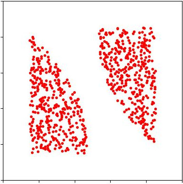
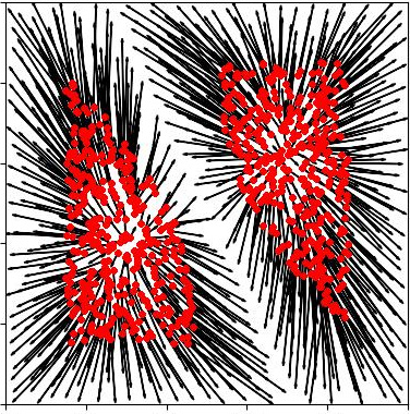
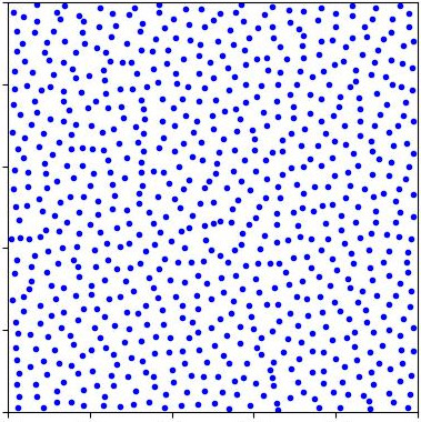
where is the time step. The factor in front of is set as a compensation for the fact that we have, in general, . When , one recovers a version of Lloyd’s algorithm for the uniform quantization problem, involving barycenters of Power cells, rather than Voronoi cells, associated to . More precisely, Proposition 1 proves that so that when . Quite surprisingly, we prove in Corollary 4 that if the points in the initial cloud are not too close to each other, then the uniform measure over the point cloud obtained after only one step of Lloyd’s algorithm is close to . This is illustrated in Figure 1. We prove in particular the following statement.
Theorem (Particular case of Corollary 4).
Let be a probability density over a compact convex set , let and assume that the points lie at some positive distance from one another: for some constant ,
corresponding for instance to a point cloud sampled on a regular grid. Then, the point cloud obtained after one step of Lloyd’s algorithm satisfies
where is a constant depending on and .
Outline
In Section 2, we start by a short review of background material on optimal transport and optimal uniform quantization. We then establish our main result (3) on the approximation of a measure by barycenters of Power cells. This theorem yields error estimates for one step of Lloyd’s algorithm in deterministic and probabilistic settings (Corollaries 4 and 5). In Section 3, we establish a Polyak-Łojasiewicz-type inequality (Corollary 6) for the function introduced in (3), and we study the convergence of a gradient descent algorithm for (Theorem 7). Finally, in Section 4, we report numerical results on optimal uniform quantization in dimension .
2 Lloyd’s algorithm for optimal uniform quantization
Optimal transport and Kantorovich duality
In this section we briefly review Kantorovich duality and its relation to semidiscrete optimal transport. The cost is fixed to , and we assume that is a probability density over a compact convex domain . In this setting, Brenier’s theorem implies that given any probability measure supported on , the optimal transport plan between and , i.e. the minimizer in the definition of the Wasserstein distance (1) with , is induced by a transport map , meaning . One can derive an alternative expression for the Wasserstein distance using Kantorovich duality, which leads to a more precise description of the optimal transport map [18, Theorem 1.39]:
| (8) |
where . When is the uniform probability measure over a point cloud containing distinct points, we set and we define the th Power cell associated to the couple as
Then, the Kantorovich dual (8) of the optimal transport problem between and turns into a finite-dimensional concave maximization problem
| (9) |
By Corollary 1.2 in [11], a vector is optimal for this maximization problem if and only if the potential is such that each Power cell contain the same amount of mass, i.e. if
| (10) |
From now on, we denote , where satisfies (10). The optimal transport map between and sends every Power cell to the point , i.e. it is defined -almost everywhere by . We refer again to the introduction of [11] for more details.
Optimal uniform quantization
In this article, we study the behaviour of the squared Wasserstein distance between the (fixed) probability density and a uniform finitely supported measure where is a cloud of points, in terms of variations of . As in equation (3), we denote . Proposition 21 in [14] gives an expression for the gradient of , and proves its semiconcavity. We recall that is called –semiconcave, with , if the function is concave. We denote the generalized diagonal
Proposition 1 (Gradient of ).
The function is –semiconcave on and is of class on . In addition, for any one has
| (11) |
and where is the barycenter of the th power cell, i.e. .
It is not difficult to prove that admits at least one minimizer, and that this minimizer satisfies the first-order optimality condition . A point cloud that satisfies this condition is called critical.
Remark 1 (Upper bound on the minimum of ).
We note from [14, Proposition 12] that when is supported on a compact subset of , then
| (12) |
These upper bounds may not be tight, in particular when is separable (see Appendix E).
Remark 2 (High energy critical points).
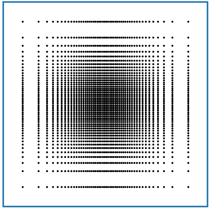
On the other hand, since is not convex, this first-order condition is not sufficient to have a minimizer of . For instance, if on the unit square , one can check that the point cloud
![[Uncaptioned image]](https://cdn.awesomepapers.org/papers/a4b06002-b288-4fac-8638-2c5838888af8/bad_crit_20_recrop.jpg)
is a critical point of but not a minimizer of . In fact, this critical point becomes arbitrarily bad as in the sense that
On the other hand, we note that the point cloud is highly concentrated, in the sense that the distance between consecutive points in is , whereas in an evenly distributed point cloud, one would expect the minimum distance between points to be of order .
Gradient descent and Lloyd’s algorithm
One can find a critical point of by following the discrete gradient flow of , defined in (7), starting from an initial position . Thanks to the expression of given in Proposition 1, the discrete gradient flow may be written as
| (13) |
where is a fixed time step. For , one recovers a variant of Lloyd’s algorithm, where one moves every point to the barycenter of its Power cell at each iteration:
| (14) |
We can state the following result about Lloyd’s algorithm for the uniform quantization problem, whose proof is postponed to the appendix.
Proposition 2.
Let be a fixed integer and be the iterates of (14), with . Then, the energy is decreasing, and . Moreover, the sequence belongs to a compact subset of and every limit point of a converging subsequence of it is a critical point for .
Experiments suggest that following the discrete gradient flow of does not bring us to high energy critical points of , such as those described in Remark 2, unless we started from an adversely chosen point cloud. The following theorem and its corollaries, the main results of this article, backs up this experimental evidence. It shows that if the point cloud is not too concentrated, then the uniform measure over the barycenters of the power cells, , is a good quantization of the probability density , i.e. it bounds the quantization error after one step of Lloyd’s algorithm (14).
We will use the following notation for :
Note that is an -neighborhood around the generalized diagonal .
Theorem 3 (Quantization by barycenters).
Let be a compact convex set, a probability density on and consider a point cloud in . Then, for all ,
| (15) |
where and where is the volume of the unit ball in .
The proof relies on arguments from convex geometry. In particular, we denote the Minkowski sum of sets: .
Proof.
Let be the solution to the dual Kantorovich problem (10) between and . We let and we denote the th Power cell intersected with the slightly enlarged convex set . This way, whereas is in fact the intersection of the -th Voronoi cell defined in (6) with .
We will now prove an upper bound on the sum of the diameters of the cells whose index lies in . First, we notice the following inclusion, which holds for any :
| (16) |
Indeed, let and , so that for all and ,
Expanding the squares and substracting on both sides these inequalities become linear in and , implying directly that as desired.
For any index , the point is at distance at least from other points, implying that is contained in the Voronoi cell with . Using that , that and that , we deduce that contains the same ball. On the other hand, contains a segment of length and inclusion (16) with gives
The Minkowski sum in the left-hand side contains in particular the product of a -dimensional ball of radius with an orthogonal segment with length . Thus,
Using that the Power cells form a tesselation of the domain , we therefore obtain
| (17) |
We now estimate the transport cost between and the density , where . The transport cost due to the points whose indices do not belong to can be bounded in a crude way by
Note that we used . On the other hand, the transport cost associated with indices in can be bounded using (17) and :
In conclusion, we obtain the desired estimate:
This theorem could be extended mutatis mutandis to the case where is a general probability measure (i.e. not a density). However, this would imply some technical complications in the definition of the barycenters by introducing a disintegration of with respect to the transport plan .
Consequence for Lloyd’s algorithm (14)
In the next corollary, we assume that any pair of distinct points in is bounded from below by , implying that . This corresponds to the value one could expect for a point set uniformly sampled from a set with Minkowski dimension . When , the corollary asserts that one step of Lloyd’s algorithm is enough to approximate , in the sense that the uniform measure over the barycenters converges towards as .
Corollary 4 (Quantization by barycenters, asymptotic case).
Assume with . Then, with
| (18) |
and in particular, if ,
| (19) |
Remark 3 (Optimality of the exponent when ).
There is no reason to believe that the exponent in the upper bound (18) is optimal in general. However, it seems to be optimal in a “worst-case sense” when . More precisely, we show the following result in Appendix E: for any , and for every () there exists a sequence of separable probability densities over ( is a truncated Gaussian distributions, whose variance converges to zero slowly as ) such that if is a uniform grid of size in , then
where is independent of . On the other hand, in this setting every point in is at distance at least from any other point in . Applying 4 with , i.e. , we get
Comparing this upper bound on with the above lower bound, one sees that is is not possible to improve the exponent.
Remark 4 (Optimality of (19)).
The assumption for (19) is tight: if is the Lebesgue measure on , it is possible for to construct a point cloud with points on the -cube such that distinct point in are at distance at least . Then, the barycenters are also contained in the cube, so that .
The next corollary is a probabilistic analogue of Corollary 4, assuming that the initial point cloud is drawn from a probability density on . Note that can be distinct from . The proof of this corollary relies on McDiarmid’s inequality to quantify the proportion of -isolated points in a point cloud that is drawn randomly and independently from . The proof of this result is in Appendix B.
Corollary 5 (Quantization by barycenters, probabilistic case).
Let and let be i.i.d. random variables with distribution . Then, there exists a constant depending only on and , such that for large enough,

3 Gradient flow and a Polyak-Łojasiewicz-type inequality
Theorem 3 can be interpred as a modified Polyak-Łojasiewicz-type (PŁ for short) inequality for the function . The usual PŁ inequality for a differentiable function is of the form
where is a positive constant. This inequality has been originally used by Polyak to prove convergence of gradient descent towards the global minimum of . Note in particular that such an inequality implies that any critical point of is a global minimum of . By Remark 2, has critical points that are not minimizers, so that we cannot expect the standard PŁ inequality to hold. What we get is a similar inequality relating and but with a term involving the minimimum distance between the points in place of .
Corollary 6 (Polyak-Łojasiewicz-type inequality).
Let . Then,
| (20) |
We note that when , the term in (20) has order . On the other hand, as recalled in 1, when . Thus, we do not expect (20) to be tight.
Convergence of a discrete gradient flow
The modified Polyak-Łojasiewicz inequality (20) suggests that the discrete gradient flow 13 will bring us close to a point cloud with low Wasserstein distance to , provided that can guarantee that the the points clouds remain far for generalized diagonal during the iterations. We prove in Lemma 3 in Appendix D that if and , then
| (21) |
We note that this inequality ensures that never touches the generalized diagonal , so that the gradient is well-defined at each step. Combining this inequality with 3, one can actually prove that if the points in the initial cloud are not too close to each other, then a few steps of gradient discrete gradient descent leads to a discrete measure that is close to the target . Precisely, we arrive at the following theorem, proved in Appendix D.
Theorem 7.
Let , , and . Let be the iterates of (13) starting from with timestep . We assume that and we set
Then,
| (22) |
Remark 5.
Note that the exponential behavior implied by 21 and 3 is coherent with the estimates that are known in the absolutely continuous setting for the continuous gradient flow. When transitioning from discrete measures to probability densities, lower bounds on the distance between points become upper bounds on the density. The gradient flow has an explicit solution , where is a constant-speed geodesic in the Wasserstein space with and . In this case, a simple adaptation of the estimates in Theorem 2 in [17] shows the bound Still in this absolutely continous setting, it is possible to remove the exponential growth if the target density is also bounded, as a consequence of displacement convexity [13, Theorem 2.2]. There seems to be no discrete counterpart to this argument, explaining in part the discrepancy between the exponent of in (22) with the one obtained in 4.

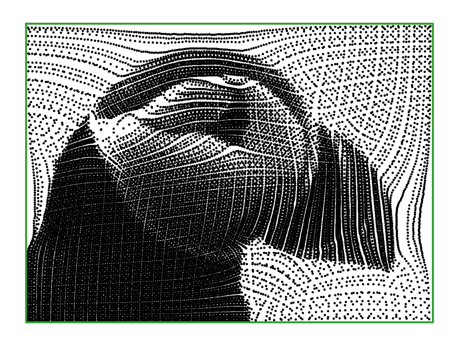
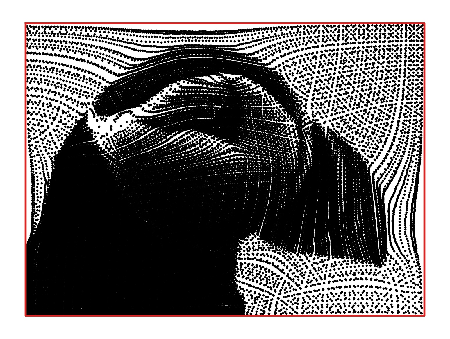
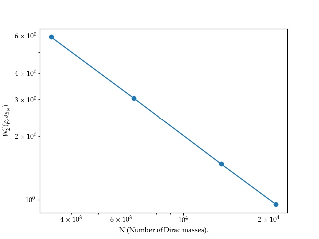
4 Numerical results
In this section, we report some experimental results in dimension .
Gray-scale image
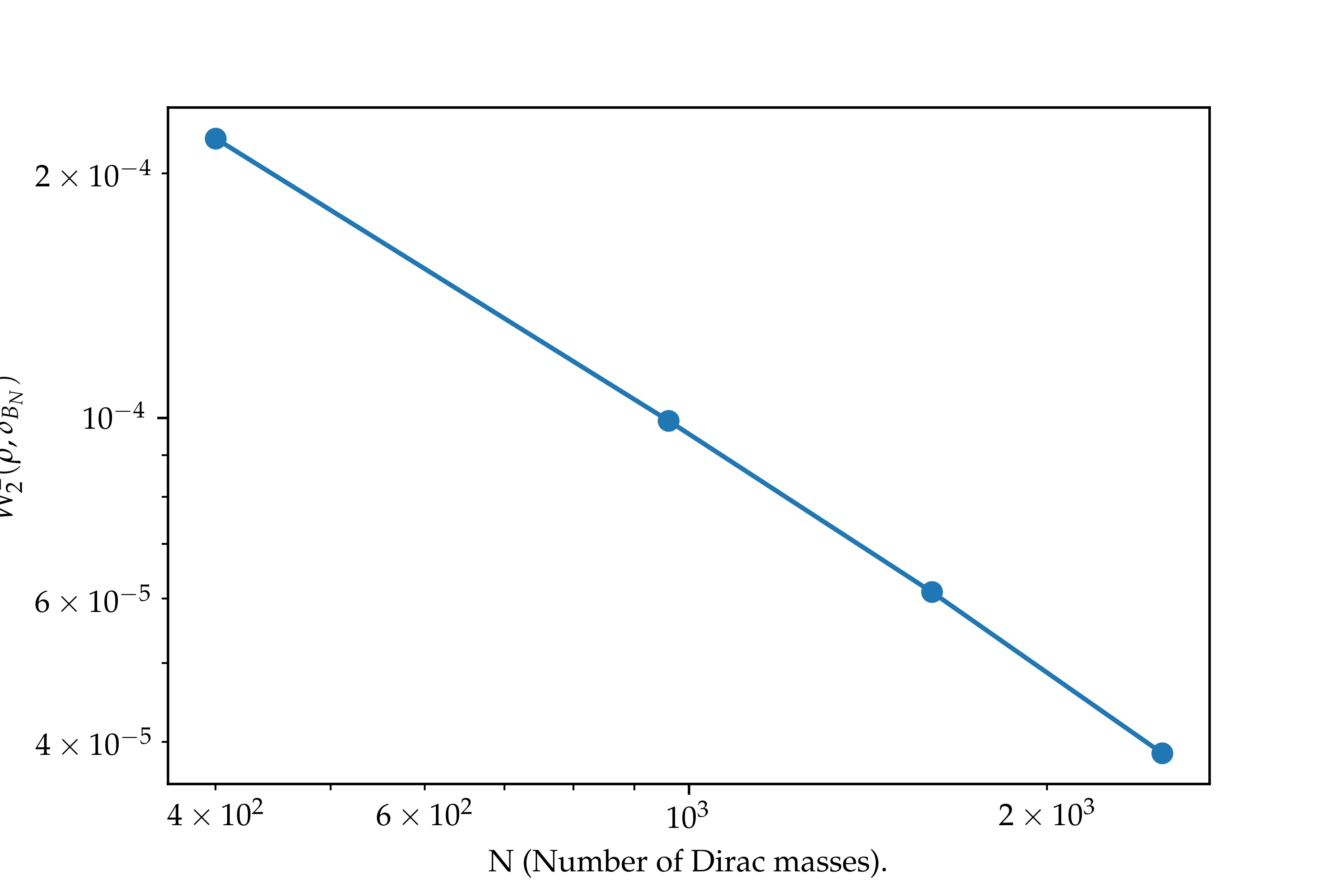
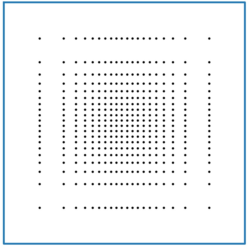
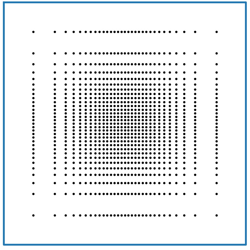
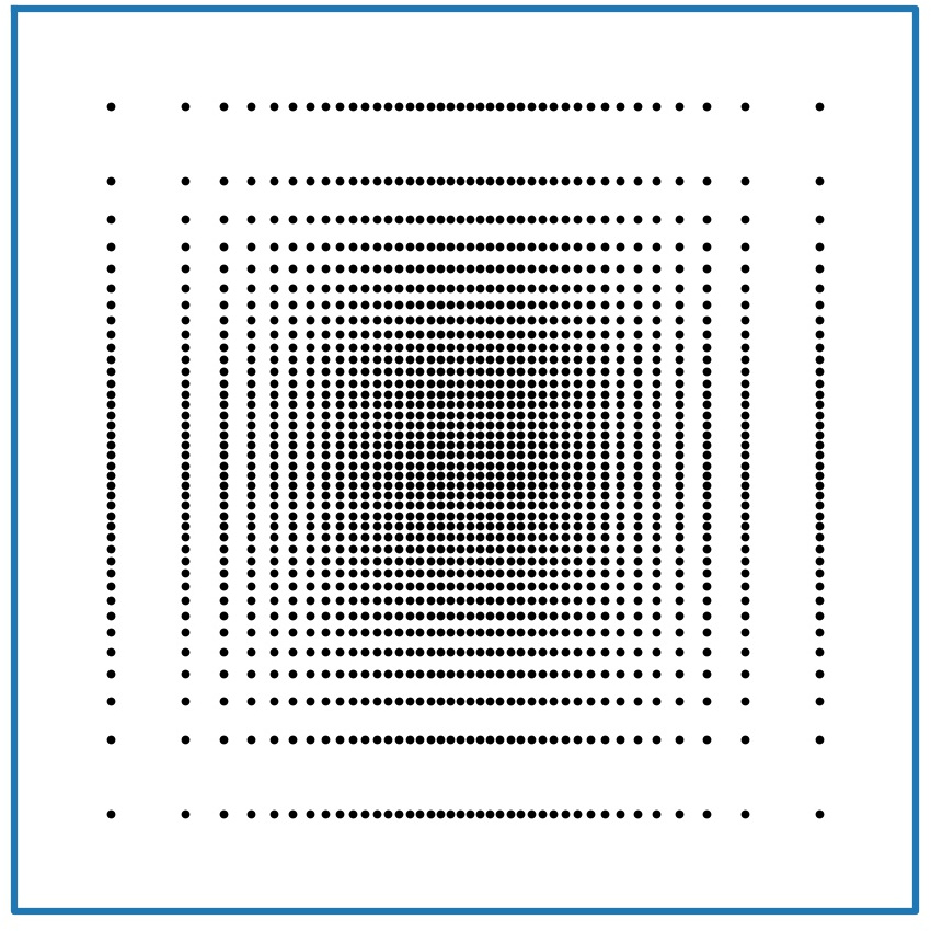
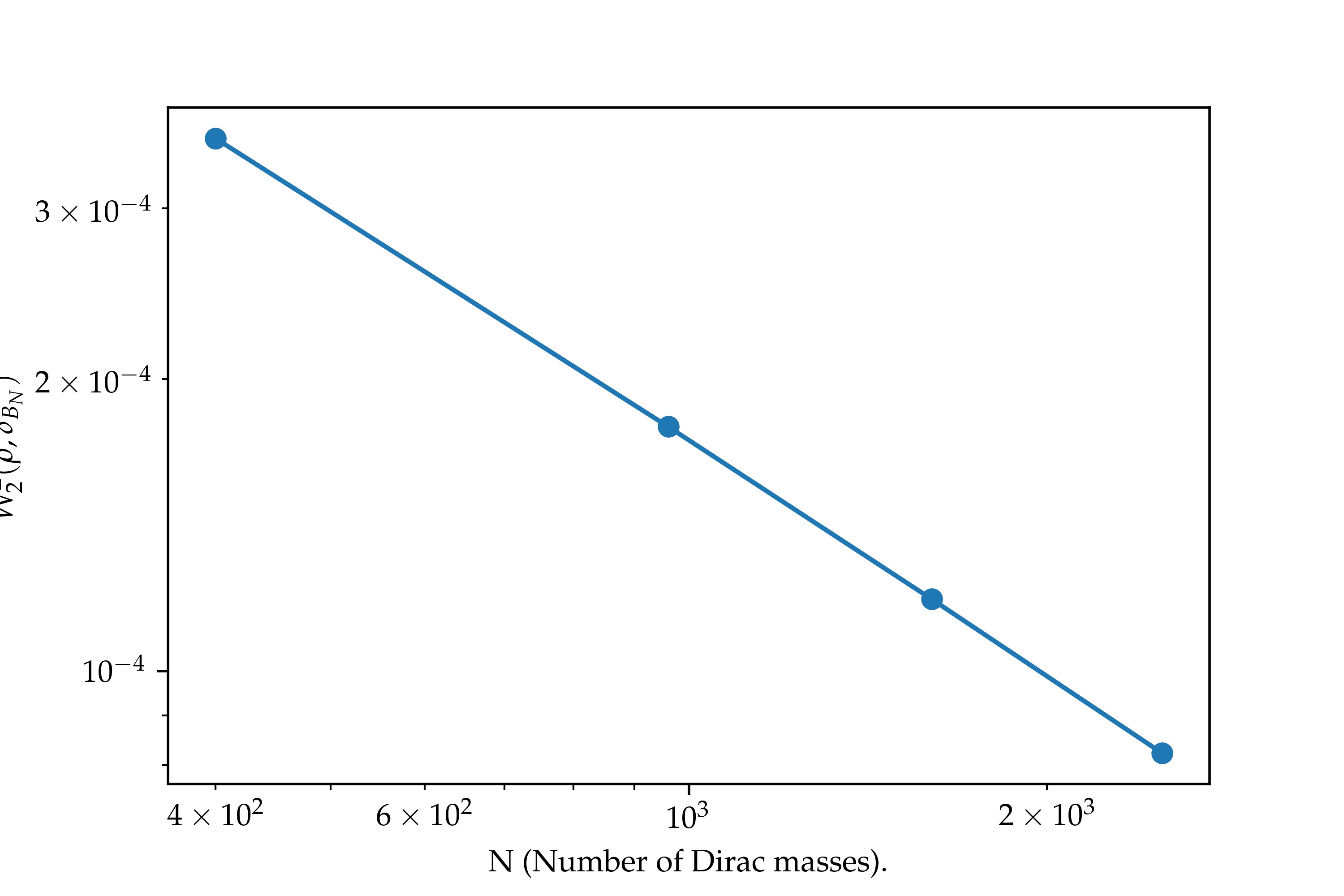
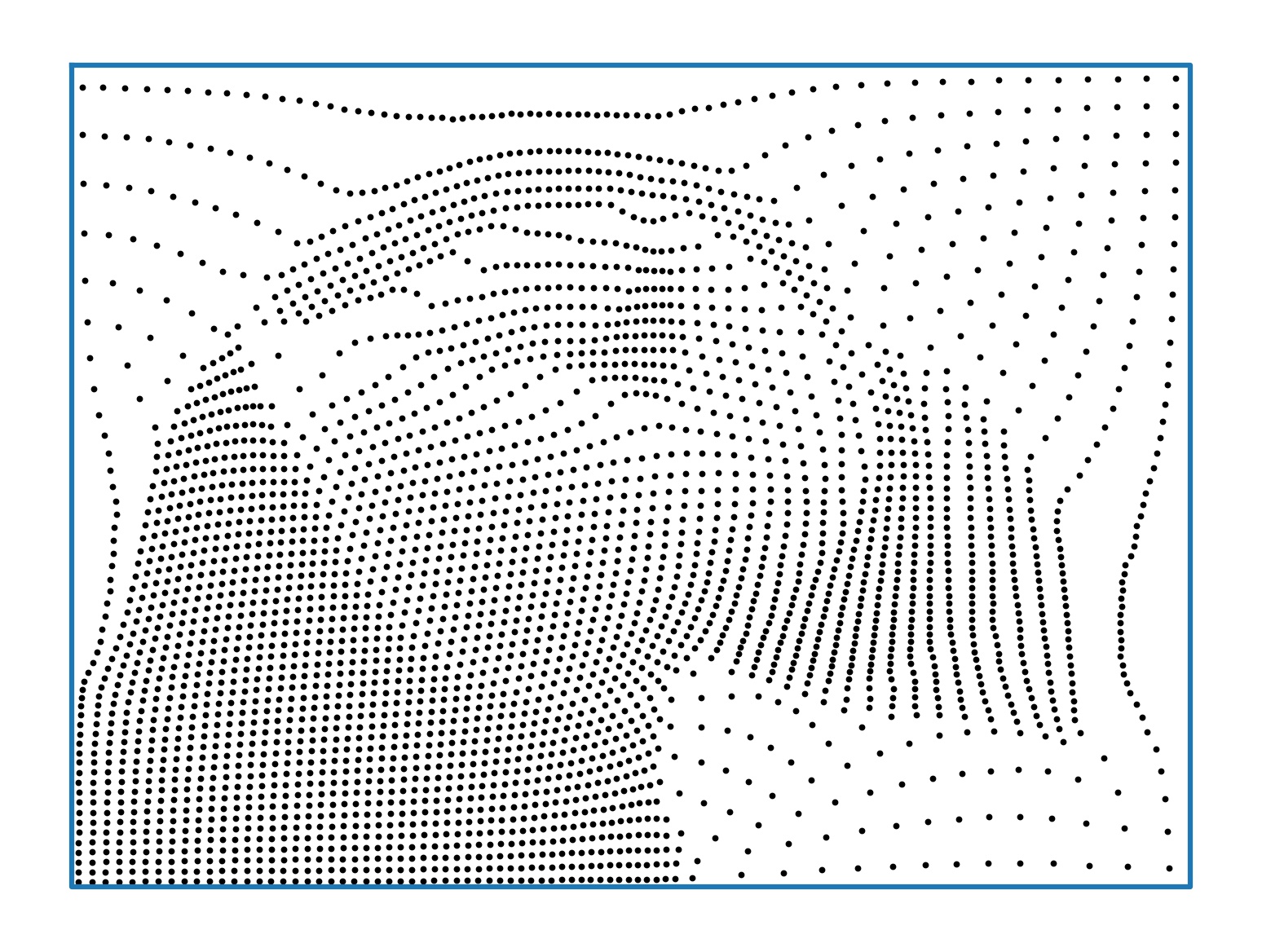
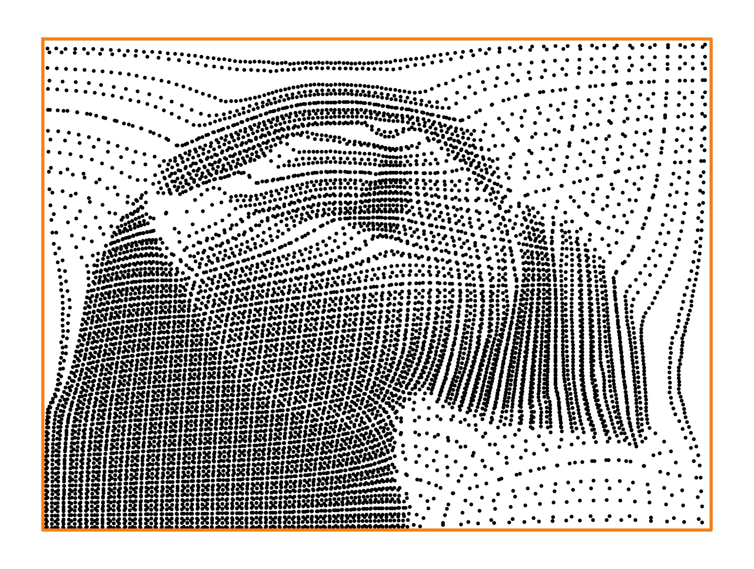
As we mentioned in the introduction, uniform optimal quantization allows to sparsely represent a (gray scale) image via points, clustered more closely in areas where the image is darker [4, 3]. On figure 3, we ploted the point clouds obtained after a single Lloyd step toward the density representing the image on the left (Puffin), starting from regular grids. The observed rate of convergence, , is coherent with the theoretical estimate of 1.
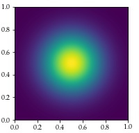
Gaussian density with small variance
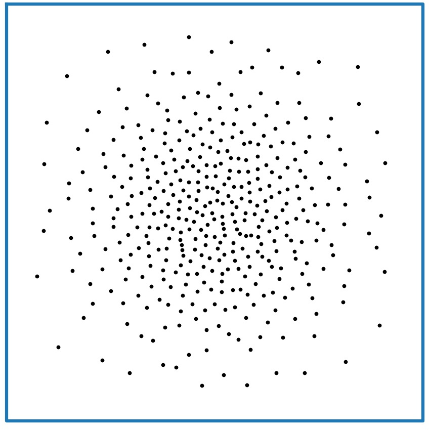
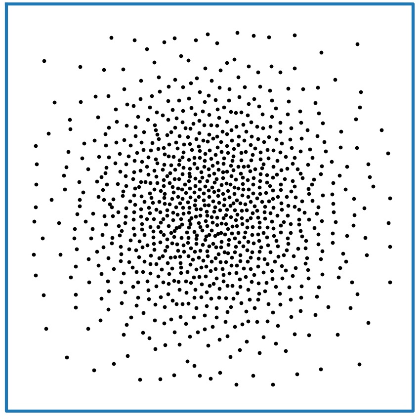
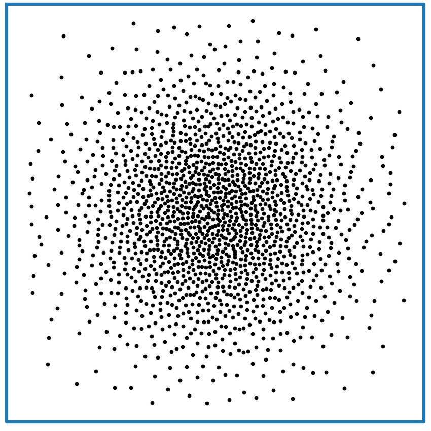
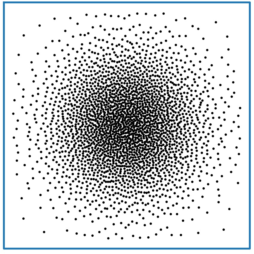
We now consider a toy model where we approximate a gaussian density truncated to the unit square , where is a normalization constant. On the left column of this figure, the initial point clouds are randomly distributed in . The three point clouds represented above are obtained after one step of Lloyd’s algorithm (14). The red curve displays in a log-log scale the mean values of over a hundred random point clouds, for . In this case, we observe a decrease rate with respect to the number of points, similar to the case of the gray scale picture.
However, an interesting phenomena occurs when the initial point cloud is aligned on a axis-aligned grid. The pictures in the right column of Fig. 2 where computed starting from such a grid with points. As in the randomly initialized case, we represented the values of in log-log scale. The corresponding discrete probability measure seems to converge to as , but with a much worse rate for these "low" values of : . In this specific setting, with a separable density and an axis-aligned grid , the power cells are rectangles and a single Lloyd step brings us to a critical point of . Thanks to this remark, it is possible to estimate the approximation error from the one-dimensional case. In fact, Appendix E shows that for any , there exists variances such that the approximation error is of order . On the other hand, for a fixed , the approximation error is of order , to be compared with the bound for general measures.
5 Discussion
We have studied the problem of minimizing the Wasserstein distance between a fixed probability measure and a uniform measure over points , parametrized by the position of the points . The main difficulty is the nonconvexity of the Wasserstein distance , which we tackled by means of a modified Polyak-Łojaciewicz inequality (20). One limitation of our work is that the terms replacing in the Polyak-Łojaciewicz inequality (20) does not match the theoretical bounds recalled in 1. Future work will concentrate on bridging that gap, but also on deriving consequences for the algorithmic resolution of Wasserstein regression problems starting with the case where is linear.
Acknowledgments and Disclosure of Funding
This work was supported by a grant from the French ANR (MAGA, ANR-16-CE40-0014).
References
- [1] Luigi Ambrosio, Nicola Gigli, and Giuseppe Savaré. Gradient flows: in metric spaces and in the space of probability measures. Springer Science & Business Media, 2008.
- [2] Martin Arjovsky, Soumith Chintala, and Léon Bottou. Wasserstein generative adversarial networks. In International conference on machine learning, pages 214–223. PMLR, 2017.
- [3] Michael Balzer, Thomas Schlömer, and Oliver Deussen. Capacity-constrained point distributions: a variant of lloyd’s method. ACM Transactions on Graphics (TOG), 28(3):1–8, 2009.
- [4] Fernando De Goes, Katherine Breeden, Victor Ostromoukhov, and Mathieu Desbrun. Blue noise through optimal transport. ACM Transactions on Graphics (TOG), 31(6):1–11, 2012.
- [5] Qiang Du, Maria Emelianenko, and Lili Ju. Convergence of the lloyd algorithm for computing centroidal voronoi tessellations. SIAM journal on numerical analysis, 44(1):102–119, 2006.
- [6] Bjorn Engquist, Brittany D Froese, and Yunan Yang. Optimal transport for seismic full waveform inversion. Communications in Mathematical Sciences, 14(8):2309–2330, 2016.
- [7] Jean Feydy, Benjamin Charlier, François-Xavier Vialard, and Gabriel Peyré. Optimal transport for diffeomorphic registration. In International Conference on Medical Image Computing and Computer-Assisted Intervention, pages 291–299. Springer, 2017.
- [8] Aude Genevay, Gabriel Peyré, and Marco Cuturi. Learning generative models with Sinkhorn divergences. In International Conference on Artificial Intelligence and Statistics, pages 1608–1617. PMLR, 2018.
- [9] Fernando de Goes, Pooran Memari, Patrick Mullen, and Mathieu Desbrun. Weighted triangulations for geometry processing. ACM Transactions on Graphics (TOG), 33(3):1–13, 2014.
- [10] Siegfried Graf and Harald Luschgy. Foundations of quantization for probability distributions. Springer, 2007.
- [11] Jun Kitagawa, Quentin Mérigot, and Boris Thibert. Convergence of a newton algorithm for semi-discrete optimal transport. Journal of the European Mathematical Society, 21(9):2603–2651, 2019.
- [12] Stuart Lloyd. Least squares quantization in pcm. IEEE transactions on information theory, 28(2):129–137, 1982.
- [13] Robert J McCann. A convexity principle for interacting gases. Advances in mathematics, 128(1):153–179, 1997.
- [14] Quentin Mérigot and Jean-Marie Mirebeau. Minimal geodesics along volume-preserving maps, through semidiscrete optimal transport. SIAM Journal on Numerical Analysis, 54(6):3465–3492, 2016.
- [15] Gilles Pagès. Introduction to vector quantization and its applications for numerics. ESAIM: proceedings and surveys, 48:29–79, 2015.
- [16] Gabriel Peyré, Marco Cuturi, et al. Computational optimal transport: With applications to data science. Foundations and Trends® in Machine Learning, 11(5-6):355–607, 2019.
- [17] Filippo Santambrogio. Absolute continuity and summability of transport densities: simpler proofs and new estimates. Calculus of variations and partial differential equations, 36(3):343–354, 2009.
- [18] Filippo Santambrogio. Optimal transport for applied mathematicians, volume 55. Springer, 2015.
- [19] Cédric Villani. Topics in optimal transportation. Number 58. American Mathematical Soc., 2003.
- [20] Cédric Villani. Optimal transport: old and new, volume 338. Springer Science & Business Media, 2008.
Appendix A Proof of 2
Given , one has for any ,
Summing these equalities over and remarking that the map defined by is an optimal transport map between and , we get
Thus, with , we have
This implies that the values of are decreasing in and, since they are bounded from below, that since . The sequence can be easily seen to be bounded, since is bounded, which implies a bound on the second moment of .
For fixed , since all atoms of have mass , this implies that all points belong to a same fixed compact ball. If itself is compactly supported, we can also prove that all points are contained in a compact subset of , which means obtaining a lower bound on the distances for arbitrary . This lower bound can be obtained in the following way: since is absolutely continuous it is uniformly integrable which means that for every there is such that for any set with Lebesgue measure we have . We claim that we have , where is such that is supported in a ball of radius . Indeed, it is enough to prove that every barycenter is at distance at least from each face of the convex polytope . Consider a face of such a polytope and suppose, by simplicity, that it lies on the hyperplane with the cell contained in . Let be such that . Then since the diameter of is smaller than , the Lebesgue measure of is bounded by , which provides because of the definition of . Since at least half of the mass (according to ) of the cell is above the level the -coordinate of the barycenter is at least . This shows that the barycenter lies at distance at least from each of its faces.
As a consequence, the iterations of the Lloyd algorithm lie in a compact subset of , on which is . This implies that any limit point must be a critical point.
We do not discuss here whether the whole sequence converges or not, which seems to be a delicate matter even for fixed . It is anyway possible to prove (but we do not develop the details here) that the set of limit points is a closed connected subet of with empty interior, composed of critical points of all lying on a same level set of .
Appendix B Proof of 5
Given , we denote
We call points such that -isolated, and points such that -connected.
Lemma 1.
Let be independent, -valued, random variables. Then, there is a constant such that
Proof.
This lemma is a consequence of McDiarmid’s inequality. To apply this inequality, we need evaluate the amplitude of variation of the function along changes of one of the points . Denote the maximum cardinal of a subset of the ball such that the distance between any distinct points in is at least . By a scaling argument, one can check that does not, in fact, depend on . To evaluate
we first note that at most points may become -isolated when removing . To prove this, we remark that if a point becomes -isolated when is removed, this means that and for all . The number of such is bounded by . Symmetrically, there may be at most points becoming -connected under addition of . Finally, the point itself may change status from -isolated to -connected. To summarize, we obtain that with ,
The conclusion then directly follows from McDiarmid’s inequality. ∎
Lemma 2.
Let be a probability density and let be i.i.d. random variables with distribution . Then,
Proof.
The probability that a point belongs to the ball for some can be bounded from above by , where is the volume of the -dimensional unit ball. Thus, the probability that is -isolated is larger than
We conclude by noting that
Proof of 5.
We apply the previous 2 with and . The expectation of is lower bounded by:
for large , since . By 1, for any ,
for constants depending only on and . We choose , so that is of the same order as since .Thus, for a slightly different ,
Now, for such that
3 yields:
and such a disposition happens with probability at least
Appendix C Proof of 6
Appendix D Proof of 7
Lemma 3.
Let for some . Then, the iterates of (13) satisfy for every , and for every
| (23) |
Proof.
We consider the distance between two trajectories after iterations: Assuming that , the convexity of the norm immediately gives us:
where we denoted the barycenter of the th Power cell in the tesselation associated with the point cloud . Since each barycenter lies in its corresponding Power cell, the scalar product is non-negative: Indeed, for any ,
Summing this inequality with the same inequality with the roles of and reversed, we obtain:
thus giving us the geometric inequality . Since was chosen in , this yields and inequality 23. ∎
Lemma 4.
For any
| (24) |
where we denote and .
Proof.
This is obtained in a very similar fashion as 3. For any , the semi-concavity of yields the inequality:
with in accordance with the previous proof.
Proof of 7.
To conclude, we simply make (order 1) expansions of the terms in 24. The definition of in 7, although convoluted, was made so that both terms in the right-hand side of this inequality, and have the same asymptotic decay to (as ): With the notations of the previous proposition, we have for fixed :
| (25) |
We make use here of the notation from Section 3:
to clear this expression a bit, and, because of the assumption , we may write:
as well as , and substituting ,
Appendix E Case of a low variance Gaussian in Section 4
Here, we consider the probability measure obtained by truncating and renormalizing a centered normal distribution with variance to the segment . We first show that for any and , we can find a small such that the Wasserstein distance beween and its best -points approximation of is at least .
Proposition 8.
For any , consider the truncated centered Gaussian density, where is taken so that has unit mass. Then, for every , there exists a constant and a sequence of variances such that
From the proof, one can see that the dependence of on is logarithmic.
Proof.
We denote the density of the centered Gaussian distribution and its cumulative distribution function, so that
| (26) |
Note that, whenever , we have . We denote by the cumulative distribution function of . Given any point cloud such that , the Power cells is simply the segment
Since these segments do not depend on , we will denote them . Finally, defining as the barycenter of the th power cell and , we have
| (27) | ||||
where we used that attains its minimum at to get the first inequality. We now wish to provide an approximation for , . We first note, using Taylor’s formula, that we have
for some . But,
and we see that
Therefore, if we denote the second-order error in the above formula, i.e. , the size of the first Power cell is of order:
We will choose depending on in order for the first term in the left-hand side to dominate the second one:
| (28) |
In this way, we have
| (29) |
The following corollary, whose proof can just be obtained by adapting the above proof to a simple multi-dimensional setting where measures and cells “factorize” according to the components, confirms the facts observed in the numerical section (Section 4), and the sharpness of our result (Remark 4).
Corollary 9.
Fix . Given any , consider an axis-aligned discrete grid of the form in , with , where each is a subset of with cardinal . Finally, define as in 8 Then we have
where the constant is independent of .