Non-convex non-local flows for saliency detection
Abstract
We propose and numerically solve a new variational model for automatic saliency detection in digital images. Using a non-local framework we consider a family of edge preserving functions combined with a new quadratic saliency detection term. Such term defines a constrained bilateral obstacle problem for image classification driven by -Laplacian operators, including the so-called hyper-Laplacian case (). The related non-convex non-local reactive flows are then considered and applied for glioblastoma segmentation in magnetic resonance fluid-attenuated inversion recovery (MRI-Flair) images. A fast convolutional kernel based approximated solution is computed. The numerical experiments show how the non-convexity related to the hyper-Laplacian operators provides monotonically better results in terms of the standard metrics.
Index terms— Variational Methods, Non-local Image Processing, Automatic Saliency Detection, MRI-Flair Glioblastoma Segmentation.
1 Introduction
Image processing by variational methods is an established field in applied mathematics and computer vision which aims to model typical low and mid level image reconstruction and restoration processes such as denoising, deconvolution, impainting, segmentation and registration of digital degraded images. Since the mathematical approach of Tikhonov and Arsenin on ill-posed inverse problems [3] and the applied work of Rudin, Osher and Fatemi [21] through their celebrated ROF model, there have been a standing effort to deal with new image processing tasks through variational methods. Currently there is a growing interest in image processing and computer vision applications for visual saliency models, able to focus on perceptually relevant information within digital images.
Semantic segmentation, object detection, object proposals, image clustering, retrieval and cognitive saliency applications, such as image captioning and high-level image understanding, are just a few examples of saliency based models. Saliency is also of interest as a means for improving computational efficiency and for increasing robustness in clustering and thresholding.
Despite of the lack of a general consensus on a proper mathematical definition of saliency, it has a clear biologically perceptive meaning: it models the mechanism of human attention, that is, of finding relevant objects within an image.
Recently, there has been a burst of research on saliency due to its wide application in leading medical disciplines such as neuroscience and cardiology. In fact, when considering medical images like those acquired in magnetic resonance imaging (MRI) or positron emission tomography (PET), the automatic obtention of saliency maps is useful for pathology detection, disease classification [22], location and segmentation of brain strokes, gliomas, myocardium detection for PET images, tumors quantification in FLAIR MRI [23], etc.
The role of saliency in models is application dependent, and several different techniques and approaches have been introduced to construct saliency maps. They vary from low dimensional manifold features minimization [27] to non-local sparse minimization [25], graphs techniques [9], partial differential equations (PDE) [12], superpixel [14], learning [13], or neural networks based approaches [4] (MIT-Benchmark).
With the aim to explore the applications and algorithms of non-smooth, non-local, non-convex optimization of saliency models, we present in this article a new variational model applied to Fluid Attenuated Inversion Recovery (FLAIR) MR images for accurate location of tumor and edema.
Models for saliency detection try to transform a given image, , defined in the pixel domain, , into a constant-wise image, , whose level sets correspond to salient regions of the original image. They are usually formulated through the inter-relation among three energies: fidelity, regularization, and saliency, being the latter the mechanism promoting the classification of pixels into two or more classes. There is a general agreement in considering the fidelity term as determined by the norm, that is
so that departure from the original state is penalized in the minimization procedure.
For regularization, an edge preserving energy should be preferred. The use of the Total Variation energy,
defined on the space of Bounded Variation functions has been ubiquitous since its introduction as an edge preserving restoration model [21]. Indeed, the Total Variation energy allows discontinuous functions to be solutions of the corresponding minimization problem, with discontinuities representing edges. This is in contrast to Sobolev norms, which enforce continuity across level lines and thus introduce image blurring. Only recently, the non-local version of the Total Variation energy and, in general, of the energy associated to the -Laplacian, for , has been considered in restoration modeling. In saliency modeling, only the range seems to have been treated [12]. One of the main advantages of introducing these non-local energies is the lack of the hard regularizing effect influencing their local counterparts.
For the saliency term, a phase-transition Ginzburg-Landau model consisting in a double-well absorption-reaction term is often found in the literature [8]. The resulting energy is a functional of the type
whose minimization drives the solution towards the discrete set of values , facilitating in this way the labeling process. However, due to the vanishing slope of at , the resulting algorithm has a slow convergence to the minimizer.
In this article, we introduce new regularizing and saliency terms that enhance the convergence of the classification algorithm while keeping a good quality compromise. As regularizing term, we propose the non-local energy associated to the -Laplacian for any , see Eq. (3). Although there is a lack of a sound mathematical theory for the concave range , computational evidence of the ability of these energies to produce sparse gradient solutions has been shown [11]. In any case, our analysis also includes the energies arising for , enjoying a well established mathematical theory.
With respect to the saliency term, we consider the combination of two effects. One is captured by the concave energy
with constant, which fastly drives the minimization procedure so that . To counteract this tendency and remain in the meaningful interval , being the saliency labels employed in this article, we introduce an obstacle which penalizes the minimization when the solution lies outside . The modeling of such obstacle is given in terms of the indicator function
and the resulting saliency term is then defined as a weighted sum of the operators and .
Finally, the Euler-Lagrange equation for the addition of these three energies leads to a formulation of a multi-valued non-local reaction-diffusion problem which is later rendered to a single-valued equation by means of the Yosida’s approximants. The introduction of a gradient descent and the discretization of the corresponding evolution equation are the final tools we use to produce our saliency detection algorithm.
The main contributions contained in this paper may be summarized as follows.
-
•
The non-local -Laplacian convex model proposed in [12], valid for , is extended to include the range . Notably, the non-differentiable non-convex fluxes related to the range are investigated.
-
•
An absorption-reaction term of convex-concave energy nature is considered for fast saliency detection. In absence of a limiting mechanism, the reactive part could drive the solution to take values outside the image range . Thus, a penalty term is introduced to keep the solution within such range.
-
•
The resulting multivalued constrained variational formulation is approximated and shown to be stable.
-
•
A fast algorithm overcoming the computational drawbacks of non-local methods is presented.
-
•
A 3D generalization of the model is considered providing promising results specially valuable in medical image processing and tumor detection.
The paper is organized as follows. In Section 2, we introduce the variational mathematical framework of our models. Starting with the local equations as guide for the modelling exercise, we focus on the non-local diffusive terms, explicited in the form of -Laplacian, for and extend it to the range through a differentiable family of fluxes to cover the resulting non-local non-convex hyper-Laplacian operators. Then, we introduce a multi-valued concave saliency detection term which defines an obstacle problem for the non-local diffusion models. In Section 3 we deduce the corresponding Euler-Lagrange equations. A gradient descent approximation is finally used to solve the elliptic non-local problems until stabilization of the associated evolution problems. In Section 4, we give the discretization schemes used for the actual computation of the solutions of the non-local diffusion problems. In Section 5 a simplified computational approach is described in order to reduce the time execution with a view to a massive implementation on the proposed data-set. Section 6 contains the numerical experiments on the proposed model and present the simulations performed on FLAIR sequences of MR images obtained from the BRATS2015 dataset [16]. Finally, in Section 7, we give our conclusions.
2 Variational framework
2.1 Local -Laplacian
Variational methods have shown to be effective to model general low level computer vision processing tasks such as denoising, restoration, registration, deblurring, segmentation or super-resolution among others. A fundamental example is given by the minimization of the energy functional
| (1) |
where is a constant, and are the regularization and the fidelity terms, respectively, given by
is the set of pixels, is the image to be processed, and belongs to a space of functions for which the minimization problem admits a solution. The idea behind this minimization problem is: given a non-smooth (e.g. noisy) image, , obtain another image which is close to the original (fidelity term) but regular (bounded gradient in ). The parameter is a weight balancing the respective importance of the two terms in the functional.
When first order necessary optimality conditions are imposed on the energy functional, a PDE (the Euler-Lagrange equation) arises. In our example,
| (2) |
The divergence term in this equation is termed as -Laplacian, and its properties have been extensively studied in the last decades for the range of exponents . For , the energy is convex and differentiable, and the solution to the minimization problem belongs to the Sobolev space , implying that can not have discontinuities across level lines. Therefore, the solution, , is smooth even if the original image, , has steep discontinuities (edges). This effect is known as blurring: the edges of the resulting image are diffused.
In the case , the energy term is convex but not differentiable. The solution of the related minimization problem (the Gaussian Denoising model [21, 5] or the Rician Denoising model [15]) belong to the space of functions of Bounded Variation, , among which the constant-wise functions play an important role in image processing tasks [1]. Thus, in this case, the edges of are preserved in the solution, , because a function of bounded variation may have discontinuities across surface levels.
In this article, we are specially interested in the range , for which the energy is neither convex nor differentiable, and it only generates a quasi-norm on the corresponding space. In this parameter range the problem lacks of a sound mathematical theory, although some progress is being carried on [10]. Despite the difficulties for the mathematical analysis, there is numerical evidence on interesting properties arising from this model. In particular, the non-convexity forces the gradient to be sparse in so far it minimizes the number of jumps in the image domain. Actually, only sharp jumps are preserved, looking the resulting image like a cartoon piecewise constant image.
2.2 Nonlocal -Laplacian
While for the use of the local -Laplacian energy is not specially relevant in image processing due to its regularizing effect on solutions which produces over-smoothing of the spatial structures, for its non-local version the initial data and the final solution belong to the same functional space, that is, no global regularization takes place. See [2], where a thorough study on non-local diffusion evolution problems, including existence and uniqueness theory, may be found.
The non-local analogous to the energy , for , is
| (3) |
where is a continuous non-negative radial function with and . The Fréchet differential of is
Thus, the Euler-Lagrange equation for the minimization problem (1) when is replaced by is
| (4) |
For , the Euler-Lagrange equation (4) does not have a precise meaning due to the singularities that may arise when the denominator vanishes. To overcome this situation, we approximate the non-differentiable energy functional by
for , where
Observe that the corresponding minimization problem is now well-posed due to the differentiability of . Therefore, a solution may be calculated solving the associated Euler-Lagrange equations. However, for , the solution is in general just a local minimum, due to the lack of convexity. Of course, the same plan may be followed for the local diffusion equation (2).
2.3 Saliency modeling
The previous section highlighted the connections between local and non-local formulations. From now on, we focus on the non-local diffusion model, being the model deduction similar for the case of local diffusion.
For saliency detection and classification, an additional term is added to the energy functional (1) or to its non-local or regularized variants. The general idea is pushing the values of towards the discrete set of extremal image values , determining the labels we impose for saliency detection: for foreground, and for background.
To model this behavior we propose a two-terms based energy, where the first causes a reaction extremizing the values of the solution and the second accounts for the problem constraints (). The first term is given by the energy
for some constant . The corresponding energy minimization drives the solution away from the zero maximum value, attained at , and it would be unbounded () if no box constraint were assumed.
However, under the box constraint, the global minimum of in is attained at the boundary of this interval, that is, at the labels of saliency identification. Therefore, together with the box constraint promote the detection of salient regions of interest (foreground) separated by regions with no relevant information (background).
The box constraint is accomplished through the indicator functional of the interval , defined as
Observe that since is convex and closed, the functional is convex and lower semi-continuous, and that its sub-differential is the maximal monotone graph of , given by
The saliency term we propose is therefore the sum of the fast saliency promotion, , and of the range limiting mechanism, , i.e.
3 The model. Approximation and estability
Gathering the fidelity, the regularizing and the saliency energies, we define a bilateral constrained obstacle problem associated to the following energy
| (5) |
where is a parameter modulating the relationship between regularization and saliency promotion. Observe that there is no use in multiplying by the constant , so we omit it for clarity.
The Euler-Lagrange equation corresponding to (5) together with the use of a gradient descent method leads to the consideration of non-local multi-valued evolution problems.
Multi-valued Problems
Let , , and be real fixed positive parameters. Let moreover be an (essentially) bounded function. For some given , find solving the approximating smooth (in fact differentiable) multivalued problems
| (6) |
which model non-linear non-local non-convex reactive flows that we shall consider in the range .
For the sake of presentation, we have introduced the following notation in (6): we rewrote the Fréchet differential of as , with
| (7) |
and defined the non-local hyper-Laplacian () and -Laplacian () diffusion operators
with differential kernels
| (8) |
Notice that, while for the local diffusion problem we must explicitly impose the homogeneous Neumann boundary conditions, which are the most common boundary conditions for image processing tasks, for the non-local diffusion problem this is no longer necessary since these conditions are implicitly imposed by the non-local diffusion operator [2].
3.1 Yosida’s approximants
Introducing the maximal monotone graphs given by
we may express the subdifferential of as . The Yosida’s approximants of and are then
for , allowing us to approximate the multi-valued formulation (6) by single-valued equations in which and are replaced by and . This is, by the evolution PDE
| (9) |
Assume that a solution, , of (9) with initial data does exist, and consider the characteristic function of a set , defined as if and otherwise. Introducing the sets
for , we may express the Yosida’s approximants appearing in (9) as
with, for , . Then, we rewrite (9) as a family of approximating problems .
Approximating Single-Valued Problems
Notice that and , where we used the notation , , so that .
The following result generalizes to the non-local framework the results of [17], establishing that the solution of (10) is such that the subset of where may be done arbitrarily small by decreasing . Thus, in the limit the solution does not overpass the obstacles and .
Theorem 1.
Let and assume that the parameters are positive. If is the corresponding solution of (10), then
for some constant independent of .
Proof. Multiplying (10) by and integrating in , we obtain
| (11) |
where we used . Since is an odd function, the following integration by parts formula holds
Thus, in noting that is non-increasing as a function of , we deduce
and therefore, see (8),
| (12) |
Using (12) and the Schwarz’s inequality in (11) we get,
| (13) |
Getting rid of the term , we apply Gronwall’s inequality to the resulting inequality to obtain
with . Using this estimate in (13) yields
with . Finally, integrating in and using that , we obtain
| (14) |
for some constant independent of . To finish the proof we must show that also
Since, once we multiply (10) by and integrate in , the arguments are similar to those employed to get estimate (14), we omit the proof.
4 Discretization of the limit problem
In the previous section we have shown that solutions of the multivalued problem (6) may be approximated by the introduction of Yosida’s approximants, leading to the single-valued problems in (10) that depend on the Yosida’s approximation parameter . We also proved that in the limit the corresponding solutions lie in the relevant range of values for image processing tasks, this is, in the interval .
In this section we provide a fully discrete algorithm to numerically approximate the limit solution of (10) when . First, we introduce a time semi-implicit Euler discretization of the evolution equation in (10), that we show to retain the stability property of its continuous counterpart, stated in Theorem 1.
The resulting space dependent PDE is discretized by finite differences. Since the problem is nonlinear and, in addition, we want to pass to the limit , we introduce an iterative algorithm which renders the problem to a linear form and, at the same time, replaces the fixed parameter by a decreasing sequence .
4.1 Time discretization
For the time discretization, let , , and consider the decomposition , with . We denote by to and by to , for . Then, we consider a time discretization of (10) in which all the terms are implicit but the diffusion term, which is semi-implicit. The resulting time semi-discretization iterative scheme is:
Iterative Problems
Given , , , a.e. in set and for find such that
| (15) |
where, for , we define
| (16) |
That is, only the modulus part of the diffusion term is evaluated in the previous time step.
Equation (15) is still nonlinear (in fact piece-wise linear) due to the Yosida’s approximants of the penalty term. In addition, its solution depends on the fixed parameter that, in view of Theorem 1, we wish to make arbitrarily small, so that the corresponding solution values are effectively constrained to the set . To do this, we consider the following iterative algorithm to approximate the -dependent solution, , of (15) when .
Iterative Approximating Problems
Let , and be as before. Let and be given. For , set . Then, for , define and, until convergence, solve the following problem: find such that
| (17) |
where for , being
We use the stopping criteria
| (18) |
for values of chosen empirically and, when satisfied, we set .
4.2 Space discretization
For the space discretization, we consider the usual uniform mesh associated to image pixels contained in a rectangular domain, , with mesh step size normalized to one. We denote by a generic node of the mesh, with , and by a generic function evaluated at
To discretize the non-local diffusion term in space, we assume that is a constant-wise interpolator, and to fix ideas, we use the common choice of spatial kernel used in bilateral theory filtering [24], that is, the Gaussian kernel
being a normalizing constant such that . Assuming that the discretized version of is compactly supported in , with the support contained in the box , we use the zero order approximation (16)
where and .
The values of the characteristic functions of the set are the last terms of (17) that we must spatially discretize. This is done by simply examining whether or not, for , and similarly for .
The full discretization of (17) takes the form of the following linear algebraic problem: For , let . For , set . Then, for until convergence, solve the following problem: find such that
| (19) |
The convergence of the algorithm is checked at each -step according to the spatial discretization of the stopping criterium (18), that is
When the stopping criterium is satisfied, we set and advance a new time step, until is reached.
5 A simplified computational approach
In the previous sections we have deduced, through a series of approximations, a discrete algorithm to compute approximated solutions of the obstacle problem in (6). We have shown that our scheme is stable with respect to the approximating parameter , producing solutions of problems that, in the limit , lie effectively in the image value range , apart from producing the required edge preserving saliency detection on images.
In this section, by introducing some hard nonlinearities (truncations) to replace one of the iterative loops of (19), we provide a simplified algorithm for solving a problem closely related to (6). In addition, we use an approximation technique, based on the discretization of the image range, to compute the non-local diffusion term. These modifications allow for a fast computation of what we demonstrate to be fair approximations to the solutions of the original problem (6).
Considering the time discrete problem (15), we introduce two changes which greatly alleviate the computational burden:
-
1.
Compute the non-local diffusion term fully explicitly, and
-
2.
Replace the obstacle term by a hard truncation.
Thus, we replace problem in (15) by the following which can be deduced from problem in (6) using the two above strategies.
Explicit Truncated Problems
Given , and for , find such that
| (20) |
followed by a truncation of within the range . Observe that, as remarked in [18], the explicit Euler scheme is well suited for non-local diffusion since it does not need a restrictive stability constraint for the time step, as it happens for the corresponding local diffusion. This is related to the lack of regularizing effect in non-local problems. Spatial discretization of (20) leads to the following algorithm which we shall refer as the patch based scheme:
Set . For , and for , compute
| (21) |
and truncate
We shall show that there are very small differences between the solutions of the explicit truncated problem and the solutions of the problems for sufficiently small. Nevertheless, the numerical scheme is greatly improved and much more efficient because costly iteration in -loop is avoid as it can be seen in section (6). We finally describe the efficient approach of [26] (see also [7], and and [6] for a related approach) that we use for computing the sum in (21), corresponding to the non-local diffusion term, by discretizing also the range of image values. Let be a quantization partition, with , where is the number of quantization levels. Let be a quantized function, that is, taking values on . For each , we introduce the discrete convolution operator
| (22) |
where we recall that . We then have
Notice that, for any taking values in , the computation of each may be carried out in parallel by means of fast convolution algorithms, e.g. the fast Fourier transform.
It is possible that, after a time iteration, a quantized iterand leads to values of not contained in the quantized partition , implying that the new operators should be computed in a new quantization partition, say . Since, for small time step, we expect and to be close to each other, we overcome this inconvenient by rounding to the closest value of the initial quantization vector, , so that this vector remains fixed.
The final simplified algorithm which we call the kernel based scheme is then:
Set . For , and for each , perform the following steps:
-
•
Step 1. If then using (22)
(23) -
•
Step 2. , where .
6 Numerical experiments
In this section we describe the experiments that support our conclusions. First, we compare the use of hard truncation (in the fully explicit numerical scheme (20)) with the iterative scheme () when the Yosida’s Approximants are used to solve the discrete problem (17). As a second test, the proposed kernel based approach in (23) is compared with the patch based scheme in (21). As an application of the above schemes, we test our approach over the BRATS2015 dataset [16]. Finally, we show that our model can be generalized presenting some preliminary results which extend our variational non-local saliency model to 3D volumes.
6.1 Experiment 1: Comparison between limit approximation and truncation
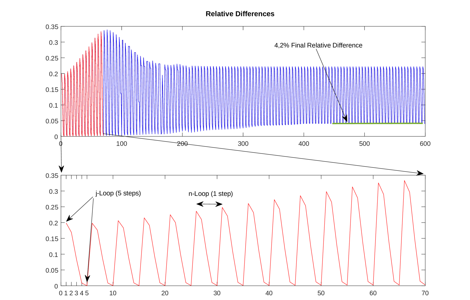
In this experiment we show the differences between the limit approximation described in section 4 and the proposed truncation alternative. We recall that the purpose of such hard truncation is to get rid of the -loop in the numerical resolution, boosting the computation efficiency. In practice, instead of using the stopping criteria (18), is sufficient (and more efficient) to fix a small number of iterations which results into 5 in the -loop starting with and setting . We found in our experiments that this is enough in order to ensure that the final output of the approximating scheme (17) is very close to the solution of (21).
Each -step consists of solving the equation (17) which is carried out through a conjugate gradient descent algorithm. This is an inner loop for each -step which increases substantially the global time execution of the algorithm. In order to show that the hard truncation is a good strategy to get rid of the -loop we compute the relative differences between each -step image () and the truncated version () of the -step solution.
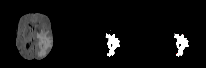
At each step of the -loop, the relative difference from the final truncated version is reduced. Figure 1 depicts the qualitative difference of using truncation. For all the subjects we tested the results clearly show that the same saliency (tumor) region is detected in both images. The differences, barely visibles, are colored in red. Indeed only few pixels differ from the assumed correct computation through the -convergence, which justifies the use of the hard truncation.
6.2 Experiment 2: Kernel based approach
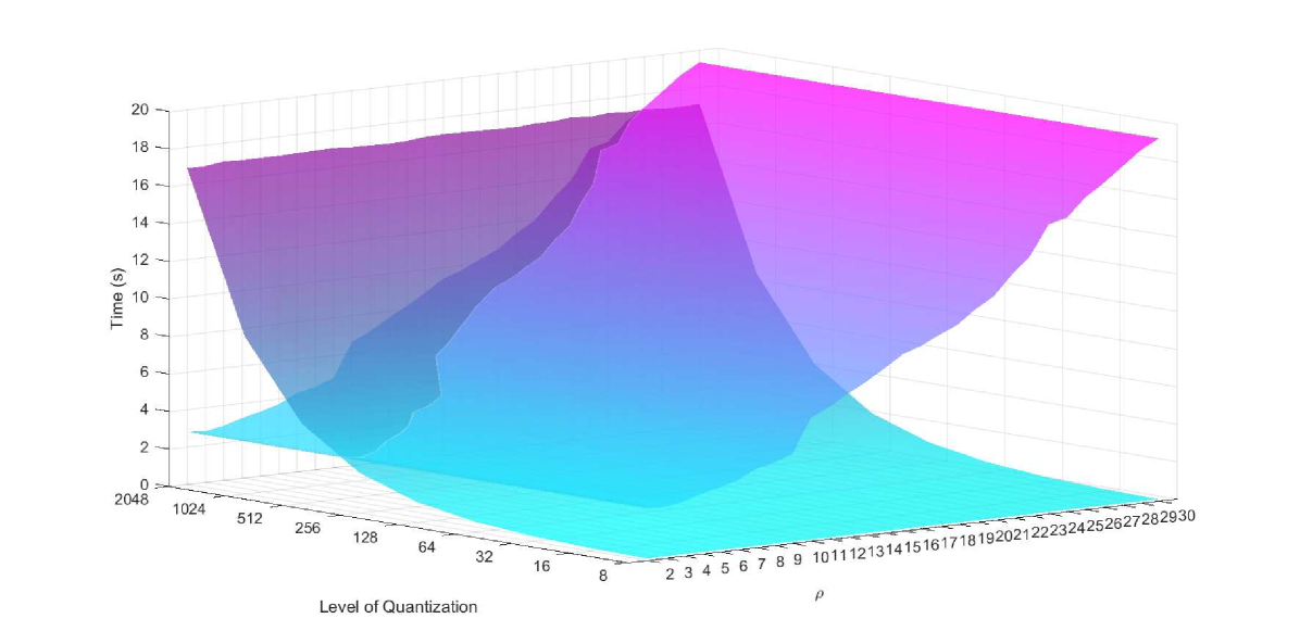
In this experiment we compare the time execution between patch based numerical resolution and the proposed kernel approach based on [26]. Taking advantage of the fact that convolutions can be fast computed in Fourier domain, we use a GPU implementation to carry out these experiments. In both cases we fix the same hyper-parameters and perform a sweep where is the kernel radio and are the quantization levels. The tests are performed over 4 brains (2 slices per brain) and results are averaged.
Notice that in a classical patch based approach no quantization is required and the time execution will grow up only with the size of the considered region (). On the contrary, a kernel based resolution remains robust to different kernel sizes while the time execution relays mainly in the number of quantization levels as it can be seen in figure 3. This justifies the use of the kernel based method whereas it allows to use bigger kernels so properly modelling the non-local diffusion term.
6.3 Experiment 3: MRI Dataset
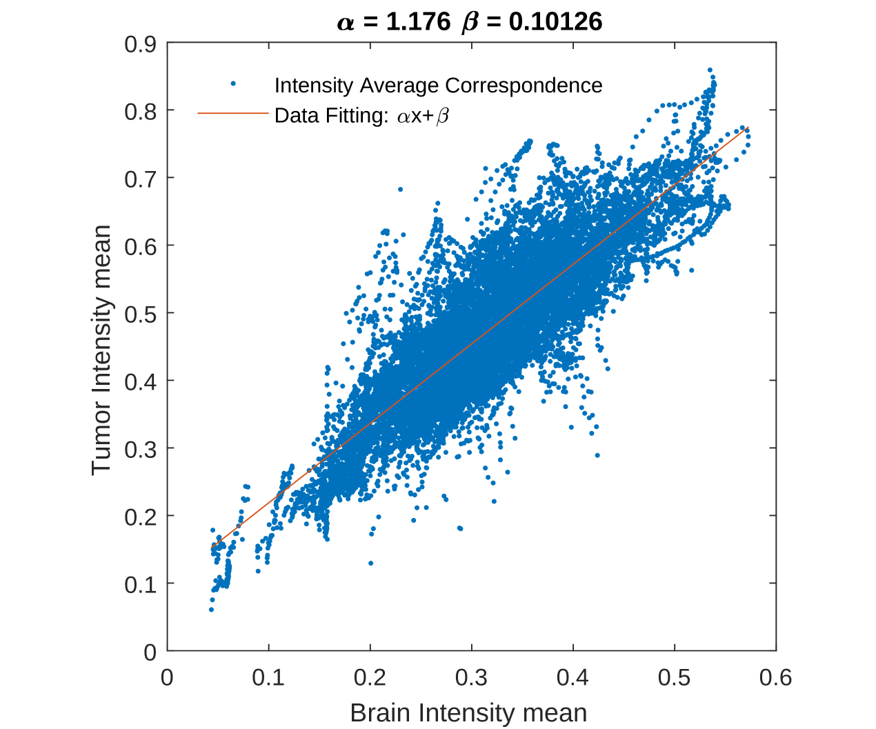
We then apply our above findings testing the whole BRATS2015 dataset [16]. In order to highlight the importance of the proposed non-local non-convex hyper-Laplacian operators we shall consider the behavior of the model when only the -parameter is modified. For such purpose we need to introduce an automated rule for the -parameter estimation to avoid a manual tuning of the model for each image of the dataset. This will result in a sub-optimal performance of the model in terms of accuracy. Nevertheless, it will provide us a good baseline of how good is our proposed model. Observing that acts as threshold between classes (background and foreground), we seek a rule to determine such threshold for each image leading to an approximatively correct estimation of . By averaging the whole given brain (values of pixels where there is brain), and comparing with the average of the tumor intensities, it turns out (see Figure 4) that the relationship is pretty linear, and a simple lineal regression gives a prediction of the mean of the tumor in the considered image:
We then select a reference threshold. A simple choice is to compute the average between and in form . Finally, since it is always possible to compute the average of the whole brain (), we end up with the following rule for the -parameter estimation (depending on the specific image considered):
Our proposed model includes hyper-Laplacian non-local diffusion terms by setting . We also compare different values of with the same parametrization and show in table 1, where typical reference metrics ([19]) are reported, that the DICE metric is monotonically increased as is decreased.
| Precision | Recall | DICE | |
|---|---|---|---|
| Naive Threshold | 0.4431 | 0.7904 | 0.5299 |
| 0.5959 | 0.7904 | 0.6484 | |
| 0.6799 | 0.7798 | 0.7013 | |
| 0.7658 | 0.7321 | 0.7276 |
6.4 Experiment 4: 3D versus 2D model
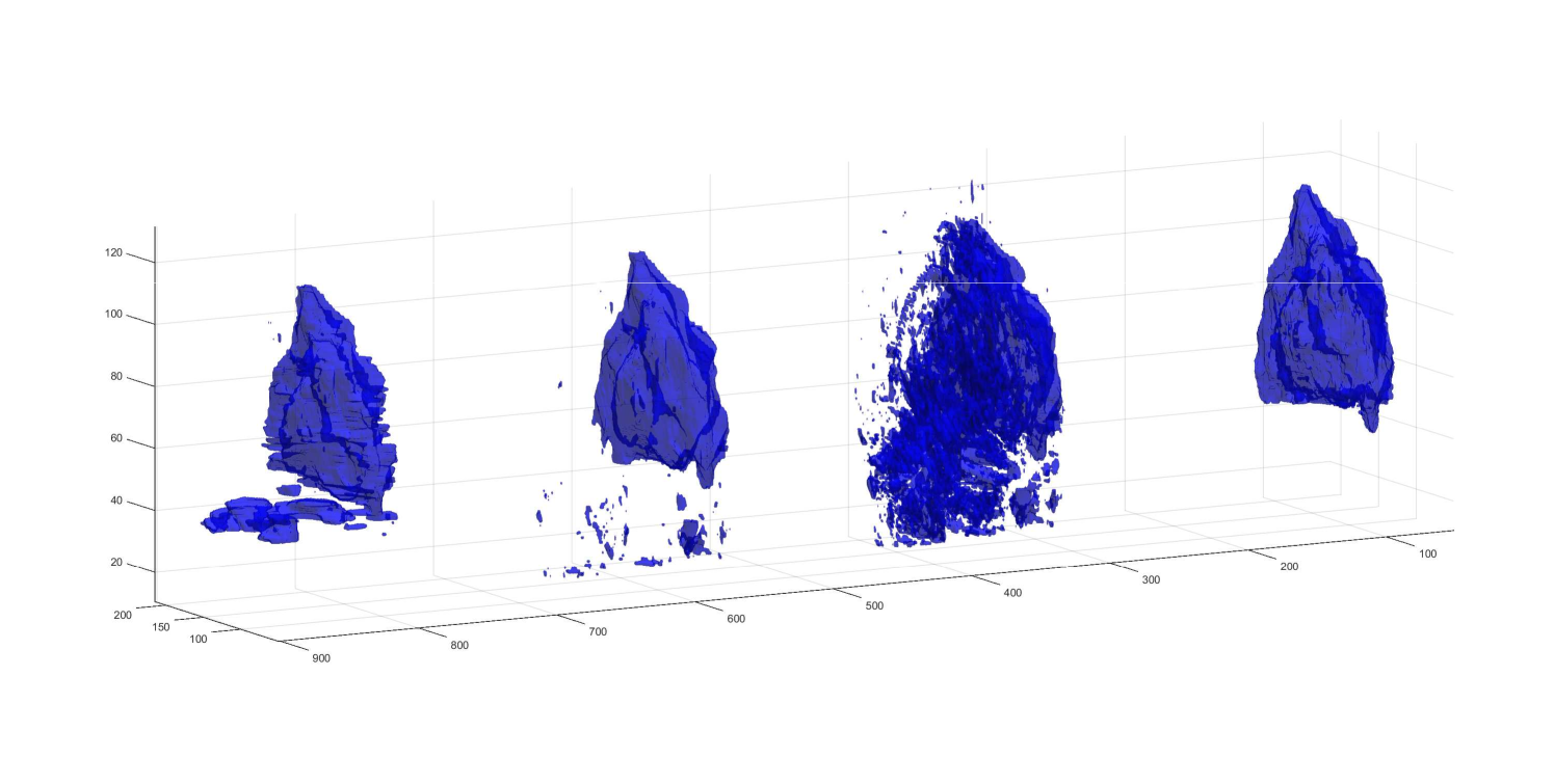
Focusing in the particular application of brain tumor segmentation, it is reasonable to think that processing each image (slice) independently will result in a sub-optimal output since no axial information is taken into account. Our model can be easily extended to process 3D brains volumes and not only 2D images (gray-scale images). In such a way, the non-local regularization will prevent from errors using 3D spatial information. The results are greatly improved as it is reported in table 2 and shown in figure 5. It is easy to see that some artifacts arise when processing the volume per slice (2D , first image), which disappear if a 3D processing is considered (second image). False positives can also be avoided in this 3D approach obtaining a cleaner image that results in a very high accuracy in common metrics (Precision, Recall and DICE, see table 2).
However, even thought the results show promising performance using this 3D scheme in comparison to a 2D processing so improving the final segmentation, the real challenge consists of choosing a correct and robust -parameter feasible for the whole volume. This is due to the non-homogeneous contrast and illumination in different regions of the MRI image which depends on the acquisition step. In future work, we will introduce some recent advances in Deep-Learning parameter estimation to obtain the optimal model parametrization which can enhance further the performance of our model (see [20]).
| Precision | Recall | DICE | |
|---|---|---|---|
| Naive Threshold | 0.5321 | 0.8008 | 0.6393 |
| 2D | 0.8658 | 0.7986 | 0.8308 |
| 3D | 0.9649 | 0.8656 | 0.9125 |
7 Conclusions
Dealing with recent challenging problems such as automatic saliency detection of videos or fixed 2D images we propose a new approach based on reactive flows which facilitates the saliency detection task promoting binary solutions which encapsulate the underlying classification problem. This is performed in a non-local framework where a bilateral filter is designed using the NLTV operator. The resulting model is numerically compared with a family of non-smooth non-local non-convex hyper-Laplacian operators. The computational cost of the model problem solving algorithm is greatly alleviated by using recent ideas on quantized convolutional operators filters making the approach practical and efficient. Numerical computations on real data sets in the modality of MRI-Flair glioblastoma automatic detection show the performance of the method.
In this work we have presented a new non-local non-convex diffusion model for saliency detection and classification which has shown to be able to perform a fast foreground detection when it is applied to a FLAIR given image. The results reveal that this method can achieve very high accurate statistics metrics over the ground-truth BRATS2015 data-set [16]. Also, as a by-product of the reactive model, the solution has, after few iterations, a reduced number of quantized values making simpler the final thresholding step. Such a technique could be improved computationally by observing that the diffusion process combined with the saliency term evolves producing more cartoon like piece-wise constant solutions which can be coded with less number of quantization values while converging to a binary mask. This is related to the absorption-reaction balance in the PDE where absorption is active where the solution is small, and the reaction is active where . The non-local diffusion properties of the model also allow to detect salient objects which are not spatially close as well as connected regions (disjoint areas). This can be useful in many other medical images modalities, specially in functional MRI (fMRI). Non-convex properties, meanwhile, promote sparse non-local gradient, pushing the solution to a cartoon piece-wise constant image. Both characteristics combined with our proposed concave energy term results in a promising accurate and fast technique suitable to be applied to FLAIR images and others MRI modalities.
ACKNOWLEDGMENTS
The first and the last authors’ research has been partially supported by the Spanish Government research funding ref. MINECO/FEDER TIN2015-69542-C2-1 and the Banco de Santander and Universidad Rey Juan Carlos Funding Program for Excellence Research Groups ref. “Computer Vision and Image Processing (CVIP)”. The second author has been supported by the Spanish MCI Project MTM2017-87162-P.
References
- [1] Ambrosio, L., Fusco, N., Pallara, D.: Functions of bounded variation and free discontinuity problems, vol. 254. Clarendon Press Oxford (2000)
- [2] Andreu-Vaillo, F.: Nonlocal diffusion problems. 165. American Mathematical Soc. (2010)
- [3] Bell, J.B.: Solutions of ill-posed problems. (1978)
- [4] Bylinskii, Z., Judd, T., Borji, A., Itti, L., Durand, F., Oliva, A., Torralba, A.: Mit saliency benchmark
- [5] Chambolle, A., Lions, P.L.: Image recovery via total variation minimization and related problems. Numerische Mathematik 76(2), 167–188 (1997)
- [6] Galiano, G., Schiavi, E., Velasco, J.: Well-posedness of a nonlinear integro-differential problem and its rearranged formulation. Nonlinear Analysis: Real World Applications 32, 74–90 (2016)
- [7] Galiano, G., Velasco, J.: On a fast bilateral filtering formulation using functional rearrangements. Journal of Mathematical Imaging and Vision 53(3), 346–363 (2015)
- [8] Ginzburg, V.L.: On the theory of superconductivity. Il Nuovo Cimento (1955-1965) 2(6), 1234–1250 (1955)
- [9] Harel, J., Koch, C., Perona, P.: Graph-based visual saliency. In: Advances in neural information processing systems, pp. 545–552 (2007)
- [10] Hintermüller, M., Wu, T.: A smoothing descent method for nonconvex tv ˆ q -models. In: Efficient Algorithms for Global Optimization Methods in Computer Vision, pp. 119–133. Springer (2014)
- [11] Krishnan, D., Fergus, R.: Fast image deconvolution using hyper-laplacian priors. In: Advances in Neural Information Processing Systems, pp. 1033–1041 (2009)
- [12] Li, M., Zhan, Y., Zhang, L.: Nonlocal variational model for saliency detection. Mathematical Problems in Engineering 2013 (2013)
- [13] Liu, R., Cao, J., Lin, Z., Shan, S.: Adaptive partial differential equation learning for visual saliency detection. In: Proceedings of the IEEE conference on computer vision and pattern recognition, pp. 3866–3873 (2014)
- [14] Liu, Z., Meur, L., Luo, S.: Superpixel-based saliency detection. In: Image Analysis for Multimedia Interactive Services (WIAMIS), 2013 14th International Workshop on, pp. 1–4. IEEE (2013)
- [15] Martín, A., Schiavi, E., de León, S.S.: On 1-laplacian elliptic equations modeling magnetic resonance image rician denoising. Journal of Mathematical Imaging and Vision 57(2), 202–224 (2017)
- [16] Menze, B.H., Jakab, A., Bauer, S., Kalpathy-Cramer, J., Farahani, K., Kirby, J., Burren, Y., Porz, N., Slotboom, J., Wiest, R., et al.: The multimodal brain tumor image segmentation benchmark (brats). IEEE transactions on medical imaging 34(10), 1993–2024 (2015)
- [17] Murea, C.M., Tiba, D.: A penalization method for the elliptic bilateral obstacle problem. In: IFIP Conference on System Modeling and Optimization, pp. 189–198. Springer (2013)
- [18] Pérez-LLanos, M., Rossi, J.D.: Numerical approximations for a nonlocal evolution equation. SIAM Journal on Numerical Analysis 49(5), 2103–2123 (2011)
- [19] Powers, D.M.: Evaluation: from precision, recall and f-measure to roc, informedness, markedness and correlation (2011)
- [20] Ramírez, I., Martín, A., Schiavi, E.: Optimization of a variational model using deep learning: an application to brain tumor segmentation. In: Biomedical Imaging (ISBI 2018), 2018 IEEE 15th International Symposium on, pp. –. IEEE (2018)
- [21] Rudin, L.I., Osher, S., Fatemi, E.: Nonlinear total variation based noise removal algorithms. Physica D: nonlinear phenomena 60(1-4), 259–268 (1992)
- [22] Rueda, A., González, F., Romero, E.: Saliency-based characterization of group differences for magnetic resonance disease classification. Dyna 80(178), 21–28 (2013)
- [23] Thota, R., Vaswani, S., Kale, A., Vydyanathan, N.: Fast 3d salient region detection in medical images using gpus. In: Machine Intelligence and Signal Processing, pp. 11–26. Springer (2016)
- [24] Tomasi, C., Manduchi, R.: Bilateral filtering for gray and color images. In: Computer Vision, 1998. Sixth International Conference on, pp. 839–846. IEEE (1998)
- [25] Wang, Y., Liu, R., Song, X., Su, Z.: Saliency detection via nonlocal l_ 0 minimization. In: Asian Conference on Computer Vision, pp. 521–535. Springer (2014)
- [26] Yang, Q., Tan, K.H., Ahuja, N.: Real-time o (1) bilateral filtering. In: Computer Vision and Pattern Recognition, 2009. CVPR 2009. IEEE Conference on, pp. 557–564. IEEE (2009)
- [27] Zhan, Y.: The nonlocal-laplacian evolution for image interpolation. Mathematical Problems in Engineering 2011 (2011)