Non-equilibrium cumulants within model A from crossover to first-order phase transition side
Abstract
We study the non-equilibrium cumulants of the chiral order parameter field ( field) in different phase transition scenarios via Langevin dynamics. Cumulants up to fourth-order have been calculated based on the spacetime-dependent configurations from the event-by-event numerical simulations. By limiting the cooling of the system in a Hubble-like way, the out-of-equilibrium cumulants illustrate clear memory effects during the evolution. Both the signs and the magnitudes of the high-order cumulants differ from the equilibrium ones below the phase transition temperature. Especially, the dynamical cumulants grow more intensively from the first-order phase transition side than they do from the crossover side. In addition, analysis of the high-order off-equilibrium cumulants on the hypothetical freeze-out lines present non-monotonic curves in the large chemical potential region.
1 Introduction
Searching for the location of the critical point and depicting the QCD phase diagram is one of the fundamental topics in heavy-ion physics, which has been extensively studied for decades Klevansky:1992qe ; Roberts:1994dr ; Berges:2000ew ; Karsch:2003jg ; Fukushima:2003fw ; Aoki:2006we ; Fu:2007xc ; Aoki:2009sc ; STAR:2010vob ; Qin:2010nq ; Jiang:2013yoa ; Luo:2017faz . Induced by the divergent fluctuations at the critical point, dramatic increases of the cumulants of the final state proton multiplicities in the critical region are predicted as a consequence of strong coupling between the quark matter and the chiral order parameter field (the field) Stephanov:1998dy ; Hatta:2003wn ; Stephanov:2008qz ; Athanasiou:2010kw ; Kitazawa:2012at . Even though the correlation length of the chiral order parameter will be suppressed by the finite size of the QCD fireball in heavy-ion collisions, the high-order correlators remain quite sensitive to the increase of the correlation length near the critical point since they are proportional to the high power of the correlation length Stephanov:2008qz . Especially, the quartic critical cumulant is predicted to be negative as approaching the critical point from the crossover side, but positive from the first-order phase transition side, thus the non-monotonic kurtosis along the chemical freeze-out line is expected to carry the signals of the QCD critical point in laboratory observations Stephanov:2008qz ; Asakawa:2009aj ; Friman:2011pf ; Stephanov:2011pb .
The experimental exploration of the QCD phase diagram is performed at the BNL Relativistic Heavy Ion Collider (RHIC). The STAR collaboration has measured the high-order cumulants of net proton production in Au+Au collisions for the collision energy ranging from GeV to GeV STAR:2010vob ; STAR:2013gus ; Luo:2015ewa . The experimental data of () shows a large deviation from the baselines determined by Poisson statistics and presents complex non-monotonic structure in the collision energy region below GeV Luo:2015ewa ; STAR:2020tga , which has not been fully explained in theoretical calculations until now. Meanwhile, more experimental measurements are being executed by the HADES collaboration at GSI HADES:2020wpc and by the ALICE Collaboration at the LHC ALICE:2019nbs . Future experimental facilities such as FAIR in Darmstadt, NICA in Dubna, HIAF in Huizhou and J-PARC in Tokai will further explore the details of the QCD phase transition at the (relative) low collision energy region.
Since the high-order cumulants of the protons are measured after hadrons chemically freeze-out, to identify the signals of the critical point from the experimental data, a proper freeze-out scheme near the critical point is introduced to the hydrodynamic model and the equilibrium cumulants of protons on the freeze-out surface are investigated Jiang:2015hri ; Jiang:2015cnt ; Jiang:2016duk . The resulted cumulants qualitatively describe the acceptance dependence of the experimental data and roughly fits the and data, but and are overestimated in this framework. Incontrovertibly, the off-equilibrium dynamics play an essential role in the dynamical evolution with phase transition to address the critical slowing down near a critical point Wu:2021xgu ; Berdnikov:1999ph and to reveal the domain formation at the first-order phase transition Randrup:2010ax . Indeed, the high-order cumulants vary significantly, not only in the magnitudes but also the signs, in the real-time evolution compared with the equilibrium hypothesis Mukherjee:2015swa ; Jiang:2017sni ; Jiang:2017fas ; Jiang:2017mji . Furthermore, the early time fluctuations and the critical enhancements around the critical point can be probed by the rapidity-window-dependent Gaussian cumulant Sakaida:2017rtj . In Ref. Nahrgang:2018afz , it shows that the effects of the nonlinear coupling and finite size are manifested through the reduction of the correlation length near the pseudo-critical temperature. In Ref. Rougemont:2018ivt , the well separated equilibrating time of non-hydrodynamic quasi-normal modes in different channels is investigated at the critical point by a phenomenological realistic holographic model, likely to be model B.
According to the classification of dynamic universality, the QCD chiral phase transition in heavy-ion collisions belongs to Model H, since it is governed by five conserved hydrodynamic modes Rev1977 ; Ma1976 ; Son:2004iv ; Chao:2020kcf ; Nahrgang:2020yxm ; De:2020yyx ; Schweitzer:2021iqk . Dynamical models with hydrodynamic background, such as chiral hydrodynamics Paech:2003fe ; Nahrgang:2011mg ; Nahrgang:2011vn ; Herold:2013bi ; Herold:2014zoa and Hydro+ Stephanov:2017ghc ; Rajagopal:2019xwg ; Du:2020bxp have been developed to describe the medium expansion and the critical mode evolution of QCD phase transition in heavy-ion collisions. However, besides the numerical complexities of these models, the equation of state, the transport coefficients, and the freeze-out scheme in the vicinity of the critical point still needs careful discussions. The numerical calculations of cumulants are even more challenging when the long range correlation of high-order fluctuations An:2020vri and the nonzero-momentum critical modes are considered for different phase transition scenarios, thus it is worth employing the simplified relaxational model A and/or diffusive model B Mukherjee:2015swa ; Jiang:2017sni ; Jiang:2017fas ; Jiang:2017mji ; Sakaida:2017rtj ; Nahrgang:2018afz ; Rougemont:2018ivt ; Nahrgang:2020yxm to study the dynamical phase transition at a broader chemical potential regions.
Based on the event-by-event Langevin equation, we detailed study the dynamical evolution of the field’s cumulants in different phase transition scenarios and on the hypothetical freeze-out line. Some preliminary results of the dynamical cumulants in various phase transition scenarios are provided in the proceedings Jiang:2017fas ; Jiang:2017mji . Here, more calculations and discussions are presented, including those involving the impact of the initial temperature on evolution and the dynamical cumulants on the hypothetical freeze-out lines. The paper is organized as follows: In Sec. 2, we introduce the dynamical model in detail where the necessary input parameters are exhibited to solve the stochastic equation, including the initial profile, expansion routine of temperature, damping coefficient, and the magnitude of noise. In Sec. 3, we present the numerical results of field’s cumulants along the given evolution trajectories in both the crossover and the first-order phase transition scenario. Afterward, we illuminate the results of non-equilibrium cumulants on the hypothetical freeze-out lines. In Sec. 4, we close the article by summarizing our main results and discussing future developments.
2 Model and set-ups
Linear sigma model is a QCD-inspired low energy effective theory, depicting the phase structure of strongly interacting matter in the - plane via the order parameter Jungnickel:1995fp ; Skokov:2010sf . As the mass of the field approaches to zero near the critical point, its correlation length grows to infinity. The corresponding equation of motion of the long wavelength mode is well described by the Langevin equation Nahrgang:2011mg ; Xu:1999aq ; Meistrenko:2020nwx :
| (1) |
where the effective potential of the field is explicitly written as
| (2) |
denotes the vacuum contribution and takes the form of
| (3) |
The parameters , , , and are set by the hadrons properties at zero temperature. As the chiral symmetry is spontaneously broken in the vacuum, the nonzero expectation of the field is MeV with . In reality, the chiral symmetry is explicitly broken by the light quark mass, then the linear term is included with and MeV. and the mass of is MeV by setting . The zero-point energy . Note that we have neglected the meson fluctuations of , since the mass of the triplet is finite in the critical regime. represents the contributions from the thermal quarks, which is
| (4) |
is the degeneracy factor of the quarks. The energy dispersion of the valence quark is with the dynamical quark mass Stephanov:2011pb ; Jiang:2015hri . For , the mass of the constituent quark is approximately MeV, and the corresponding proton mass MeV.
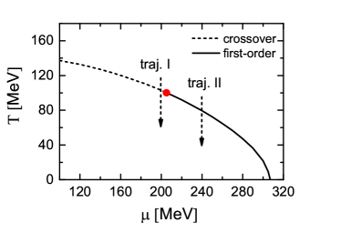
According to the effective potential of Eq. (2), the phase diagram is plotted in Fig. 1 as the function of (). The dot line denotes crossover at small , and the solid line represents the first-order phase transition at large . The critical point locates at MeV.
In Eq. (1), the damping coefficient and the white noise originate from the interaction between the field and the heat bath, which is consisted of the thermal quarks Biro:1997va . In this work, is treated as a free parameter, within the range of models allowing, whose values fm-1 are taken in the following calculations. In the zero-momentum mode limit, the correlation of the noise has the form Nahrgang:2011mg
| (5) |
We remark that the zero-momentum approximation only suits the critical point scenario at the thermodynamic limit. In the realistic case with finite correlation length, we set the spatial noise at different time steps as,
| (6) |
where is a random number generator of the standard normal distribution.
For our numerical implementation, we first construct the initial profiles of the field using the probability function: , with . In order to solve Eq. (1), the space-time information of the local temperature, , and baryon chemical potential, , have to be known which in principle shall be extracted from the heat bath. For simplicity, we assume the system evolves along the constant baryon density trajectories (seen traj. I and traj. II in Fig. 1), while the spatial-uniform temperature decreases in a Hubble-like way Mukherjee:2015swa :
| (7) |
where is the initial temperature, and fm is the initial time. The whole simulation is run in a fm3 box. The space step size fm and the time step size is fm/c. Note that the system volume will affect the configurations of field in each event, due to the change in the magnitude of the noise term, but has no influence on the results of the event-averaged .
With all the ingredients in hand, we complete the event-by-event simulations of the field from Eq. (1). In the numerical calculation process, the configurations of the field at every time step over events are recorded. The moments of the field are then calculated by:
| (8) |
where . The non-equilibrium cumulants of the field are iteratively determined by the following formula:
| (9) | |||||
| (10) | |||||
| (11) | |||||
| (12) |
3 Numerical results and discussions
3.1 dynamical evolution in the crossover scenario — critical slowing down
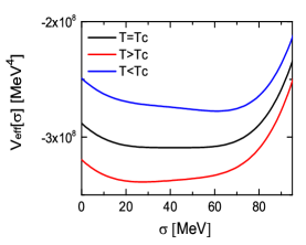
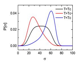
We first solve the Langevin equation in the crossover scenario for MeV. The effective potential and the probability distribution function for the phase transition region are shown in Fig. 2. Both the effective potential and the distribution function each have a dip or peak at the given temperature region. The system smoothly transits from the symmetry restored phase to the symmetry broken phase as the temperature decreases.
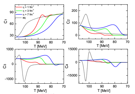
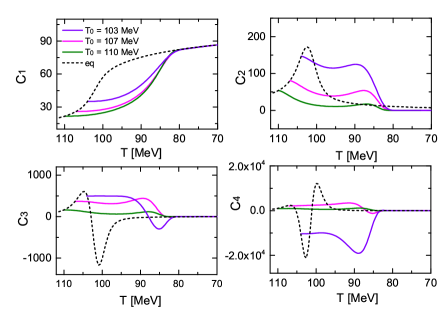
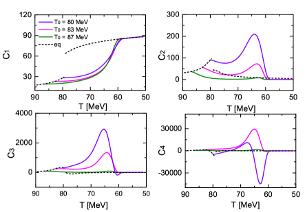
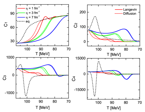
In Fig. 3, we plot the dynamical evolution of ’s cumulants along traj. I as marked on the cartoon phase diagram of Fig. 1. The corresponding horizontal axis is the inverted temperature as time increases. The dashed lines represent the equilibrium cumulants, and the colored solid lines represent the non-equilibrium ones at a given damping coefficient. In the left panel, we show the behavior of ’s cumulants at different damping coefficients. The initial configurations of fields are constructed to satisfy the equilibrium distribution at , thus both the non-equilibrium and equilibrium cumulants have the same values at the starting point. In the evolution, the non-equilibrium cumulants present clear memory effects, going after the trends of equilibrium ones as temperature decreases and reaching their maxima (or minima) at later times. Finally, after the phase transition, the effective potential changes from a non-Gaussian shape to a Gaussian shape. As expected, the non-equilibrium goes to the equilibrium value and the high-order cumulants vanish at the broken phase. During the expansion, non-equilibrium decreases slightly at the earlier stage and then grows due to the broadening of the effective potential in the critical region. We emphasize that the signs and values of the dynamical strongly differ from the equilibrium ones in a large T region below . For larger damping coefficients, the field relaxes as slowly as it should and the system takes a longer time to approach equilibrium. Prolonging the duration to its out-of-equilibrium state, the maximum (or minimum) of high-order cumulants are enhanced as increases. The effect of the damping coefficients can be estimated in the strong limit. In the critical region, the behavior of the critical mode simplifies to a diffusion-like process, as , the higher order time derivative term are ignored. Shown in Fig.7 in Appendix 1, a large results in an over-damped system, and the cumulants from the Langevin dynamics match those from the diffusion equation.
Besides the damping coefficients, the initial conditions also have a significant influence on the magnitude of the dynamical cumulants. In the right panel of Fig. 3, we exhibit the results of non-equilibrium cumulants starting from three different initial temperatures above , with the damping coefficient fixed at . The initial field configurations are again sampled according to the equilibrium distribution function and thus vary for different . Again, the initial values of the ’s cumulants are governed by the field’s distribution at starting temperature. We find that the high-order cumulants are strongly enlarged while are close to and maintain substantial values during the later non-equilibrium development until below . In addition, with the same damping coefficient, the cumulants reach their maxima (or minima) at approximately the same temperature, which is almost unrelated to their starting points.
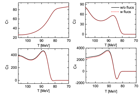
Note that we have also carried out calculations on the dynamical cumulants both with and without the spatial fluctuations of the fields, as demonstrated in Appendix 2. The influence of spatial fluctuations is diminished since we perform the statistics based on the event-averaged field. Shown in Fig. 8, for the specified values of and , we compare ’s at two cases. As evident, it is challenging to observe the impact of the spatially non-uniform field on the cumulants after event-by-event averaging.
3.2 dynamical evolution in the first-order phase transition scenario — supercooling effect
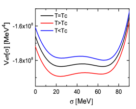
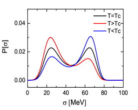
In this subsection, we discuss the dynamical evolution of ’s cumulants in the first-order phase transition scenario, with the baryon chemical potential fixed at . As shown in the left panel of Fig. 4, the thermodynamic potentials are characterized by two co-existing phases near . At the thermodynamic limit, the probability distribution function is double -like only at the phase transition point. The field stays at the global minimum of the effective potential, and there is a discontinuity at the phase transition temperature in the equilibrium cumulants. In turn, confining to a finite system volume ( fm3), the probability distribution function presents two peaks with comparable probability in the phase transition region (as shown in the right panel of Fig. 4), which leads to significantly different behaviors of the high-order cumulants.
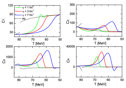
In Fig. 5, we present the numerical results of dynamical cumulants as functions of decreasing temperature, as denoted by the traj. II in Fig. 1. The left panel represents the evolution of cumulants starting from a given set of ’s configurations under different damping coefficients. For fixed , the right panel shows the cumulative behaviors starting at various initial temperatures. Similar to the case in the crossover scenario, the diffusive dynamics render the same memory effects for the non-equilibrium cumulants. In addition, the non-equilibrium cumulants are continuous and much larger than that of the equilibrium ones.
The significant enhancements of the non-equilibrium cumulants are explained in the following. In the first-order phase transition scenario, the existence of a barrier between the two minima in the thermodynamic potential prevents the ’s configurations from shrinking to the global minimum even when the temperature is lower than (known as supercooling effects in thermodynamics). Since the field is trapped in the original minima during the cooling down process, only the events with intense thermal fluctuations would overcome the potential barrier. Then as the broadening of the probability distribution function in a finite-size system, different events occupy both of the states with comparable weights, which leads to a strong departure of from the equilibrium cumulants. Such enhancements of cumulants at the boundary side of the first-order phase transition have the potential to address the large deviations of BES data from the statistical baselines at low collision energies.
3.3 cumulants on the hypothetical freeze-out lines
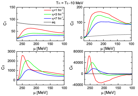
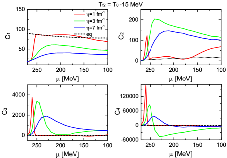
The possible signals of phase transition are measured after the particles chemically freeze out, and in this subsection, we discuss the non-equilibrium cumulants’ behaviors on the hypothetical freeze-out lines as functions of baryon chemical potential. Within the present model setting, the phase transition line described by the linear sigma model is far away from the freeze-out line determined by the statistical model via fitting experimental data Andronic:2017pug . Thus, we are not able to directly borrow the freeze-out information from the experiments. In the following, we artificially choose the freeze-out lines and assume the dynamical evolution of the field along different trajectories starting at MeV, and freezing out at either MeV or MeV. In the duration of each trajectory, the baryon chemical potential is fixed.
In Fig. 6, we draw the ’s cumulants as functions of the baryon chemical potential, adopting and as the freeze-out temperature individually. The high-order equilibrium cumulants decay to zero as the system is away from the phase transition region. Rather, the non-equilibrium cumulants exhibit large deviations from the equilibrium ones and significant non-monotonic structures on the hypothetical freeze-out line. Below , the equilibrium is negative and limited to zero as temperature decreases. However, the non-equilibrium is positive in most phase space of for both applied freeze-out lines. The flipping of signs could address the sign problem based on the prediction of equilibrium critical fluctuations Jiang:2015hri . Last but not least, the non-equilibrium is oscillating near the critical baryon chemical potential (MeV) and tends to zero around MeV.
By comparing the vanishing equilibrium cumulants of , the dynamical processes provide us with abundant nontrivial behaviors. In our model calculation, the appearance of the non-monotonic curves of originates from a combined effect of and the hypothetical freeze-out line. At the first freeze-out temperature , the evolution of at smaller (red and green lines) show the non-monotonic structure, but they oscillate under the influence of larger (green and blue lines) at freeze-out temperature . This means that evolves following its own dynamical processes and its behavior is non-universal. Furthermore, the deviation of not only comes from the development of itself but also from the non-equilibrium features of other cumulants since the higher order cumulants are coupled to the lower order ones as shown in Eq.(9-12).
The peaks of and are worth paying attention to, as well. Both of these maximums take place at a critical value around MeV. Such maximums are induced by the maximization of the supercooling effect in the current model. With slightly larger than , the barrier between the global minima and the false minima prevents a critical number of events from developing to the global minimum. The field is approximately evenly distributed in both minima for different events, and induces a dramatically large peak of the high-order cumulants. At the high baryon chemical potential, MeV, the barrier is so strong that the field is trapped in the original minima and can not escape even at a temperature much lower than . Without the fluctuations manifesting the phase transition, the high-order cumulants are suppressed, and their magnitude approaches the equilibrium limit.
In spite of the various cumulative behaviors found in the first-order phase transition scenario, we note that one should be cautious when comparing the current model simulation at a high baryon chemical potential region to the experimental data, since a mismatch between the model and the experiments at small collision energies is likely to occur. In this work, we have presumed that system evolution occurs when the chiral symmetry is restored, but quark-gluon-plasma may not be created in heavy-ion collisions at low collision energies. A sophisticated first-order phase transition with the proper degree of freedom should be further explored and studied in future work.
4 Summary and outlook
To summarize, in this work, we study the dynamical evolution of the field based on the event-by-event simulations of a single component Langevin equation. The temperature decrease for the system is set to be Hubble like and the computation is completed in a finite-size system. We statistically weight the dynamical variable over events during the real-time evolution to obtain its high-order cumulants. With the current model setting, we find that the non-equilibrium cumulants express clear memory effects, and the magnitude of slowly increases as the system approaches its critical regions. The signs of , as well as the magnitudes, can differ from the equilibrium ones below . We also find that the high-order cumulants are significantly enhanced on the boundary side of the first-order phase transition. Finally, the spread of out-of-equilibrium cumulants along the hypothetical freeze-out lines has been presented. The non-equilibrium is positive at large baryon chemical potentials, in contrast to the negative sign of the equilibrium . In the vicinity of CP, with certain parameter sets, the non-equilibrium expresses non-monotonic curves at large region. We conclude that the combination of supercooling effect and dynamical effects on the first-order phase transition side plays a dominant role in the nonmonotonicity of the high-order cumulants on the hypothetical freeze-out lines.
Note that the apparent memory effects of the cumulants up to the fourth order based on the Langevin framework are in accord with those obtained by the use of the Fokker-Plank equations Mukherjee:2015swa ; Jiang:2017sni , but currently not sufficiently discussed and presented elsewhere, which is crucial for the study of nonequilibrium signals from experiments. Of course, in order to quantitatively describe the experimentally observed cumulants of net proton multiplicities, more sophisticated and realistic dynamical modeling are required from the theoretical side Kapusta:2011gt ; Akamatsu:2017rdu . A suitable mathematical tool that can accurately describe the properties of fluids in heavy-ion collisions and better performs numerical calculations is still under exploration. It is well known that the method of Fokker-Plank equations is equivalent to the Langevin dynamics in the Markov process Mukherjee:2015swa ; Jiang:2017sni ; An:2021wof . However, taking into account the realistic fireball evolution in heavy-ion collisions, where the spatial distributions of temperature and baryon chemical potential, etc., are nonuniform, the Langevin dynamics has the advantage of easily including those effects in simulations, and further combines with the hydrodynamic equations to describe the complete dynamical process in RHIC. We note here how these non-Markov effects manifest in the Fokker-Plank equations is beyond the scope of this paper. Further investigation and analysis are under work.
In this paper, with a relatively simple setup for the modeling and the parameters, we present the dynamics of the cumulants, which serves as reference information for the analysis of the experimental measurements. For the explanation of the experimental data, a number of effects are playing their roles, including the subject of the proper equation of state Monnai:2019hkn ; Noronha-Hostler:2019ayj ; Parotto:2018pwx , of the unknown parameters of the Ising-to-QCD mapping Mroczek:2020rpm , of the critical transport coefficients Karpenko:2015xea ; Denicol:2015nhu ; Bernhard:2019bmu ; Martinez:2019bsn , of the finite size, finite size scaling and global charge conservation in the vicinity of a CP Sombun:2017bxi ; Antoniou:2017vti ; Vovchenko:2020gne ; Poberezhnyuk:2020ayn ; Tomasik:2021jfd , of the non-critical baselines for the cumulants of net-proton number fluctuations Braun-Munzinger:2020jbk , of the nonuniform temperature/chemical potential effects Zheng:2021pia , and of the proper freezeout scheme in the critical region Pradeep:2022mkf . Besides, further connections between the criticality and the other experimental observable are being established through theoretical efforts Mukherjee:2016kyu ; Sun:2017xrx ; Sun:2018jhg ; Wu:2018twy ; Brewer:2018abr ; Pratt:2019fbj and new technique such as the machine learning method Pang:2016vdc ; Huang:2018fzn ; Jiang:2021gsw is also being developed for the search of QCD phase transition signals as well.
APPENDIX
1. the comparison of dynamical results from diffusion equation and Langevin equation
In the low frequency range, the evolution of the sigma field is described by an over-damped diffusion-like equation, since . Ignoring the second order time derivative term, the diffusion equation takes the form:
| (13) |
Here we compare the numerical evolution of the sigma field using the Langevin equation as well as the over-damped diffusion equation. In Fig. 7, we plot the Langevin (solid lines) dynamics of ’s cumulants and the over-damped diffusion equation (dotted lines) with three different damping coefficients at MeV. In the figure, it is shown that the differences of ’s cumulants decrease with an increase in the damping coefficient. At , the evolution differences between the two kinds of equations can be safely ignored.
2. the comparison of dynamical cumulants with and without spatial fluctuations
Here, we numerically simulate the dynamical cumulants under the assumption that the sigma field is spatially homogeneous (the black lines in Fig. 8) and compare the results to the cases with spatial fluctuations (red dashed lines in Fig. 8). It has been discovered that there are no apparent differences between the first and second-order cumulants. The third and fourth-order cumulants have larger magnitudes in the early stages for the spatially uniform events, but the differences reduce in later stages due to the damping of the field. Thus based on the above calculations, we find that it is difficult to detect the impact of ’s spatial fluctuations on the event-averaged quantities.
Acknowledgements
We thank Ulrich. Heinz, Yu-Xin Liu, Swagato Mukherjee, Misha Stephanov, Derek Teaney, Yi Yin, Shanjin Wu and Huichao Song for useful discussion and comments. We thank the anonymous reviewer for his/her valuable suggestions in the impact of spatial non-uniformity of the sigma field. The work of LJ has been supported by the NSFC under grant no. 12105223, and the work of JC has been supported by the start-up funding from Jiangxi Normal University under grant No. 12021211.
References
- (1) S. P. Klevansky, The Nambu-Jona-Lasinio model of quantum chromodynamics, Rev. Mod. Phys. 64, 649 (1992).
- (2) C. D. Roberts and A. G. Williams, Dyson-Schwinger equations and their application to hadronic physics, Prog. Part. Nucl. Phys. 33, 477 (1994).
- (3) J. Berges, N. Tetradis, and C. Wetterich, Non-perturbative renormalization flow in quantum field theory and statistical physics, Phys. Rept. 363, 223 (2002).
- (4) F. Karsch and E. Laermann, Thermodynamics and in-medium hadron properties from lattice QCD, Quark gluon plasma 3, 1 (2004) (Edited by R.C. Hwa, and X.-N. Wang); hep-lat/0305025 (2003).
- (5) K. Fukushima, Chiral effective model with the Polyakov loop, Phys. Lett. B 591, 277 (2004).
- (6) Y. Aoki, G. Endrodi, Z. Fodor, S. D. Katz, and K. K. Szabó, The order of the quantum chromodynamics transition predicted by the standard model of particle physics, Nature 443, 675 (2006).
- (7) Y. Aoki, S. Borsányi, S. Dürr, Z. Fodor, S. D. Katz, S. Krieg, and K. K. Szabo, The QCD transition temperature: results with physical masses in the continuum limit II, JHEP 0906, 088 (2009).
- (8) W.-j. Fu, Z. Zhang, and Y.-x. Liu, 2+1 flavor Polyakov-Nambu-Jona-Lasinio model at finite temperature and nonzero chemical potential, Phys. Rev. D 77, 014006 (2008).
- (9) M. M. Aggarwal et al. [STAR Collaboration], An experimental exploration of the QCD phase diagram: the search for the critical point and the onset of de-confinement, arXiv:1007.2613 (2010).
- (10) S.-x. Qin, L. Chang, H. Chen, Y.-x. Liu, and C. D. Roberts, Phase diagram and critical end point for strongly interacting quarks, Phys. Rev. Lett. 106, 172301 (2011).
- (11) L.-j. Jiang, X.-y. Xin, K.-l. Wang, S.-x. Qin, and Y.-x. Liu, Revisiting the phase diagram of the three-flavor quark system in the Nambu-Jona-Lasinio model, Phys. Rev. D 88, 016008 (2013).
- (12) X. Luo and N. Xu, Search for the QCD critical point with fluctuations of conserved quantities in relativistic heavy-ion collisions at RHIC : an overview, Nucl. Sci. Tech. 28, 112 (2017).
- (13) M. A. Stephanov, K. Rajagopal and E. V. Shuryak, Signatures of the tricritical point in QCD, Phys. Rev. Lett. 81, 4816 (1998).
- (14) Y. Hatta and M. A. Stephanov, Proton number fluctuation as a signal of the QCD critical endpoint, Phys. Rev. Lett. 91, 102003 (2003); Erratum: Phys. Rev. Lett. 91, 129901 (2003)].
- (15) M. A. Stephanov, Non-Gaussian fluctuations near the QCD critical point, Phys. Rev. Lett. 102, 032301 (2009).
- (16) C. Athanasiou, K. Rajagopal, and M. Stephanov, Using higher moments of fluctuations and their ratios in the search for the QCD critical point, Phys. Rev. D 82, 074008 (2010).
- (17) M. Kitazawa and M. Asakawa, Relation between baryon number fluctuations and experimentally observed proton number fluctuations in relativistic heavy ion collisions, Phys. Rev. C 86, 024904 (2012); Erratum: Phys. Rev. C 86, 069902 (2012).
- (18) M. Asakawa, S. Ejiri and M. Kitazawa, Third moments of conserved charges as probes of QCD phase structure, Phys. Rev. Lett. 103 (2009), 262301
- (19) B. Friman, F. Karsch, K. Redlich and V. Skokov, Fluctuations as probe of the QCD phase transition and freeze-out in heavy ion collisions at LHC and RHIC, Eur. Phys. J. C 71,1694 (2011).
- (20) M. A. Stephanov, Sign of kurtosis near the QCD critical point, Phys. Rev. Lett. 107, 052301 (2011).
- (21) L. Adamczyk et al. [STAR Collaboration], Energy dependence of moments of net-proton multiplicity distributions at RHIC, Phys. Rev. Lett. 112, 032302 (2014).
- (22) X. Luo [STAR Collaboration], Energy dependence of moments of net-proton and net-charge multiplicity distributions at STAR, PoS CPOD 2014, 019 (2014).
- (23) J. Adam et al. [STAR Collaboration], Nonmonotonic energy dependence of net-proton number fluctuations, Phys. Rev. Lett. 126, 092301 (2021).
- (24) J. Adamczewski-Musch et al. [HADES], Proton-number fluctuations in =2.4 GeV Au + Au collisions studied with the High-Acceptance DiElectron Spectrometer (HADES), Phys. Rev. C 102, 024914 (2020).
- (25) S. Acharya et al. [ALICE], Global baryon number conservation encoded in net-proton fluctuations measured in Pb-Pb collisions at = 2.76 TeV, Phys. Lett. B 807, 135564 (2020).
- (26) L. Jiang, P. Li, and H. Song, Correlated fluctuations near the QCD critical point, Phys. Rev. C 94, 024918 (2016).
- (27) L. Jiang, P. Li and H. Song, Multiplicity fluctuations of net protons on the hydrodynamic freeze-out surface, Nucl. Phys. A 956, 360 (2016).
- (28) L. Jiang, P. Li and H. Song, Static critical fluctuations on the freeze-out surface, Acta Phys. Polon. Supp. 10, 603 (2017).
- (29) S. Wu, C. Shen and H. Song, Dynamically Exploring the QCD Matter at Finite Temperatures and Densities: A Short Review, Chin. Phys. Lett. 38, 081201 (2021).
- (30) B. Berdnikov and K. Rajagopal, Slowing out of equilibrium near the QCD critical point, Phys. Rev. D 61, 105017 (2000).
- (31) J. Randrup, Spinodal phase separation in relativistic nuclear collisions, Phys. Rev. C 82, 034902 (2010).
- (32) S. Mukherjee, R. Venugopalan, and Y. Yin, Real-time evolution of non-Gaussian cumulants in the QCD critical regime, Phys. Rev. C 92, 034912 (2015).
- (33) L. Jiang, H. Stoecker and J. H. Zheng, Eur. Phys. J. C 83 (2023) no.2, 117 doi:10.1140/epjc/s10052-023-11261-z
- (34) L. Jiang, S. Wu, and H. Song, Enhancements of high order cumulants across the 1st order phase transition boundary, EPJ Web Conf. 171, 16003 (2018).
- (35) L. Jiang, S. Wu, and H. Song, Dynamical fluctuations in critical regime and across the 1st order phase transition, Nucl. Phys. A 967, 441 (2017).
- (36) M. Sakaida, M. Asakawa, H. Fujii, and M. Kitazawa, Dynamical evolution of critical fluctuations and its observation in heavy ion collisions, Phys. Rev. C 95, 064905 (2017).
- (37) M. Nahrgang, M. Bluhm, T. Schaefer, and S. A. Bass, Diffusive dynamics of critical fluctuations near the QCD critical point, Phys. Rev. D 99, 116015 (2019).
- (38) R. Rougemont, R. Critelli and J. Noronha, Nonhydrodynamic quasinormal modes and equilibration of a baryon dense holographic QGP with a critical point, Phys. Rev. D 98, 034028 (2018).
- (39) P. C. Hohenberg, and B. I. Halperin, Theory of dynamic critical phenomena, Rev. Mod. Phys. 49, 435 (1977).
- (40) S. K. Ma, Modern theory of critical phenomena, Westview Press (1976).
- (41) D. T. Son and M. A. Stephanov, Dynamic universality class of the QCD critical point, Phys. Rev. D 70, 056001 (2004).
- (42) J. Chao and T. Schaefer, Multiplicative noise and the diffusion of conserved densities, JHEP 01, 071 (2021).
- (43) M. Nahrgang and M. Bluhm, Modeling the diffusive dynamics of critical fluctuations near the QCD critical point, Phys. Rev. D 102, 094017 (2020).
- (44) A. De, C. Plumberg and J. I. Kapusta, Calculating fluctuations and self-correlations numerically for causal charge diffusion in relativistic heavy-ion collisions, Phys. Rev. C 102, 024905 (2020).
- (45) D. Schweitzer, S. Schlichting and L. von Smekal, Critical dynamics of relativistic diffusion, arXiv:2110.01696.
- (46) K. Paech, H. Stöcker, and A. Dumitru, Hydrodynamics near a chiral critical point, Phys. Rev. C 68, 044907 (2003).
- (47) M. Nahrgang, S. Leupold, C. Herold, and M. Bleicher, Nonequilibrium chiral fluid dynamics including dissipation and noise, Phys. Rev. C 84, 024912 (2011).
- (48) M. Nahrgang, C. Herold, S. Leupold, I. Mishustin, and M. Bleicher, The impact of dissipation and noise on fluctuations in chiral fluid dynamics, J. Phys. G 40, 055108 (2013).
- (49) C. Herold, M. Nahrgang, I. Mishustin, and M. Bleicher, Chiral fluid dynamics with explicit propagation of the Polyakov loop, Phys. Rev. C 87, 014907 (2013).
- (50) C. Herold, M. Nahrgang, Y. Yan and C. Kobdaj, Net-baryon number variance and kurtosis within nonequilibrium chiral fluid dynamics, J. Phys. G 41, no.11, 115106 (2014).
- (51) M. Stephanov and Y. Yin, Hydrodynamics with parametric slowing down and fluctuations near the critical point, Phys. Rev. D 98, 036006 (2018).
- (52) K. Rajagopal, G. Ridgway, R. Weller and Y. Yin, Understanding the out-of-equilibrium dynamics near a critical point in the QCD phase diagram, Phys. Rev. D 102, 094025 (2020).
- (53) L. Du, U. Heinz, K. Rajagopal, and Y. Yin, Fluctuation dynamics near the QCD critical point, Phys. Rev. C 102, 054911 (2020).
- (54) X. An, G. Başar, M. Stephanov, and H. U. Yee, Evolution of Non-Gaussian Hydrodynamic Fluctuations, Phys. Rev. Lett. 127, 072301 (2021).
- (55) D. U. Jungnickel and C. Wetterich, Effective action for the chiral quark-meson model, Phys. Rev. D 53, 5142 (1996).
- (56) V. Skokov, B. Friman, E. Nakano, K. Redlich and B. J. Schaefer, Vacuum fluctuations and the thermodynamics of chiral models, Phys. Rev. D 82, 034029 (2010).
- (57) Z. Xu and C. Greiner, Stochastic treatment of disoriented chiral condensates within a Langevin description, Phys. Rev. D 62, 036012 (2000).
- (58) A. Meistrenko, H. van Hees and C. Greiner, Kinetics of the chiral phase transition in a quark–meson -model, Annals Phys. 431, 168555 (2021).
- (59) T. S. Biro and C. Greiner, Dissipation and fluctuation at the chiral phase transition, Phys. Rev. Lett. 79, 3138 (1997)
- (60) A. Andronic, P. Braun-Munzinger, K. Redlich and J. Stachel, Decoding the phase structure of QCD via particle production at high energy, Nature 561, 321 (2018).
- (61) X. An, M. Bluhm, L. Du, G. V. Dunne, H. Elfner, C. Gale, J. Grefa, U. Heinz, A. Huang and J. M. Karthein, et al. The BEST framework for the search for the QCD critical point and the chiral magnetic effect, Nucl. Phys. A 1017, 122343 (2022).
- (62) J. I. Kapusta, B. Muller and M. Stephanov, Relativistic Theory of Hydrodynamic Fluctuations with Applications to Heavy Ion Collisions,Phys. Rev. C 85, 054906 (2012).
- (63) Y. Akamatsu, A. Mazeliauskas and D. Teaney, Bulk viscosity from hydrodynamic fluctuations with relativistic hydrokinetic theory, Phys. Rev. C 97, 024902 (2018).
- (64) A. Monnai, B. Schenke, and C. Shen, Equation of state at finite densities for QCD matter in nuclear collisions, Phys. Rev. C 100, 024907 (2019).
- (65) J. Noronha-Hostler, P. Parotto, C. Ratti, and J. M. Stafford, Lattice-based equation of state at finite baryon number, electric charge and strangeness chemical potentials, Phys. Rev. C 100, 064910 (2019).
- (66) P. Parotto, M. Bluhm, D. Mroczek, M. Nahrgang, J. Noronha-Hostler, K. Rajagopal, C. Ratti, T. Schäfer, and M. Stephanov, QCD equation of state matched to lattice data and exhibiting a critical point singularity, Phys. Rev. C 101, 034901 (2020).
- (67) D. Mroczek, A. R. Nava Acuna, J. Noronha-Hostler, P. Parotto, C. Ratti, and M. A. Stephanov, Quartic cumulant of baryon number in the presence of a QCD critical point, Phys. Rev. C 103, 034901 (2021).
- (68) I. A. Karpenko, P. Huovinen, H. Petersen and M. Bleicher, Estimation of the shear viscosity at finite net-baryon density from collision data at GeV, Phys. Rev. C 91, 064901 (2015).
- (69) G. Denicol, A. Monnai and B. Schenke, Moving forward to constrain the shear viscosity of QCD matter, Phys. Rev. Lett. 116, 212301 (2016).
- (70) J. Bernhard, J. S. Moreland and S. A. Bass, Bayesian estimation of the specific shear and bulk viscosity of quark–gluon plasma, Nature Phys.15, 1113. (2019).
- (71) M. Martinez, T. Schäfer and V. Skokov, Critical behavior of the bulk viscosity in QCD, Phys. Rev. D 100, 074017 (2019).
- (72) S. Sombun, J. Steinheimer, C. Herold, A. Limphirat, Y. Yan and M. Bleicher, Higher order net-proton number cumulants dependence on the centrality definition and other spurious effects, J. Phys. G 45, 025101 (2018).
- (73) N. G. Antoniou, F. K. Diakonos, X. N. Maintas and C. E. Tsagkarakis, Locating the QCD critical endpoint through finite-size scaling, Phys. Rev. D 97, 034015 (2018).
- (74) V. Vovchenko, R. V. Poberezhnyuk and V. Koch, Cumulants of multiple conserved charges and global conservation laws, JHEP 10, 089 (2020).
- (75) R. V. Poberezhnyuk, O. Savchuk, M. I. Gorenstein, V. Vovchenko, K. Taradiy, V. V. Begun, L. Satarov, J. Steinheimer and H. Stoecker, Critical point fluctuations: Finite size and global charge conservation effects, Phys. Rev. C 102, 024908 (2020).
- (76) B. Tomasik, P. Hillmann and M. Bleicher, Proton number fluctuations in partial chemical equilibrium, Phys. Rev. C 104, 044907 (2021).
- (77) P. Braun-Munzinger, B. Friman, K. Redlich, A. Rustamov and J. Stachel, Relativistic nuclear collisions: Establishing a non-critical baseline for fluctuation measurements, Nucl. Phys. A 1008, 122141 (2021).
- (78) J.-H. Zheng and L. Jiang, Nonuniform-temperature effects on the phase transition in an Ising-like model, Phys. Rev. D 104, 016031 (2021).
- (79) M. Pradeep, K. Rajagopal, M. Stephanov, and Y. Yin, Freezing out gluctuations in Hydro+ near the QCD critical point, Phys. Rev. D 106, 036017 (2022).
- (80) S. Mukherjee, R. Venugopalan and Y. Yin, Universal off-equilibrium scaling of critical cumulants in the QCD phase diagram, Phys. Rev. Lett. 117, 222301 (2016).
- (81) K.-J. Sun, L.-W. Chen, C. M. Ko and Z. Xu, Probing QCD critical fluctuations from light nuclei production in relativistic heavy-ion collisions, Phys. Lett. B 774, 103 (2017).
- (82) K.-J. Sun, L.-W. Chen, C. M. Ko, J. Pu and Z. Xu, Light nuclei production as a probe of the QCD phase diagram, Phys. Lett. B 781, 499 (2018).
- (83) S. Wu, Z. Wu and H. Song, Universal scaling of the field and net-protons from Langevin dynamics of model A, Phys. Rev. C 99, 064902 (2019).
- (84) J. Brewer, S. Mukherjee, K. Rajagopal and Y. Yin, Searching for the QCD critical point via the rapidity dependence of cumulants, Phys. Rev. C 98, 061901 (2018).
- (85) S. Pratt, Calculating -Point Charge Correlations in Evolving Systems, Phys. Rev. C 101, 014914 (2020).
- (86) L. G. Pang, K. Zhou, N. Su, H. Petersen, H. Stöcker and X. N. Wang, An equation-of-state-meter of quantum chromodynamics transition from deep learning, Nature Commun. 9, 210 (2018).
- (87) H. Huang, B. Xiao, Z. Liu, Z. Wu, Y. Mu and H. Song, Applications of deep learning to relativistic hydrodynamics, Phys. Rev. Res. 3, 023256 (2021).
- (88) L. Jiang, L. Wang and K. Zhou, Deep learning stochastic processes with QCD phase transition, Phys. Rev. D 103, 116023 (2021).