Non-equilibrium Ensembles for the three-dimensional Navier-Stokes equations
Abstract
At the molecular level fluid motions are, by first principles, described by time reversible laws. On the other hand, the coarse grained macroscopic evolution is suitably described by the Navier-Stokes equations, which are inherently irreversible, due to the dissipation term. Here, a reversible version of three-dimensional Navier-Stokes is studied, by introducing a fluctuating viscosity constructed in such a way that enstrophy is conserved, along the lines of the paradigm of microcanonical versus canonical treatment in equilibrium statistical mechanics. Through systematic simulations we attack two important questions: (a) What are the conditions that must be satisfied in order to have a statistical equivalence between the two non-equilibrium ensembles? (b) What is the empirical distribution of the fluctuating viscosity observed by changing the Reynolds number and the number of modes used in the discretization of the evolution equation? The latter point is important also to establish regularity conditions for the reversible equations. We find that the probability to observe negative values of the fluctuating viscosity becomes very quickly extremely small when increasing the effective Reynolds number of the flow in the fully resolved hydro dynamical regime, at difference from what was observed previously.111Post-print version of the article published in Phys. Rev. E, 105(6), 065110, (2022).
pacs:
47.10.ad Navier-Stokes equations; 47.27.E- Turbulence simulation and modeling; 05.40.-a Fluctuation phenomena, random processes, noise, and Brownian motionI Introduction
The statistical balance between energy injection and dissipation is the key ingredient for the establishment of steady state conditions in non-equilibrium statistical mechanical systems. Such systems are driven out of equilibrium by the presence of an external forcing, while dissipation acts as a thermostat that removes the excess of energy (1; 2), with entropy being produced in the process.
In the case of fluid systems, described by the Navier-Stokes equation (NSE) (3; 4), dissipation is introduced in the form of a Laplacian operator acting on the velocity field times a positive constant: the viscosity. Such an operator preferentially damps the small scales of the flow. There are other ways to introduce dissipation, and two relevant examples are given next. For instance, in two-dimensional (2D) and geophysical flows, dissipation is often introduced via the Ekman friction, which is justified, e.g., by the effects of the bottom and top surfaces of the thin fluid layer which helps avoiding accumulation of energy at large scales (5; 6). Another approach, used customarily in numerical simulations to reach high intensity turbulent states in many applications, is to introduce hyperviscosity (7), i.e., a positive power of the Laplacian, which confines dissipation to the small scales, acting, de facto, like a sharp ultraviolet filter. It is also possible to introduce dissipation by combining more than one of the above outlined approaches. The common characteristic among all the forms of dissipation described above is that they break the time reversal symmetry, which is instead preserved by the other terms of the NSE.
Reversible equations govern microscopic motion while irreversible equations describe, very often, macroscopic evolution of the same systems with equations derived via scaling of various parameters (8; 9; 10; 11). Thus, the question arises as to whether the macroscopic description of systems evolving irreversibly could also be described macroscopically by reversible equations.
The equivalence of different ensembles in equilibrium statistical mechanics (see, e.g., (12; 13)) describes, in the thermodynamic limit, the independence of macroscopic observables with respect to the chosen thermostat, which defines the underlying microscopic interactions between the system and the reservoir in contact with it. In non-equilibrium systems it is possible to appropriately modify the irreversible term(s) of the evolution equation in such a way that time reversibility is restored, while, under suitable constraints, a macroscopic quantity is kept fixed (14); an early example for NSE is in (15) where many conditions are simultaneously imposed to constrain that the energy content obeys at every scale (above the Kolmogorov’s) the law. The key question is whether, and under which conditions, the two ensembles (irreversible and reversible) are equivalent and describe the same physical problem.
In the context of fluid systems, where the viscous term is the source of irreversibility, it is possible to introduce a velocity field-dependent fluctuating viscosity, such that the viscous term becomes formally reversible, while keeping fixed a macroscopic quantity (e.g. the energy or enstrophy, etc.) as a constraint. The equivalence between the irreversible and reversible fluid ensembles was first conjectured in (16; 17) in the limit of vanishing viscosity and fixed system size. Subsequent numerical attempts addressed this conjecture in a few simple systems such as in a version of the 2D NSE truncated to a few modes and with periodic boundary conditions (18), and more recently in (19; 2), in the Lorenz-96 model (20) and a shell model of turbulence (21; 22). Recently, an interesting attempt to show equivalence between a reversible 2D NSE, where both energy and enstrophy are kept fixed, with irreversible 2D NSE is presented in (23). First in (24) and later in (25; 2; 26) a second conjecture was laid to address the equivalence in the limit of infinite system size at fixed viscosity.
Attempts to investigate the properties of the reversible ensemble for the 3D NSE have only very recently been made (27; 28). In (27), where the fluctuating viscosity is constructed in such a way as to keep the energy at a constant value, the authors gave insight of a possible second order phase transition between the two statistically steady regimes that 3D NSE can exhibit (see Sec. III.2), in the dual limit of infinite system size and vanishing viscosity, and gave a suggestion of the parametric space where the conjectures should be addressed. In (28), where enstrophy is kept constant, the authors employ high spatial resolutions at small viscosities and by comparing the expectation values of several different observables provide some evidences of the agreement between the generated ensembles of irreversible and reversible 3D NSE.
The goal of this work is twofold. First, we wish to clarify the content and study the domain of validity of the two conjectures for the 3D NSE, by thoroughly investigating the distributions of several observables at different scales, with attention to expectation values and standard deviations. Second, we wish to study the statistics of the fluctuating viscosity in the statistically steady regimes, which provides insights for the conditions of smoothness of the velocity fields.
The paper is structured as follows. In Sec. II we present the necessary theory and state the conjectures we wish to test in our study. In Sec. III the results of the numerical simulations are provided. The results pertaining the two conjectures are separately addressed in Secs. III.4 and III.5, respectively. In Sec. IV we discuss the results on the statistics of the fluctuating viscosity for the reversible NSE. We summarize our findings and provide some perspectives in Sec. V. We further supplement our work with a series of appendixes.
II Viscosity and reversibility
II.1 Irreversible Navier-Stokes equation in 3D
Here we consider the classical case of an incompressible fluid enclosed in a three-dimensional container with periodic boundary conditions, described by the NSE. Assuming incompressibility amounts to removing internal energy from the energy content of the fluid.
The NSE can be written as
| (1) |
where is imposed to have zero divergence and zero spatial average, is the pressure field, is the viscosity, and is a force field. The NSE is fundamentally difficult in 3D because it is not known whether solutions could be constructed with sufficient generality. For instance, if we suppose that acts only at large scales (i.e., confined to a finite number of modes) and the initial data have only a finite number of modes, then it is not known whether, in such a generality and no matter how small is fixed, a smooth solution follows for all . Note that this formulation of the problem is slightly weaker than the millennium problem B of the Clay Mathematics Institute (29).
On the other hand, equally hard problems arise in statistical mechanics systems; for instance, in 3D there is no existence theorem for an infinite system of hard spheres starting at an initial state in which the maximal speed and the minimal particles distance in any unit box are bounded away from and . Notwithstanding, this has not been an obstacle for developing the statistical mechanical theory of phase transitions.
The obvious way forward is to introduce extra parameters which regularize the equations, turning them into equations which admit solutions and try to study only properties that can be shown to be independent of the regularization parameters. For instance, in the case of statistical mechanics the equations are typically regularized by confining the system to a finite box, say a cube of volume .
In the present case we consider the truncated NSE, i.e., the regularized version of Eq. (1) in Fourier space obtained by requiring that is periodic in the container and has only modes with , and . We focus on properties of the solutions which hold uniformly in the cut-off , and the container is supposed to be of size . Therefore, one can introduce the complex scalars , where the overline notation denotes the complex conjugate, and two unit vectors mutually orthogonal and orthogonal to , so that the velocity field can be written as
| (2) |
where the sum is restricted to . Furthermore, by defining the kernel and making the time notation implicit unless strictly necessary, the NSE can be expressed as
| (3) |
with . Due to the symmetry between , the sum over keeping yields the identity
| (4) |
reflecting the conservation of both the total energy, , and the total helicity, in the unforced and inviscid () limits.
II.2 Reversible Navier-Stokes Equation in 3D
Historically, discussions on the origin of dissipative macroscopic properties, out of purely reversible Newtonian dynamics at molecular level, go back at least to Maxwell [see Eq. (128) in (30)]. Therefore, it is natural to expect that fluid motion can also be described by microscopic reversible equations. One can thus inquire whether even at the macroscopic level, although molecular motion is no longer explicitly playing a role, the same phenomena can be described by macroscopic reversible equations.
Here we shall study stationary states of the truncated NSE. The basic idea is that viscosity controls the regularity of the flow by forbidding uncontrolled growth of energy, and dissipates the input work by the forcing: , proportionally to the product of viscosity times enstrophy
| (5) |
and where at steady state there is a statistical balance between input and output of energy. One can envisage that by replacing the viscous force with a reversible force that keeps the enstrophy constant many statistical properties of stationary states will remain correctly described, independently of the cut-off (31).
The analogy with statistical mechanics is helpful; there, the cut-off is the volume of the container, and the equilibrium states can be described by different microscopic dynamics, like the energy conserving microcanonical distribution or the isokinetic evolution (14). Both choices of states and evolution laws give the right statistics for local observables, i.e., observables depending on the configurations of particles located in a volume small compared to the total one, i.e., to the cut-off . Most importantly, the statistical properties of such observables depend on less and less as .
In the case of NS fluids subject to large scale forcing, locality is defined with respect to the Fourier space. The analogs of local observables are functions of the velocity field that only depend on components with small compared to the cut-off . More specifically, is a local observable, when it depends only on a finite number of modes with for some . This leads to the proposal that replacing the standard viscous force with a dissipative reversible term that keeps the enstrophy constant will lead to stationary states completely equivalent to the original dynamics up to an arbitrary , as far as the statistical properties of local observables are concerned, provided is large (ideally , in the same sense in which equilibrium thermodynamics becomes ensemble independent as the volume tends to infinity). Here can in principle depend on the viscosity and it is important to understand its scaling properties in the limit (see below).
Specifically, we consider a different evolution equation where (i) in Eq. (3) the external force is fixed, with , and acts on “large scale”, i.e., it has finitely many modes: if for some ; (ii) the viscous force is replaced by , with defined such that the enstrophy
is a constant of motion. Note that a similar choice was followed by the authors in (28), while in (27) the kinetic energy was instead kept fixed. Such assumptions lead to the equations
| (6) |
where
| (7) |
with
| (8) |
obtained by multiplying both sides of Eq. (6) by , then summing over , and finally imposing that the right-hand side equals 0.
We call Eq. (3) irreversible NSE (abbreviated as ) and Eq. (6) reversible NSE (abbreviated as ). The name reversible refers to the property that if is a solution of , with initial data , and if , then is also a solution, as a consequence of . Instead, such an identity does not hold for the solutions of .
II.3 Conjectures
Let us introduce the collection of the stationary distributions for the evolutions, with cut-off ; for a given choice of the distributions are parametrized by the Reynolds number . In principle, several distributions may correspond to the same although it is plausible that for large enough there is only one stationary distribution. Likewise, let be the collections of the stationary distributions for the evolutions, with the same cut-off . These are parametrized by the value of the (constant) enstrophy. Again, in general, several distributions may correspond to the same ; similarly to the irreversible case, it is plausible that for generic initial data and large, is unique.
It is natural to associate to each distribution in and the average enstrophy and, respectively, the enstrophy , as well as the work per unit time dissipated:
| (9) |
where , denote the averages of an observable over the distributions and . Parameters at given , will be said to be in correspondence if
| (10) |
Equation (10) defines an implicit relationship between in and in .
In this work, we perform a few preliminary checks, based on a numerical analysis of the truncated NSE, of the following two conjectures on the distributions of local observables, originally presented in (17; 18; 1), respectively.
Conjecture 1: If the parameters are in the correspondence defined in Eq. (10), then for all observables one has
| (11) |
for all . Remark. In the case where the mean value of the observable is zero or infinity, Eq. (11) is intended to mean that the same value is obtained in both ensembles. In such cases where there are several invariant distributions with the same or same , Eq. (11) has to be interpreted as implying that a correspondence can be set between a pair of distributions for each collection. conjecture 1 was proposed and tested for different systems in a limited number of cases (e.g., (17; 20; 21)).
Let us introduce the Kolmogorov scale , with being the energy dissipation rate, defined as the typical length where inertial and irreversible dissipative effects balance. We can then state a different conjecture in the limit of .
Conjecture 2 – Equivalence Hypothesis: Let be a local observable, i.e., a function of depending only on a finite number of modes with . Then if and satisfy Eq. (10) one has
| (12) |
for all and with as . It is important to notice that in the case when we have that the equivalence holds on a formally infinite dimensional manifold.
Remarks:
-
1.
Conjecture 1 relies on the chaoticity of the evolution at small and fixed . Instead, conjecture 2 concerns only the limit and relies on the chaoticity of the microscopic motions leading to the NSE. Conjecture 2 is formulated for all , including the case where the asymptotic motion consists of periodic attracting sets. It just provides a quantitative version of conjecture 1: given a local observable living on scale the question of how small should be to achieve equivalence receives the quantitative answer that, in the limit , has to be such that which becomes eventually true, as lower and lower values of are considered, because diverges as .
-
2.
Conjecture 2 could be extended to more general macroscopic equations derived via scaling limits from microscopic reversible evolution.
- 3.
- 4.
The two conjectures differ in the order of consideration of the two limits, and . In particular, it is important to stress that the so-called fully developed turbulent limit is achieved in nature by first and then , i.e., it is captured by conjecture 2. On the other hand, the limit for fixed leads to a quasi-thermalization (in the sense of (32)) of the high wave numbers range cut-offed by the maximum . An additional feature of this regime is that the dimension of the attractor approaches the number of degrees of freedom of the system (20).
III Numerical Simulations
III.1 Setup
We have performed direct numerical simulations of both and equations for incompressible fluid in a triply periodic domain of size . We used a dealiased (following the rule (33)) parallel 3D pseudospectral code, based on the P3DFFT implementation (34), on cubic grids of size , , , and collocation points in each direction, effectively corresponding, via , to , , , and in Fourier space, respectively. is the same as the cut-off scale and will be used interchangeably. The time integration has been implemented with a second-order Adams-Bashforth scheme and a small timestep equal to was chosen for all the simulations; tests with different time steps have been done confirming that the one chosen was sufficient to ensure the robustness of the presented results. The grid size is . The zero mode is not forced, ensuring that the mean velocity field remains zero at all times, and the external forcing is deterministic and only acts on large scales, specifically in the domain. The phases were chosen as quenched random variables and kept equal in all simulations with . We refer to Table 1 in Appendix C for a summary of the numerical simulations we performed, which are labeled as R#, where R stands for run in this context, followed by the number of the run, and a symbol, indicating the statistical regime each run belongs to; see discussion in Sec. III.2.
We examine conjectures 1 and 2 by testing a set of viscosities: for different values of . We proceed as follows. First we run a reasonably long simulation at fixed , and measure the average enstrophy in the statistically steady state. Next, we start the run from a steady state for which the instantaneous enstrophy is . This step reduces the transient time required to reach the attracting set, but it is not strictly necessary, and in principle one can start from any initial condition with the appropriate enstrophy. We run the for the same duration as the , and at each timestep we make tiny corrections by rescaling the velocity field as . Although, given the very small timestep we use, the deviations from condition (10) were tested to be small, the latter correction ensures that the total enstrophy stays constant within machine precision.
III.2 Statistically steady regimes
Two distinct statistically steady regimes can be identified for the and systems, depending on the cut-off and Re (or, equivalently, on ). One is what we call the hydrodynamic regime, achievable when is large enough for any , such that . It is characterized by a well developed inertial range (for small ) with a scaling for and a well resolved exponential or superexponential decay for large wave numbers, where
| (13) |
are the averaged spectral properties, or simply the energy spectrum. A scaling close to is observed in nature because of the regularizing properties of viscosity at small scales (3; 4; 6). The other, -quasithermalized- regime (32), features a scaling for large values of (32) and it is obtained at sufficiently small for any fixed , such that . We call this regime quasithermalized because the average energy content of the individual modes depends only weakly on , given the geometrical degeneracy of the energy shells. A crossover region can be located between the two in the () parameter space (27).
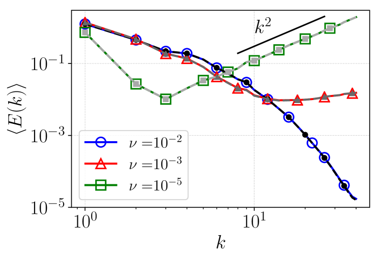
In Fig. 1 we present a first comparison between and by looking at at changing and for fixed spatial resolution, . Here, we have omitted in the label and for simplicity and the same will be done in what follows whenever it does not lead to ambiguities. All regimes can be accessed as the viscosity is varied, and in terms of the average energy spectrum, the and agree remarkably well. This will be further checked in the following with respect to the two conjectures. We anticipate that deviations will appear at scales beyond the Kolmogorov scale , which will be further explored later. Next we will deal with the two regimes separately.
III.3 Mean properties of
A rigorous (yet non trivial, see below) consequence of both conjectures is the relation
| (14) |
which holds when Eq. (10) holds. In Fig. 2(a) we validate Eq. (14). The errors are calculated by where is the standard deviation, the non-dimensional autocorrelation time, and the ensemble size.
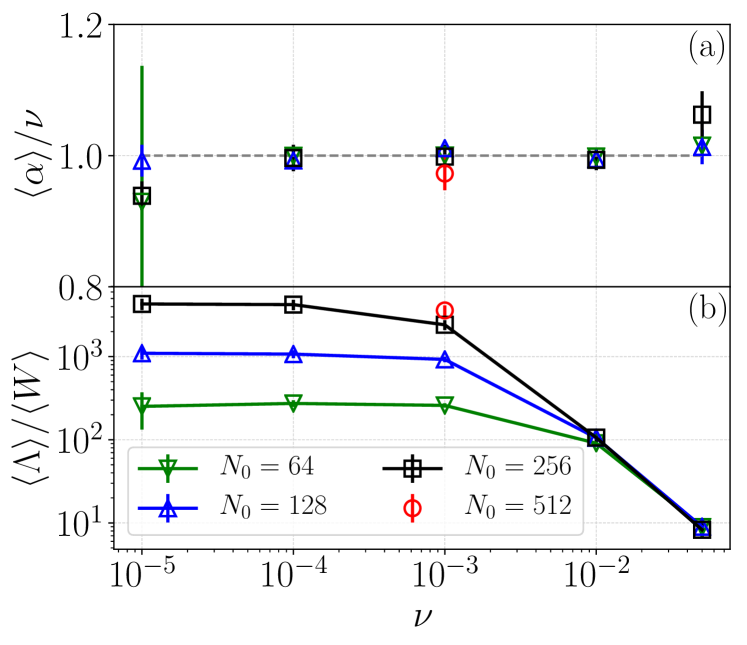
Figure 2(a) provides a consistency check, which looks at first not entirely obvious because is not a local observable; see the definition given in Eq. (7). Yet, if the conjectures and condition (10) hold, it must be true that the ensemble average of is equal to the viscosity. This follows from the balance between energy input and output in steady state conditions that hold both for and :
|
|
(15) |
Under the equivalence condition , the value must be the same in and , because is a local observable. Hence, the relation imposes the equality of the averages for the and systems, which, in turn, implies the non trivial relation (14). We remark that, as can be measured also in , we can also check its statistics. We observe that in all statistical regimes, which is nontrivial because it is not a consequence of the equivalence conjecture because is not a local observable. Although the distributions of in both and are in all cases peaked around , as well as the mean values of both and are approximately equal to , their tails are different in the hydrodynamic regime, but become almost identical in the quasithermalized regime (see Sec. IV.2).
Since is a sum of the forcing contribution and of the internal nonlinear contribution (8), it is interesting to remark that, on average, the non linear term dominates the forcing one as shown in Fig. 2(b), where the ratio versus is plotted. The ratio increases linearly as decreases in the hydrodynamic regime, before it approaches a (large) constant depending on in the quasithermalized regime. Thus, on average the internal nonlinear exchanges dominate over the forcing for the dynamics, introducing a non-local (in scale) coupling among all modes and making the validity of conjecture 2 even less trivial.
III.4 Test of conjecture 1: Quasithermalized regime
In this section we address the validity of conjecture 1 for 3D NSE. We remark that it has been confirmed in simpler dynamical systems in (18; 20; 21; 22). conjecture 1 applies when we consider decreasing values of at fixed , which leads to the quasithermalized regime. In terms of observables, we consider the single mode kinetic energy, and the energy spectrum, (13) which will be presented separately.
III.4.1 Single mode energy
We consider the probability distribution function (PDF) of the energy of a certain mode . In Fig. 3 we test this for a chosen type of modes, , with , and we see a very good agreement between the two ensembles, where the output of is shown in red straight lines, while black dashed lines are used for the simulations. In our analysis we have considered several different types of modes, i.e.,permutations of , and , with and 2, or 7, or 9 (the latter integers were randomly chosen). The PDFs approximately follow a distribution.
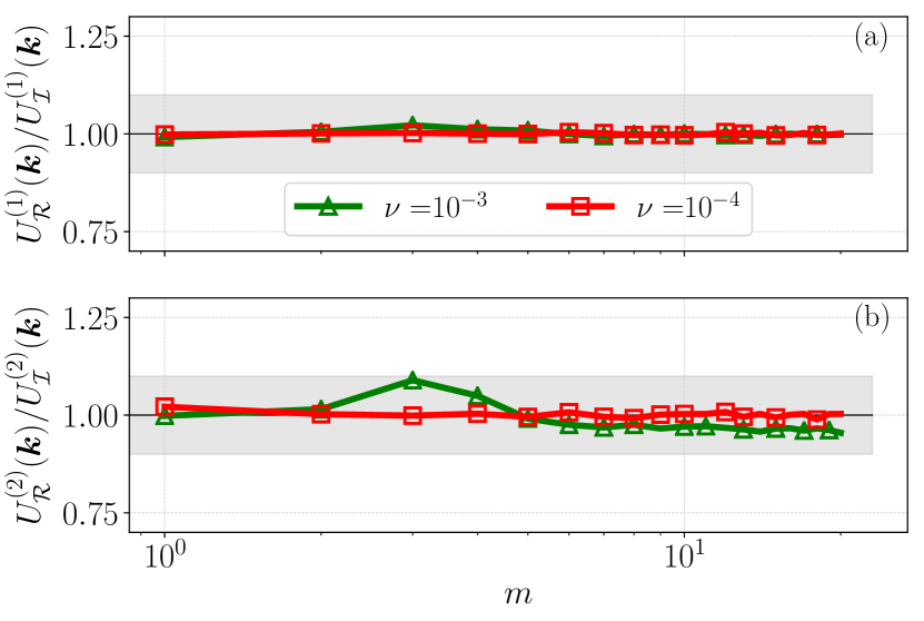
To further quantify the comparison between and , we study the statistical properties of the ensembles of by computing the mean , and the standard deviation of the time series for each measured mode . An indication of equivalence is when the ratios of such quantities are close to 1. In Fig. 4 we present the ratios of the mean (a) and the ratios of the standard deviation (b). To increase statistical accuracy, we further average the resulting ratios of the different types of modes considered here at each , corresponding to the same shells . As shown in Fig. 4, by fixing while decreasing , conjecture 1 holds well in the case of single mode kinetic energy, which is a prototypical local observable, for the run (R). Note that the run (R) belongs to the crossover regime, hence outside the domain of validity of conjecture 1, leading to some small deviations from 1 in Fig. 4(b). As a confidence interval, we introduce on qualitative grounds a 10% deviation from 1, displayed as a gray band.
III.4.2 Energy spectrum
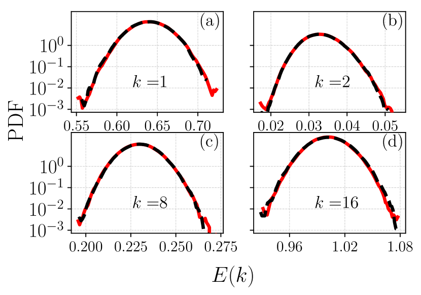
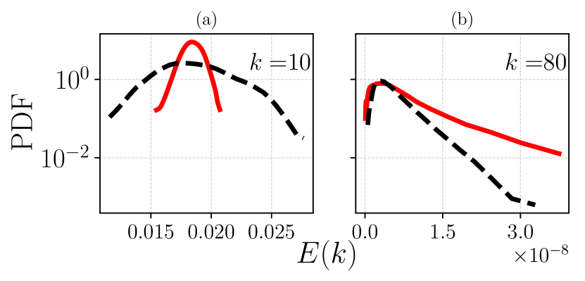
Subsequently, we study the energy spectrum, which has been briefly presented in Fig. 1. In Fig. 5 we show the PDF of kinetic energy for different shells for the case and (R). We notice that the statistics of and are almost identical and are approximately Gaussian as previously observed in (35); deviation from Gaussianity are nonetheless present for .
In Fig. 6 we summarize the equivalence between the two ensembles by plotting the same of Fig. 4 but for the spectral properties at changing and at fixed . Accordingly, we define the mean , and the standard deviation of the time series for each shell . As one can see, conjecture 1 is well verified at decreasing and for any . Notice in Fig. 6(b) that the standard deviation ratios for (green line-points) are different from 1 except for very small values of . This is to be expected, as this case (R) belongs to the crossover regime, hence outside the domain of validity of conjecture 1. Interestingly, for the same parameters, , , the single mode standard deviation ratios are close to 1; see the green line in Fig. 4(b). This reflects the higher complexity of the energy spectrum, resulting from the presence of correlations among Fourier modes. All the above confirm the validity of conjecture 1.
III.5 Test of conjecture 2: Hydrodynamic regime
We now present our numerical tests of conjecture 2, which applies at fixed when is large, corresponding to the hydrodynamic regime. We follow a systematic approach by first keeping the value of fixed, and then progressively increase the value of . We then repeat this protocol for different values of . Again, we consider the single mode kinetic energy and the energy spectrum.
III.5.1 Single mode energy
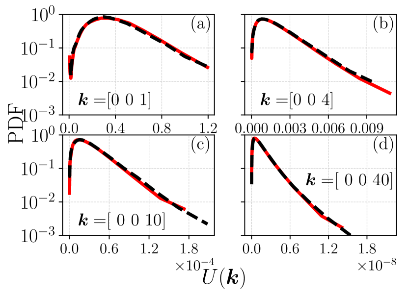
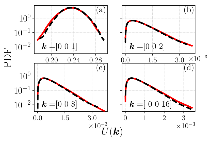
In Fig. 7 we fix , (R) and compare the PDF of single mode kinetic energy, shifted to their mean, for the modes , 4, 10, 40 between and . The agreement between the two ensembles is compelling.
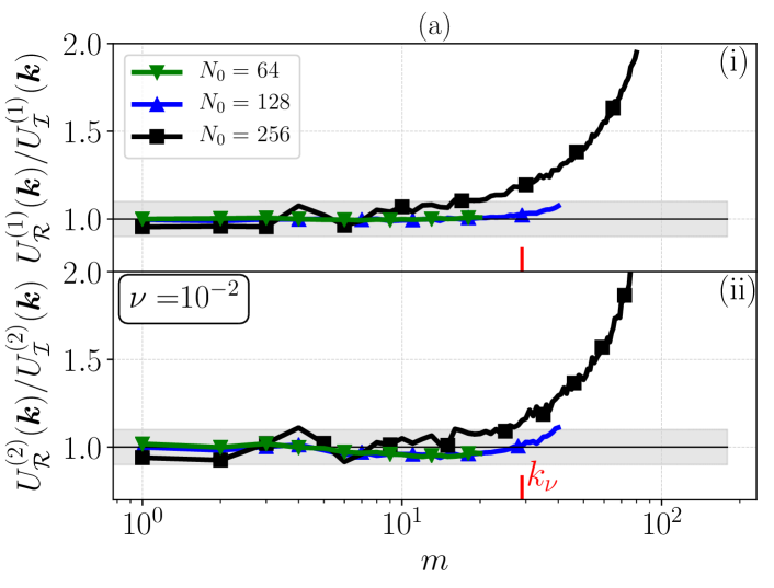
A further analysis can be seen in Fig. 8 where all mean and standard deviation ratios of the time series have been collected for (a) and (b) for different values of and . In Fig. 8, for scales beyond the Kolmogorov scale (indicated by the red tick), we observe a disagreement between and .
Therefore, one could argue that, within the numerical set-up we have investigated in this work, is an approximate upper bound (in the sense of order of magnitude) for the maximum wave number for which the conjecture 2 applies; or as stated after Eq. (12), , both when considering , and . The observed difference between the and ensembles for is further confirmed for all our well-resolved runs in the hydrodynamic regime. On the other hand, in the cross-over regime, i.e., here for R in Fig. 8(a) and R, R in Fig. 8(b), the agreement for single mode statistics of the two ensembles, although not expected by conjecture 2, is satisfactory.
III.5.2 Energy spectrum
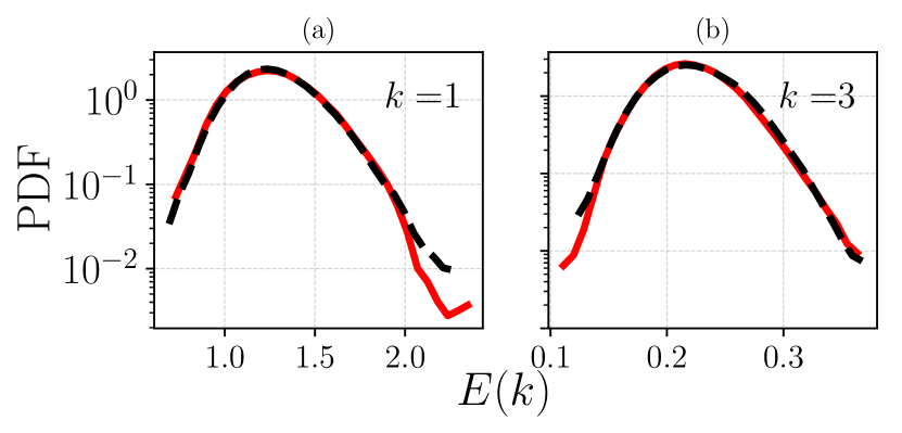
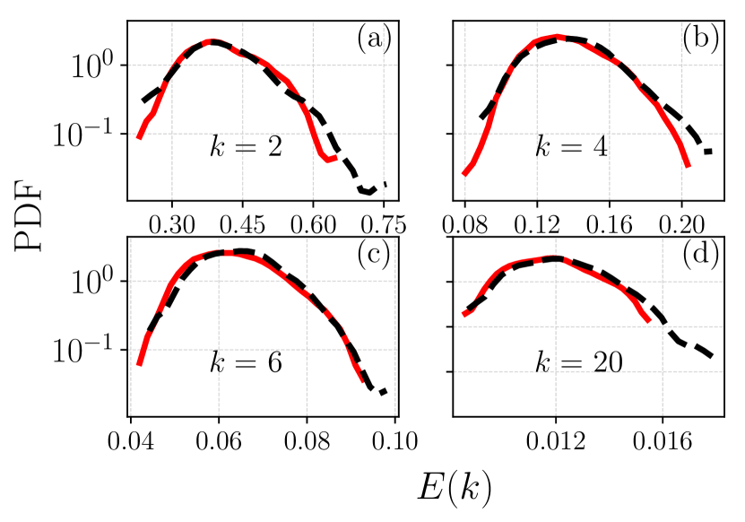
With respect to the energy spectrum at the hydrodynamic regime, we first present the distributions at low . In Fig. 9 we plot the PDF of energy spectra at and 3 for at (R7) and we observe a very good agreement between (red line) and (black dashed line). Then, in Fig. 10 the same are shown for a larger range of , i.e., 2, 4, 6, 20 and a smaller viscosity, at (R16), which is the only fully resolved run at . Again, the agreement between the two ensembles is remarkable, and slight disagreement at the tails is likely due to statistical accuracy.
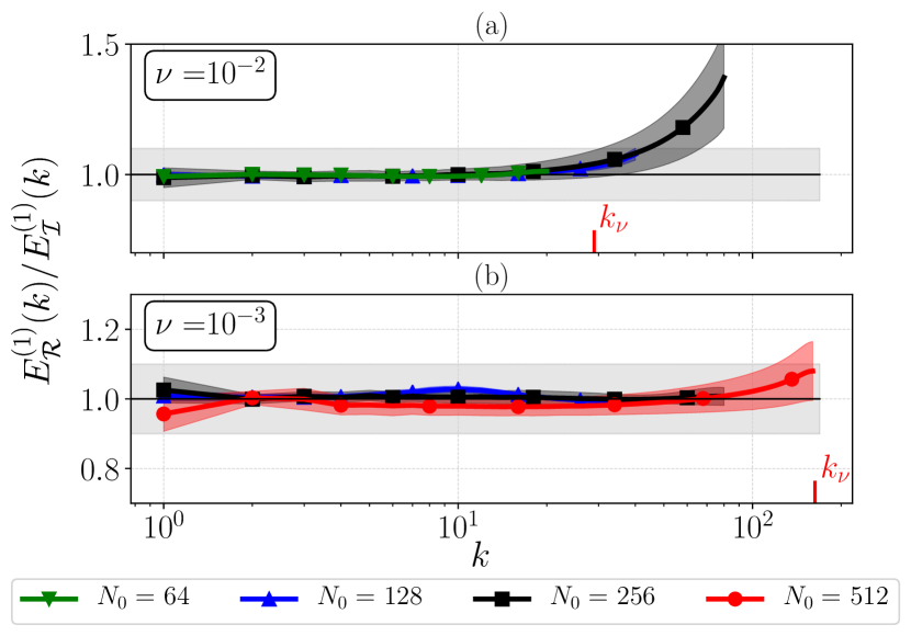
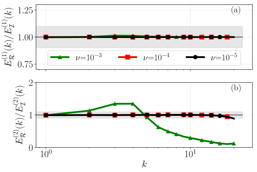
In Fig. 11 we collect the mean energy spectrum at different . We test the conjecture 2 by quantifying the agreement between and through the ratio , while fixing , at changing . A deviation from 1 would indicate disagreement with respect to this observable. In Fig. 11(a) at we remark that (R3) is slightly under-resolved (not well developed fall-off region in the spectrum), but still follows the same trend as the rest of the well resolved simulations at increasing . Deviations occur for when the ratio of is considered. In Fig. 11(b) we show the results for , where for all cases the ratio is close to 1 up until , which is close to the cut-off of . Also in (b), the ratio of the under-resolved runs ( and ) stays unity for all .
III.5.3 Empirical determination of the locality cutoff
So far, the cases we have studied reveal a very good agreement between and for the quasithermalized regime (see Sec. III.4), which confirms conjecture 1, and full agreement for the hydrodynamic regime for when considering , , and . In accordance with the definition of conjecture 2, we recall that a scale can be defined such that observables depending on with can be considered “local”, thus determining the domain of validity of conjecture 2. Furthermore, conjecture 2 states that with as . We state now that and accordingly , can differ when considering different observables for testing the equivalence. Indeed, for , , and we concluded that .
Next, we look at the statistics of energy spectrum at larger . In Fig. 12 we show two examples where disagreement is observed in the case of . Taking (R12) we show in Fig. 12(a) the PDF of at , for which the ratios [see Fig. 11(a)], but . In Fig. 12(b) we choose a larger than the Kolmogorov scale, i.e., , and both ratios of mean and standard deviation between and are not equal to 1.
In Fig. 13 we quantify the behavior of the standard deviation of each ensemble, by considering their ratio for all . conjecture 2 is tested for fixed , (a) and (b) at increasing . Starting from there is initially agreement between and but we observe that departs from unity at a smaller than , which is also smaller than . Notice that in (a) the runs with and are fully resolved and belong to the hydrodynamic regime, and although the runs at are slightly under-resolved, it follows the same trend with the rest. Moreover, once the cut-off is larger than by a sufficient margin, further increases in do not change the features of the ratio curves, both for and . Instead, in (b) only the case is fully resolved, and although for all [see Fig. 11(b)] the standard deviation ratios differ when changing . This occurs because and are under-resolved at , and belong to the crossover regime (hence outside the validity of conjecture 2), but are still displayed to show the transition from crossover to hydrodynamic regime, and how the agreement improves in that case.
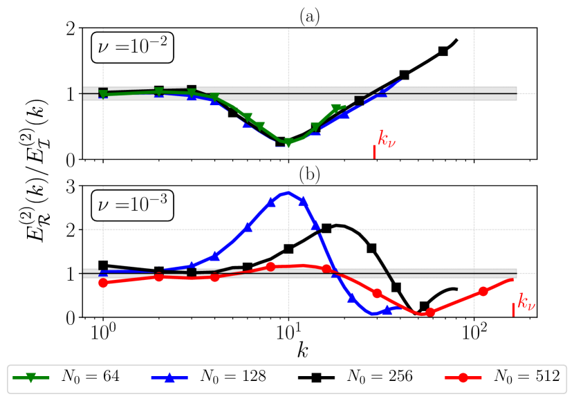
To be more specific about the deviation from 1 with respect to Fig. 13, for (a) at it appears that . Instead, from Fig. 13(b) at it appears . The fact that increases at decreasing , with sufficiently large , is foreseen by conjecture 2, and confirmed here. In other words, equivalence between and holds for a larger range of , as decreases, when the testing criterion is the shape of the distributions of , or similarly the standard deviation of it, .
Note that the location of the minimum of in Fig. 13 shifts with changing for well-resolved simulations. It actually corresponds to the end of the inertial range, and it is related to the chosen observable that is kept fixed in . Since here we chose the enstrophy , which is dominated by the small scales, i.e., large , the constraint actually suppresses the fluctuations of , for those around the end of the inertial range; see also Fig. 12(a). A similar result was observed in (21).
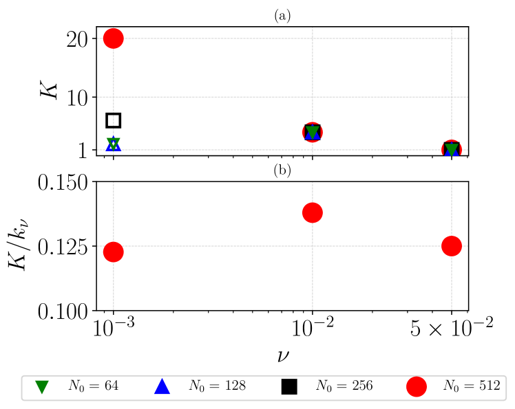
The resulting values of as extracted from second order moments of the energy spectrum, , are gathered in Fig. 14(a) for runs in the mixed hydrodynamic-crossover regime. Both at and the runs are in the hydrodynamic regime, while at only (R16) is well resolved, for which we notice that is maximum. In Fig. 14(b) we show that the empirically determined does scale proportionally to , indicating that the range of scales where conjecture 2 holds is increasing with the Reynolds number, i.e. supporting the statements that conjecture 2 is uniformly valid in a sub-set of the inertial range for all turbulent intensities.
From Figs. 7–12, as well as Fig. 14(b), and with reference to conjecture 2 it appears that within the case studied here we have the following:
-
•
when considering , , and for the Equivalence test, and
-
•
when considering .
All the above confirm the validity of conjecture 2 up to some wave number .
IV Properties of the Reversible Navier-Stokes equations
In the previous section we have established the domain of validity of conjecture 2, and hence the equivalence of the two non-equilibrium ensembles, using a dimensionless scale-by-scale comparison for different local observable, based on single Fourier modes energy or shell energy (see Figs. 6, 8, 11, and 13). We have shown that the equivalence holds up to some wave number . Similar results are shown when comparing the whole probability distribution function of the same quantities. These results extend and clarify the recent investigations (27; 28) where the equivalence was tested on the basis of the energy spectrum or on the global scaling properties of high order moments of the velocity increments in the inertial range only.
Let us remark that the property valid in that is a finite non-zero constant of motion has obvious implications on the sequence of solutions and for the Leray’s solutions (36; 37), which are their weak limits as . Perhaps the most remarkable is an a priori upper bound on which can be proven (see Appendix A) to satisfy, for any solution and any , the condition:
| (16) |
A second interesting and potentially very important remark on the evolution is that if for all large enough there were such that also: , with probability in the stationary state, then, it is possible to conclude that the attractor consists of with derivatives of all orders bounded uniformly in , i.e., on the attractor the fields are uniformly smooth. This is an immediate consequence of the autoregularization results, (see Proposition 5, Sec. 3.2, in (38), and (39)), and of the constancy of the enstrophy , as shown in the Appendix B. Positivity of the lower bound on is expected at large viscosity i.e., small .
Note also that by combining the aforementioned bound of Eq. (16), as proposed in the literature, with the fact that the dissipation in has a positive limit as should indicate, (see (40, p.306)), that the upper bound on is , which puts a limit to the fluctuations of (which by the conjecture is on average equal to ; see also Sec. III.3). Furthermore the upper bound (16) suggests that the transport contribution to (i.e., ) might dominate over the second term (i.e., the forcing contribution ), as confirmed in Fig. 2(b).
IV.1 Numerical results about the sign of in
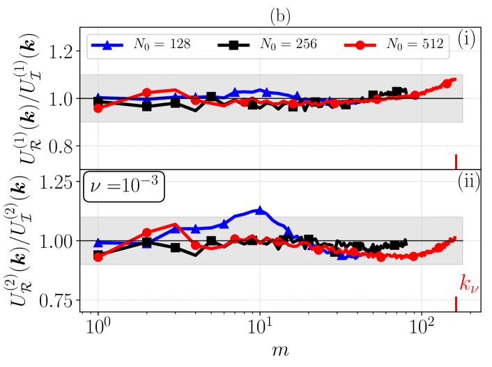
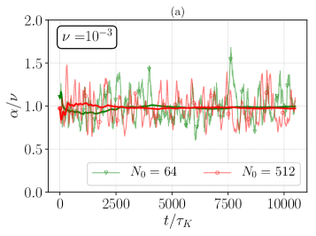
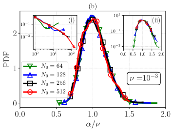
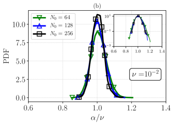
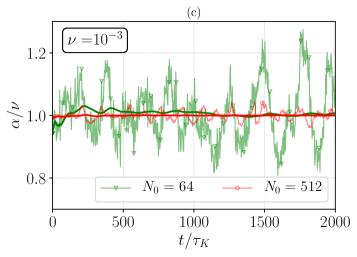
In this section we inspect the statistics of the fluctuations of for , in order to assess the probability to observe negative values at varying the control parameters. In Fig. 15(a) we show in light colors the temporal evolution of , and in solid colors its running average, performed as for at and (green - R3 and red - R16, respectively). The presented time window, which is scaled by the Kolmogorov time , is the maximum achieved for the run with (R16), while for R3 this is only about 1% of its total temporal extend. Then, in Fig. 15(b) the PDFs of are presented for , 128, 256, and 512 at . Notably, all PDFs agree, even though at only is fully resolved, belonging therefore to the hydrodynamic regime, while the other simulations belong to the crossover regime. The inset plots (i) and (ii) are respectively the energy spectrum and the PDF in semilogarithmic scale.
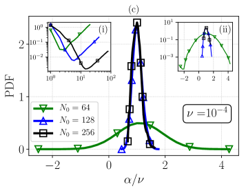
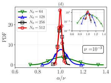
In Fig. 15(c) we show the same of Fig. 15(b) but at lower viscosity, , where the data set at (R4) is in the quasithermalized regime, while the other runs are in the crossover regime. As one can see, except for the case of the quasithermalized regime, in all other simulations we do not observe negative values of within our statistical sample.
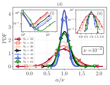
Additionally, in Fig. 15(d) we perform a detailed study at fixed and low resolution, in order to observe when, and how the transition to the occurrence of frequent negative values of takes place. Starting from and gradually decreasing , we observe that the PDF of first turn from non-Gaussian to quasi-Gaussian, while becoming narrower (see and ), before starting to widen (see ), until occurrence of events appears (see ). The rapid change in the left tail of the PDF at changing suggests that in order to further substantiate the asymptotic probability to observe negative values, when is large and in the presence of intermediate or hydrodynamical regimes, one would need statistical samples significantly (exponentially) larger than those we could generate here, which is by far out of the scope of this paper and probably out of reach given the available computational power. This result is in agreement with some previous observations made in the context of a reduced model of turbulence (21).
In (28) negative values of are observed in an reversible ensemble at and Taylor-based Reynolds number Re. Indeed, such results are somewhat puzzling and are not expected on the basis of our data. We do not expect to be able to observe at such large and such Reynolds number by extrapolating from our results for the fully resolved hydrodynamical regime (see Sec. IV.2 below).
IV.2 Numerical results about the sign of in
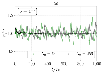
Interestingly enough, is an observable that can be measured also in the ensemble, by computing Eq. (7). In Fig. 16 we present the cases for two viscosities, [(a) and (b)] and [(c) and (d)]. In Figs. 16(a), 16(c) we show the time series of for a time window scaled by the Kolmogorov time scale , and in Figs. 16(b), 16(d) the corresponding PDF for different different resolutions .
First, from Figs. 16(a)–16(c) we note that also in the non-trivial result holds (see also Sec. III.3). On the other hand, from panels Figs. 16(b)–16(d) we observe some different behavior from the corresponding PDF of the ensemble in particular for the case of . In the latter case the high wave number range starts to depart from the hydrodynamic regimes and probably has a direct impact on the fluctuations of .
V Conclusions
We present a detailed numerical study of the 3D reversible Navier-Stokes equation [see Eq. (7)] obtained by imposing the conservation of enstrophy via a thermostat, and compare our results with the output obtained from the corresponding [see Eq. (3)] standard irreversible NSE case. We investigate two conjectures concerning the equivalence of the two ensembles. These conjectures, which had been previously presented in (2; 26), pertain to two limiting conditions. The first equivalence is studied by keeping the flow evolving on a finite set of modes, and by decreasing the viscosity of the irreversible system or, equivalently, increasing the total enstrophy of the reversible one. In this limit, which leads to the regime that we have dubbed quasithermalized in the sense of (32), the equivalence between the two ensembles is more and more accurate with decreasing for any fixed and for all scales, thereby confirming conjecture 1.
We emphasize that conjecture 2, which is the most relevant to the physics of turbulence, had never been tested in 3D Navier-Stokes in such a detail and rigor, and only partially in 2D Navier-Stokes. In particular, opposed to what was presented in (28), here we have studied the limit of larger and larger values of while keeping a fixed value for the viscosity, and then explored the limit. In this regime we empirically observe that the equivalence between the two ensembles is restricted to “local” observables having support in a region of the Fourier space restricted by a typical wave number , where is smaller than, but proportional to, . The latter observation has been made possible by extending the class of observable studied in (28) to high order moments of the Fourier energy content and to its whole probability distribution function. Our results are consistent against changes in and by decreasing the time discretization at least as far as we could test within our numerical capacities. The inertial-range equivalence between the two ensembles in the hydrodynamic limit is a further important confirmation of the robustness and universality of Navier-Stokes equations against changing of the dissipative mechanisms, at least concerning wave numbers smaller than . This is particularly non-trivial as the dissipative term of is highly nonlinear and non-local.
From our numerical results the prefactor entering in conjecture 2 is close to a constant or depending on the observable (see discussion in the end of Sec. III.5.3) and independently of . The question of the scaling in the limit remains an important open question that will require more numerical studies.
Note that, in Remark 4 of Sec. II.3, we mentioned a stronger version of conjecture 2, presented in (2; 26), where for all . Our results here make it appear doubtful that such conjecture could hold in such a strong sense. However, a study for a different fixed observable (instead of the enstrophy ), of the time scale, of the larger values , and of the integration precision necessary to reveal the dependence of , or even for all , may be necessary to reach a firm conclusion.
Furthermore, we have presented a numerical empirical study of the PDF of the fluctuating viscosity for the reversible case, showing the existence of a trend towards less and less probable negative events by increasing the Reynolds in the hydrodynamical regime, similarly to what had been observed in a reversible shell model (21). The problem of the sign of is related to that of the divergence of the phase-space contraction rate (26) and the problem of measuring the large deviations of is extremely delicate due to the fact that negative events are expected to happen with extremely small probability. We remark that, a recently published paper has presented results on the probability of observing negative values of (see Fig. 4 of (28)) that are in contrast with what has been reported for the hydrodynamical limit ( first) in this work. In particular, in (28) a transition in the shape of the PDF is observed for large numerical grids showing a non negligible probability to have negative events.
Finally, by studying the average of for the , we have shown that equivalence can also hold for a non local observable, which is a non trivial application of the conjectures. So, it would be natural to test whether equivalence might be extended to other important non local observables. For instance, the Lyapunov exponents, as done in a simpler model in (20), and in 2D NSE, (2; 24), where equivalence of the local Lyapunov spectra 222obtained from the Jacobian matrix, formally , by averaging over time the spectrum , , …, of the symmetric part of . is observed in several cases, in spite of its non local nature. Further numerical investigations by increasing both the cut-off , and the runs duration would be extremely useful to better elucidate the equivalence between the two ensembles in the asymptotic limit when first and later, the so called fully developed turbulence.
Acknowledgements.
This work was supported by the European Research Council (ERC) under the European Union’s Horizon 2020 research and innovation programme (Grant Agreement No. 882340). V.L. acknowledges the support received from the EPSRC Project No. EP/T018178/1 and from the EU Horizon 2020 project TiPES (Grant No. 820970). GM is grateful to Fabio Bonaccorso, Michele Buzzicotti and Mateo Lulli for useful discussions. This work has benefited from computational resources provided by the INFN-CINECA high performance computing facilities, by the NewTURB academic cluster at the University of Rome “Tor Vergata”, and, to a smaller extent, from INFN-FARM cluster at University of Rome “La Sapienza”.Appendix A Bound on
We recall Eq. (4), for which it is well known, that it leads to the a priori bounds
|
|
(17) |
satisfied (for all ) by the solution in terms of the square norms and , see for instance Proposition 1, Sec.3.2 in (38). There is no problem about the forcing term in Eq. (7) as Eq. (17) implies, if , a bound on it: . The other term has in the numerator which is bounded via the Hölder inequality with exponents by
| (18) |
and the three factors can be bounded via Sobolev’s inequality (41; 37): if then
|
|
(19) |
where is a sphere of radius and the integrals are performed with respect to . The is a suitable constant. The second term of the right hand side can be omitted if has zero average over .
Therefore in the above case, where do have zero average, choose , ; calling and , it is:
|
|
(20) |
so that
|
|
(21) |
and is thus bounded, for any solution and any , by a constant: .
Appendix B Reversible Navier-Stokes global smoothness
Let and suppose that the initial data and satisfy for all (recall that we consider only initial data and force with a finite number, , of modes, for simplicity). Let ; then .
Following, for instance (38), we can write , where is the non-linear term of the NSE. Therefore, the sum of the first and last term can be bounded by while the integral is bounded by
|
|
(22) |
so that adding the two bounds: for a suitable . Therefore, again, can be bounded by adding and a bound on
|
|
(23) |
A bound on the latter integral is obtained via the Schwartz inequality and the remark that implies , and
|
|
(24) |
where has been changed to just to make clear that summing over allows using the Schwartz inequality. Hence integration over , as in Eq. (22), yields
| (25) |
Thus if is finite the bound , Eq. (22), can be improved into . Iterating a autoregularization phenomenon sets in and
| (26) |
so that is a -functions and all its derivatives can be bounded in terms of the enstrophy , uniformly in . See Sec. 3.3 in (38) for related results on the classic autoregularization.
| R | R | R | R | R | |
| 1.015(7) | 0.999(3) | 1.000(4) | 1.000(8) | 0.93(20) | |
| 0.998(2) | 0.999(1) | 0.999(1) | 1.000(1) | 1.01(2) | |
| 1.22(1) | 1.30(1) | 1.46(1) | 2.92(1) | 7.00(1) | |
| Re | 43 | 185 | 1705 | ||
| Reλ | 30 | 77 | 300 | – | – |
| 0.74 | 0.72 | 0.76 | 0.66 | 0.39 | |
| 8 | 29 | 165 | – | – | |
| 1.23 | 0.59 | 0.21 | – | – | |
| 1.77 | 1.43 | 1.16 | 0.27 | 0.17 | |
| 8300 |
| R | R | R | R | R | |
| 1.01(3) | 0.995(5) | 1.011(6) | 0.99(1) | 0.99(2) | |
| 1.008(2) | 0.998(1) | 0.996(2) | 0.999(2) | 1.027(1) | |
| 1.22(4) | 1.29(3) | 1.36(3) | 1.88(4) | 4.61(1) | |
| Re | 43 | 183 | 1850 | ||
| Reλ | 30 | 76 | 267 | 1570 | – |
| 0.75 | 0.71 | 0.73 | 0.76 | 0.68 | |
| 8 | 29 | 164 | 932 | – | |
| 1.22 | 0.59 | 0.20 | 0.08 | – | |
| 1.78 | 1.42 | 1.36 | 0.72 | 0.13 | |
| 760 | 4690 | 4950 |
| R | R | R | R | R | |
| 1.06(4) | 0.99(2) | 1.00(2) | 1.00(2) | 0.94(2) | |
| 1.008(2) | 1.008(1) | 1.008(2) | 1.019(2) | 1.034(2) | |
| 1.251.21 | 1.29(5) | 1.35(5) | 1.46(5) | 2.70(6) | |
| Re | 44 | 184 | 1800 | ||
| Reλ | 31 | 76 | 260 | 973 | – |
| 0.780.73 | 0.71 | 0.73 | 0.71 | 0.740.79 | |
| 8 | 29 | 164 | 919 | – | |
| 1.261.22 | 0.59 | 0.19 | 0.06 | – | |
| 1.80 | 1.42 | 1.33 | 1.18 | 0.36 | |
| 374 | 680 | 760 | 800 | 3950 |
| R | Re | Reλ | ||||
|---|---|---|---|---|---|---|
| 0.97(3) | 0.997(2) | 1.35(5) | 1800 | 260 | ||
| 0.71(7) | 163 | 0.19 | 1.35 | 400 |
Appendix C Numerical parameters
Table 1 summarizes the values of various observables corresponding to the runs with different kinematic viscosities and cut-offs. The parentheses present the statistical error of the last digit in a given value. We define the following: physical length of the container , root-mean-square velocity , averaged rate of energy dissipation , is the Kolmogorov scale, Taylor length , integral length (see Eq. 13), Taylor-Reynolds number , Reynolds number , large-eddy turnover time .
We present the final ratio, which is an abbreviation for . Ideally, this should be 1, and it is indeed unity when we start the simulation based on the ensemble average from . But for almost all runs, we increased the statistics of , which eventually improved . Therefore the ratio gives an estimate of the quality of each collection of runs with respect to the collection for a particular . A significant discrepancy would also explain possible discrepancies in and accordingly other ratios of observables.
The ratio , where is the total length of the simulation in physical units, is essentially an indicator of the statistical significance of the generated ensemble. Empty entries (filled with a “–”) are met in cases at the quasithermalized regime for particular observables of which the definitions are relevant in the hydrodynamic regime (e.g. ).
An interesting fact about Table 1 is that the averaged values for each entry turn out to be the same on average, up to statistical errors, for both and . Showing one value, implies that is it the same for and at the particular and . When the averages are not the same within statistical errors we show both estimates in the form . This happened in the case of in two cases, namely R and R, see e.g. . For R we attribute this to poor statistics, notice , which is the lowest, and for R we attribute to a poor estimation of , notice , which is the highest.
References
- Gallavotti (2014) G. Gallavotti, Nonequilibrium and irreversibility, Theoretical and Mathematical Physics (Springer-Verlag, 2014).
- Gallavotti (2020a) G. Gallavotti, Journal of Statistical Physics 180, 172 (2020a).
- Frisch (1995) U. Frisch, Turbulence: The Legacy of A. N. Kolmogorov (Cambridge University Press, 1995).
- Pope (2000) S. B. Pope, Turbulent Flows (Cambridge University Press, 2000).
- Salmon (1998) R. Salmon, Lectures on geophysical fluid dynamics (Oxford University Press, 1998).
- Alexakis and Biferale (2018) A. Alexakis and L. Biferale, Physics Reports 767, 1 (2018).
- Frisch et al. (2008) U. Frisch, S. Kurien, R. Pandit, W. Pauls, S. S. Ray, A. Wirth, and J.-Z. Zhu, Phys. Rev. Lett. 101, 144501 (2008).
- Cercignani (1988) C. Cercignani, “The boltzmann equation,” in The Boltzmann Equation and Its Applications (Springer New York, New York, NY, 1988) pp. 40–103.
- Zwanzig (2001) R. Zwanzig, Nonequilibrium statistical mechanics (Oxford university press, 2001).
- Onsager and Machlup (1953) L. Onsager and S. Machlup, Phys. Rev. 91, 1505 (1953).
- Bertini et al. (2002) L. Bertini, A. De Sole, D. Gabrielli, G. Jona-Lasinio, and C. Landim, Journal of Statistical Physics 107, 635 (2002).
- Ruelle (1999) D. Ruelle, Statistical Mechanics (CO-PUBLISHED WITH IMPERIAL COLLEGE PRESS, 1999) https://www.worldscientific.com/doi/pdf/10.1142/4090 .
- Touchette (2015) H. Touchette, Journal of Statistical Physics 159, 987 (2015).
- Evans and Morriss (1990) D. J. Evans and G. P. Morriss, Statistical Mechanics of Nonequilibrium Fluids (Academic Press, New-York, 1990).
- She and Jackson (1993) Z. She and E. Jackson, Physical Review Letters 70, 1255 (1993).
- Gallavotti (1996) G. Gallavotti, Physics Letters A 223, 91 (1996).
- Gallavotti (1997) G. Gallavotti, Physica D 105, 163 (1997).
- Gallavotti et al. (2004) G. Gallavotti, L. Rondoni, and E. Segre, Physica D 187, 358 (2004).
- Gallavotti (2020b) G. Gallavotti, European Physics Journal, E 43:37 (2020b), 10.1140/epje/i2020-11961-0.
- Gallavotti and Lucarini (2014) G. Gallavotti and V. Lucarini, Journal of Statistical Physics 156, 1027 (2014).
- Biferale et al. (2018) L. Biferale, M. Cencini, M. D. Pietro, G. Gallavotti, and V. Lucarini, Physical Review E 98, 012201 (2018).
- Pietro et al. (2018) M. D. Pietro, L. Biferale, G. Boffetta, and M. Cencini, The European Physical Journal E 41, 48 (2018).
- Seshasayanan et al. (2021) K. Seshasayanan, K. S. Eswaran, M. Maji, S. Ghosh, and V. Shukla, “Equivalence of nonequilibrium ensembles: Two-dimensional turbulence with a dual cascade,” (2021), arXiv:2112.12215 [physics.flu-dyn] .
- Gallavotti (2018) G. Gallavotti, European Physics Journal Special Topics 227, 217 (2018).
- Gallavotti (2019) G. Gallavotti, Springer Proceedings in Mathematics & Statistics 282, 569 (2019).
- Gallavotti (2021) G. Gallavotti, Journal of Statistical Physics 185 (2021), 10.1007/s10955-021-02830-1.
- Shukla et al. (2019) V. Shukla, B. Dubrulle, S. Nazarenko, G. Krstulovic, and S. Thalabard, Phys. Rev. E 100, 043104 (2019).
- Jaccod and Chibbaro (2021) A. Jaccod and S. Chibbaro, Phys. Rev. Lett. 127, 194501 (2021).
- Fefferman (2000) C. Fefferman, Existence & smoothness of the Navier–Stokes equation, The millennium prize problems (Clay Mathematics Institute, Cambridge, MA, 2000) pp. 57–67.
- Maxwell (2011) J. C. Maxwell, The Scientific Papers of James Clerk Maxwell, edited by W. D. Niven, Cambridge Library Collection - Physical Sciences, Vol. 2 (Cambridge University Press, 2011).
- Gallavotti (2006) G. Gallavotti, Chaos 16, 043114 (+6) (2006).
- Alexakis and Brachet (2020) A. Alexakis and M. Brachet, Journal of Fluid Mechanics 884, A33 (2020).
- Orszag (1971) S. A. Orszag, Journal of the Atmospheric sciences 28, 1074 (1971).
- Pekurovsky (2012) D. Pekurovsky, SIAM Journal on Scientific Computing 34, C192 (2012), https://doi.org/10.1137/11082748X .
- Brun and Pumir (2001) C. Brun and A. Pumir, Phys. Rev. E 63, 056313 (2001).
- Leray (1934) J. Leray, Acta Mathematica 63, 193 (1934).
- Caffarelli et al. (1982) L. Caffarelli, R. Kohn, and L. Nirenberg, Communications on Pure and Applied Mathematics 35, 771 (1982).
- Gallavotti (2005) G. Gallavotti, Foundations of Fluid Dynamics ((second printing) Springer Verlag, Berlin, 2005).
- J.Serrin (1962) J.Serrin, Archive for Rational Mechanics and Analysis 9, 187 (1962).
- Kraichnan (1975) R. H. Kraichnan, Advances in Mathematics 16, 305 (1975).
- Sobolev (1963) S. Sobolev, Applications of Functional analysis in Mathematical Physics, Translations of the American Mathematical Society, Vol. 7 (AMS, Providence, 1963).