Non-equilibrium phase transitions in active rank diffusions

The run-and-tumble particle (RTP), driven by telegraphic noise ML17 ; kac74 , is the simplest model of an active particle which mimics e.g. the motion of E. Coli bacteria Berg2004 ; TailleurCates . Interacting RTP’s, which exhibit remarkable collective effects, is a thriving area of research TailleurCates ; FM2012 ; soft ; CT2015 ; slowman ; slowman2 ; BG2021 ; SG2014 . One outstanding question is to characterize the non Gibbsian steady state reached at large time. Even in one dimension (1D), there are very few exact results, beyond two interacting RTP’s slowman ; slowman2 ; us_bound_state ; Maes_bound_state ; nonexistence ; MBE2019 ; KunduGap2020 ; LMS2019 , or for harmonic chains SinghChain2020 ; PutBerxVanderzande2019 . Recently, analytical results were obtained for some many-particle models on a 1D lattice with contact interactions Metson2022 ; MetsonLong ; Dandekar2020 ; Thom2011 , and for an active version of the Dyson Brownian motion in the continuum with logarithmic interactions TouzoDBM2023 .

An analytically tractable passive example is the Langevin dynamics of Brownian particles interacting via the linear Coulomb 1D potential. It is known as ranked diffusion since the force acting on each particle is proportional to its rank, i.e., the number of particles in front of it, minus the number behind. Introduced in finance and mathematics Banner ; Pitman , it is related to the statistical mechanics of the self-gravitating 1D gas Rybicki ; Sire (attractive case) and to the Jellium model (repulsive case, in presence of a confining potential) much studied at equilibrium Lenard ; Baxter ; Tellez ; Lewin ; SatyaJellium1 ; Chafai_edge ; Flack22 . Recently, a detailed description of the non-equilibrium dynamics was obtained PLDRankedDiffusion , using both a mapping to the delta Bose gas, solvable by the Bethe ansatz, as well as the Dean-Kawasaki approach Dean ; Kawa , which leads to a description of the density in terms of a noisy Burgers equation PLDRankedDiffusion . In the attractive case, the shock solutions of the Burgers equation correspond to macroscopic bound states, while in the repulsive case the system forms an expanding crystal at large time FlackRD .

In view of these results, it is natural to extend the model to the active case. In this Letter we study $N$ run-and-tumble particles (RTP) at positions $x_{i}(t)$ in $d=1$, interacting via the 1D Coulomb potential and evolving via the equation of motion

Here the $\xi_{i}(t)$ are unit independent white noises and the $\sigma_{i}(t)=\pm 1$ are independent telegraphic noises with rate $\gamma$. The particles can cross freely, i.e. there is no hard core repulsion, and by convention ${\rm sgn}(0)=0$. The case $\bar{\kappa}>0$ corresponds to attractive interactions and $\kappa=-\bar{\kappa}>0$ to repulsive ones. The RTP’s evolve in a common external potential $V(x)$. When $V(x)=0$ the center of mass $\bar{x}=\frac{1}{N}\sum_{i}x_{i}$ evolves as a sum of $N$ independent RTP’s with velocities $v_{0}/N$, hence it diffuses at large time as $\bar{x}\sim\sqrt{2D_{N}t}$ with $D_{N}=\frac{1}{N}(T+\frac{v_{0}^{2}}{2\gamma})$.

Until now this model was studied only for $N=2$, in the attractive case $\bar{\kappa}>0$, and for $V(x)=0$. It was shown us_bound_state that the PDF $P(z,t)$ of the relative coordinate $z=x_{1}-\bar{x}=\frac{x_{1}-x_{2}}{2}$ reaches a stationary limit $P(z)$ which describes a bound state. For $T>0$, $P(z)$ is the sum of three decaying exponentials. In the purely active limit $T=0$, some of these exponentials become delta functions, and it was found us_bound_state that for $\frac{v_{0}}{\bar{\kappa}}>\frac{1}{2}$

while for $\frac{v_{0}}{\bar{\kappa}}<\frac{1}{2}$ one has $P(z)=\delta(z)$, i.e all particles form a single cluster ($c_{2}=1$). Indeed since particles at the same position do not interact (${\rm sgn}(0)=0$), clusters tend to form when the interaction is strong enough. Obtaining the full stationary distribution for any number $N>2$ of particles would be very interesting, but is quite challenging PLDGS . Here we study the time dependent density fields $\rho_{\sigma}(x,t)$ with $\sigma=\pm 1$ and their even and odd components $\rho_{s}$ and $\rho_{d}$, defined as

An outstanding question is whether the delta peak in the density survives when $N$ increases. We first investigate this question numerically for finite $N$. Next, using the Dean-Kawasaki approach Dean ; Kawa , as in PLDRankedDiffusion for the passive case, and in TouzoDBM2023 for the active Dyson Brownian motion, we show that the density fields evolve according to two coupled stochastic non-linear equations. In the large $N$ limit these equations become deterministic and of the Burgers type. From them we obtain the exact solution for the $N$ particle stationary bound state. We also extend our results in the presence of an external linear potential both in the attractive and repulsive case. This leads to a rich phase diagram at $T=0$, with phases where the density is either smooth or contains shocks (i.e clusters) at various positions, as well as phases describing an active expanding crystal.

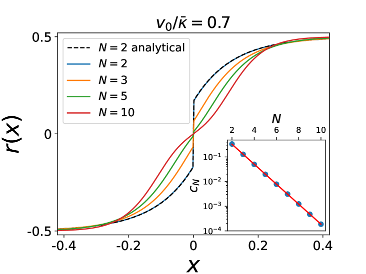
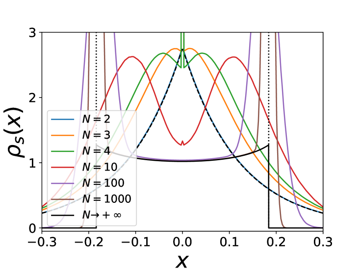
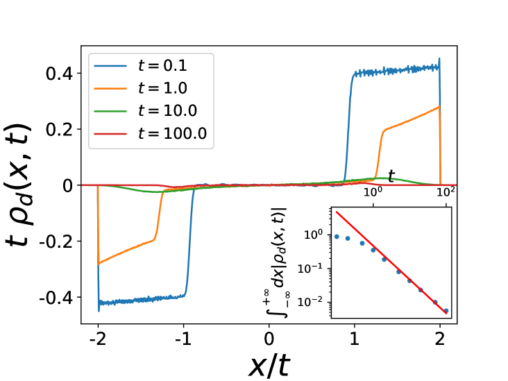
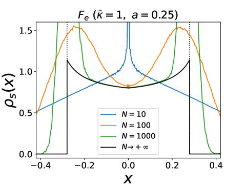
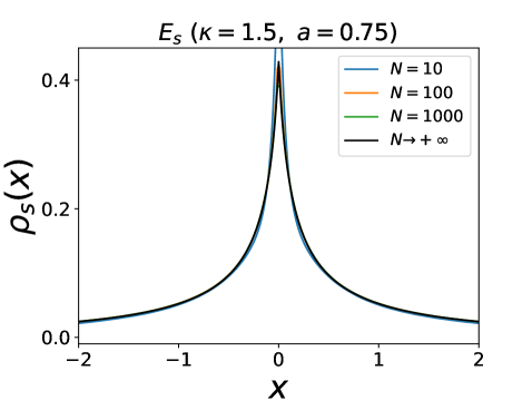
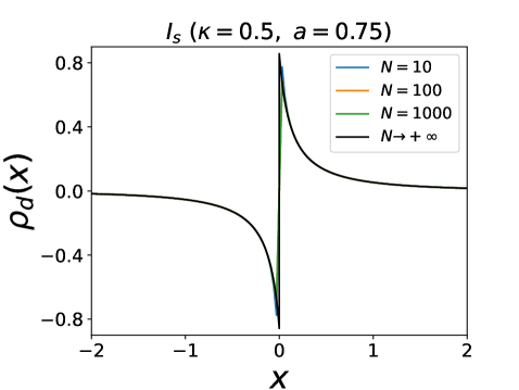
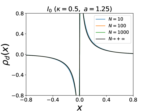
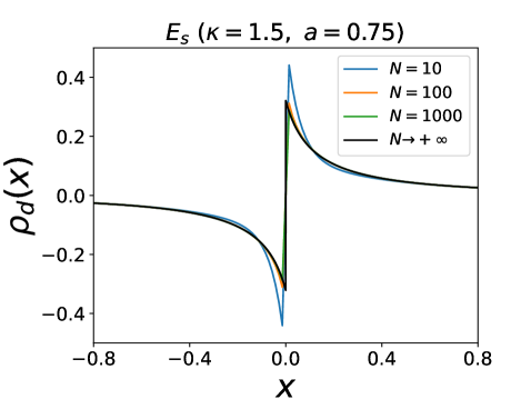
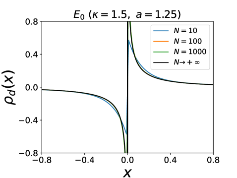
We have performed numerical simulations of Eq. (1) at $T=0$ for various numbers of particles $N$. In the attractive case with $V(x)=0$ we have measured the density of particles in the stationary state by performing time averages over a long time window. Here the density is measured in the reference frame of the instantaneous center of mass (this distinction becomes irrelevant at large $N$). The results are shown in Fig. 1. One finds that the delta function at $x=0$ in $\rho_{s}(x)$ persists for any finite $N$, with an amplitude $c_{N}$ which depends on $\frac{v_{0}}{\bar{\kappa}}$ and on $N$ (which is the only dimensionless parameter in that case). The first result is that for $\frac{v_{0}}{\bar{\kappa}}<1/2$ all particles are in a single cluster at $x=0$, i.e. $c_{N}=1$ for any $N$. Indeed, one can show that this configuration is stable. Denote $x_{+}$ (resp. $x_{-}$) the position of one of the rightmost (resp. leftmost) particles and $n_{+}$ (resp. $n_{-}$) the number of particles at the same location. One has

since $n_{+}+n_{-}\leq N$. Hence for $\frac{v_{0}}{\bar{\kappa}}<1/2$ the width of the support always decreases to $0$. For $\frac{v_{0}}{\bar{\kappa}}>1/2$ we find that the amplitude $c_{N}$ decreases with $\frac{v_{0}}{\bar{\kappa}}$ and decays exponentially in $N$.

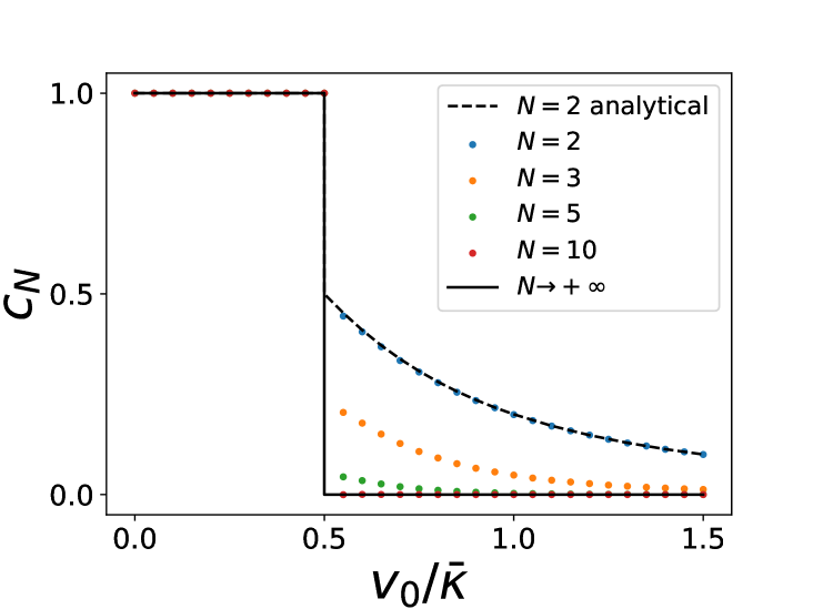
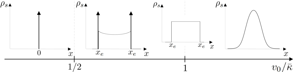
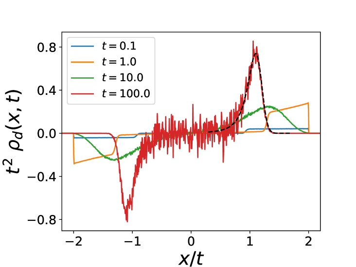
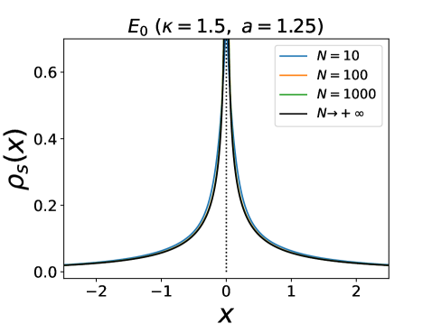
A remarkable feature, as we will see below, is that in the limit $N\to+\infty$ the delta peak at $x=0$ is absent for $\frac{v_{0}}{\bar{\kappa}}>1/2$, but for $v_{0}<\bar{\kappa}$ it is replaced by a pair of peaks at positions $\pm x_{e}$, which mark the edge of the (finite) support. A genuine phase transition occurs at $v_{0}=\bar{\kappa}$, as indicated in Fig. 2, beyond which the stationary density is smooth and the support extends to infinity. We now explain how these results are obtained.

Using the Dean-Kawasaki approach Dean ; Kawa , one can establish starting from (1) , as in PLDRankedDiffusion and TouzoDBM2023 , an exact stochastic evolution equation for the density fields, which takes the following form

where the $O(\frac{1}{\sqrt{N}})$ term represents the passive and active noises, see SM , and Sec. III A of TouzoDBM2023 . It is convenient to define, as in PLDRankedDiffusion , the rank fields

Focusing from now on on the large $N$ limit, and henceforth neglecting the noise terms in (Non-equilibrium phase transitions in active rank diffusions), one obtains from (Non-equilibrium phase transitions in active rank diffusions) and (8) two coupled deterministic differential equations (see SM )

These equations are valid both for the attractive and the repulsive case. Since $\rho_{s}(x,t)$ is positive and normalized to 1, $r(x,t)$ must be an increasing function with $r(\pm\infty,t)=\pm\frac{1}{2}$. One sees that $\partial_{t}s(+\infty,t)=-2\gamma s(+\infty,t)$, hence at large time $s(\pm\infty,t)=0$. In the passive case $v_{0}=0$ the first equation recovers Burger’s equation which describes usual rank diffusion PLDRankedDiffusion . One generally expects that in the diffusive limit $v_{0},\gamma\to+\infty$ with $T_{a}=\frac{v_{0}^{2}}{2\gamma}$ fixed, RTP’s behave as Brownian particles. This also holds here. Indeed, in (10) only two terms remain relevant, and one obtains $s\simeq-\frac{v_{0}}{2\gamma}\partial_{x}r$. Inserting in (9) the active term $-v_{0}\partial_{x}s(x,t)$ becomes $T_{a}\partial_{x}^{2}r(x,t)$, i.e. a thermal term.

We now turn to the analysis of the large time limit of these equations, starting with the case $V(x)=0$.

Attractive case. We set here $V(x)=0$. A stationary density then exists only in the attractive case $\bar{\kappa}>0$, which we now consider. To find this stationary density, we set the time derivatives to zero in (9), (10). The resulting equations are invariant by translation, hence we choose coordinates such that the center of mass $\bar{x}=\int dx\,x\,r^{\prime}(x)=0$. The first equation can be integrated leading to

In the absence of activity, $v_{0}=0$, the solution is that of standard rank diffusion, PLDRankedDiffusion

which for $T\to 0$ becomes a shock solution of Burgers equation, $r(x)=\frac{1}{2}{\rm sgn}(x)$, i.e a single delta peak in the density $\rho_{s}(x)=r^{\prime}(x)=\delta(x)$. At $T>0$ this shock solution acquires a finite width $x=O(T)$. One expects that for $v_{0}>0$ a similar rounding occurs at low $T$, not studied here. Instead, we focus directly on $T=0$ and $v_{0}>0$, i.e. pure telegraphic noise. In that case one must solve

keeping in mind the possibility that $r(x)$ may have jumps (see below). The first equation (13) can be integrated, leading to

Substituting in the second equation one obtains

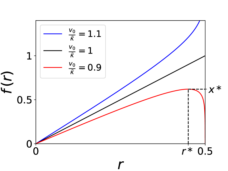
Since $|r(x)|\leq 1/2$ for all $x$, with $r(\pm\infty)=\pm 1/2$, the r.h.s. is positive and bounded. Let us first consider $v_{0}>\bar{\kappa}$, in which case $r^{\prime}(x)$ is bounded from (16). Hence there cannot be a shock and the stationary density is smooth, with an infinite support, and $r(x)$ is obtained by inversion of the equation

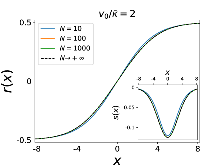
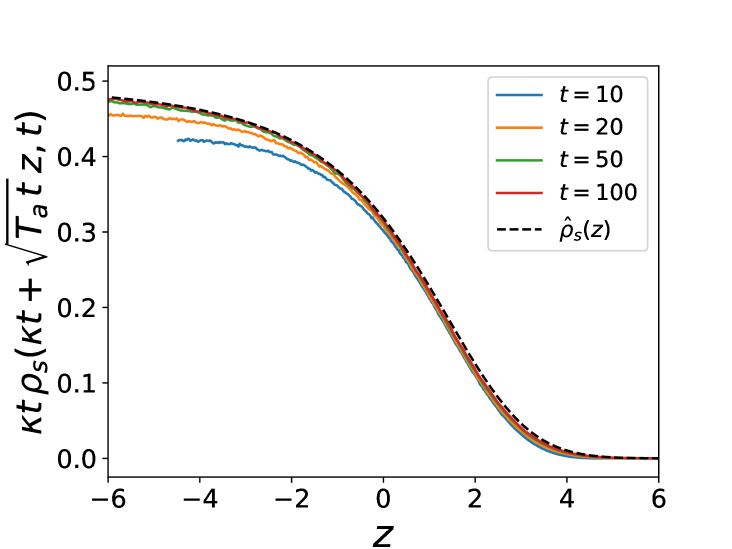
where we used again the condition $\bar{x}=0$ to fix the integration constant footnoteparity . One can check that for $v_{0}>\bar{\kappa}$, the function $f(r)$ is indeed invertible, see Fig. 3. The total density $\rho_{s}(x)=r^{\prime}(x)$ is even in $x$, while $\rho_{d}(x)=s^{\prime}(x)$ is odd in $x$, and both decay for $|x|\to+\infty$ as

Upon decreasing $\frac{v_{0}}{\bar{\kappa}}$ one sees from (18) that a transition must occur at $\frac{v_{0}}{\bar{\kappa}}=1$. Indeed at this point $f(r)=2r$, hence for $\frac{v_{0}}{\bar{\kappa}}=1$ the above solution (17) becomes

and $r(x)=\frac{1}{2}{\rm sgn}(x)$ and $s(x)=0$ for $|x|\geq x_{e}$. Hence the densities are non-zero in a finite interval $[-x_{e},x_{e}]$, with

and vanish for $|x|>x_{e}^{*}$, with step discontinuities at the two edges.

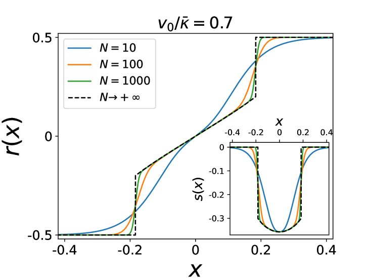
For $v_{0}<\bar{\kappa}$, $f(r)$ becomes non-invertible, as can be seen from Fig. 3. In this case the density has a finite support with edges at $\pm x_{e}$. More precisely, $f(r)$ is increasing only on an interval $[-r^{*},r^{*}]$ with $r^{*}=\frac{v_{0}}{2\bar{\kappa}}<\frac{1}{2}$. Since $r(x)$ should be increasing, one necessarily has $x_{e}\leq x^{*}=\frac{\bar{\kappa}}{\gamma}f(r^{*})$ and $r(x)$ must have shocks at $\pm x_{e}$. Since the r.h.s. in (16) is bounded, $r^{\prime}(x)$ can only diverge at a point where the prefactor in the l.h.s of (16) vanishes. Naively, this would lead to $r(x_{e})=r^{*}$, i.e. $x_{e}=x^{*}$. However, at the position of a shock, the interaction term should be interpreted with care, as for the standard Burgers equation. Due to the convention ${\rm sgn}(0)=0$, the force exerted on a cluster of particles at position $x_{e}$ is $\bar{\kappa}(\frac{1}{2}-r(x_{e}^{+}))-\bar{\kappa}(r(x_{e}^{-})+\frac{1}{2})=-\bar{\kappa}(r(x_{e}^{+})+r(x_{e}^{-}))$. Integrating equations (13-14) from $x_{e}^{-}$ to $x_{e}^{+}$ then gives SM

with $\Delta r=r(x_{e}^{+})-r(x_{e}^{-})$ and similarly for $\Delta s$. A non-zero $\Delta r$ then implies $r(x_{e}^{+})+r(x_{e}^{-})=v_{0}/\bar{\kappa}$ leading to

since $r(x_{e}^{+})=1/2$. For $|x|<x_{e}$, the prefactor in the l.h.s of (16) is strictly positive, and thus $r(x)$ is still given by (17), while for $|x|>x_{e}$ one has $r(x)=\frac{1}{2}$. This means that $\rho_{s}(x)$ has delta peaks at $\pm x_{e}$ each containing a fraction $1-\frac{v_{0}}{\bar{\kappa}}$ of particles. $s(x)$ is still given by (15) and thus it also has jumps of amplitude $1-\frac{v_{0}}{\bar{\kappa}}$ at $\pm x_{e}$. This implies that all the particles inside the cluster at $\pm x_{e}$ have $\sigma=\pm 1$ respectively. Note that as $\frac{v_{0}}{\kappa}\to\frac{1}{2}$, $x_{e}\to 0$ leading to a unique delta peak in $\rho_{s}(x)$ at $x=0$, consistent with the stability argument given above.

The existence of these edge clusters can be understood as follows. If there were no clusters, the rightmost particle would be subject to a force $\bar{\kappa}(1-\frac{1}{N})$ towards the left. Thus when $\bar{\kappa}>v_{0}$, for large enough $N$ it will always move towards the left even if it has an intrinsic velocity $+v_{0}$. It will then aggregate with other $+$ particles, until the resulting cluster reaches a fraction $n_{c}/N:=\frac{1}{2}-r(x_{e}^{-})$ of the total number of particles large enough to be at dynamical equilibrium, i.e. $v_{0}=\bar{\kappa}(1-n_{c}/N)$, from which we recover (21). For finite $N$ however, the size of this cluster will fluctuate, hence its position as well, and therefore we will observe a finite peak in the density instead of a delta function.

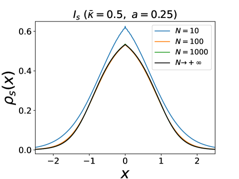
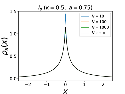
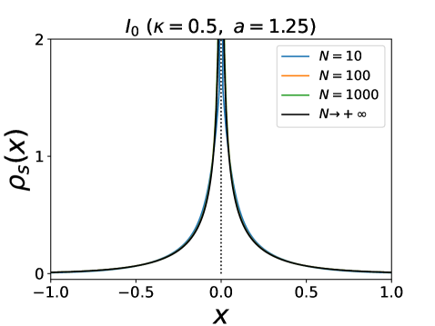
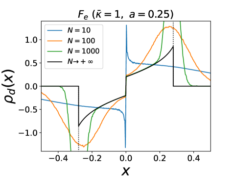
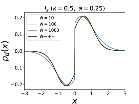
These predictions for $r(x)$ and $s(x)$ are compared with numerical simulations in Fig. 4. For $v_{0}>\bar{\kappa}$, the agreement is good even at very small values of $N$ ($N\sim 10$). For $\frac{\bar{\kappa}}{2}<v_{0}<\bar{\kappa}$, a distinct phase is predicted for $N=+\infty$. The numerics for finite $N$ clearly shows precursor signatures of this phase: as one can see on Fig. 3 a bimodal form of the density is already visible for small values of $N>2$. Furthermore the agreement on Fig. 4 at large $N$ for $r(x)$ and $s(x)$ is also very good. The behavior near the edges and analytical expression for the moments of the particle positions are obtained in SM .

Repulsive case. We now consider the repulsive case $\kappa=-\bar{\kappa}>0$, still for $V(x)=0$,

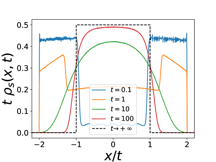
Since there is no confining potential to balance the repulsion between particles, all the particles escape at infinity and there is no stationary state. As in the case of passive particles, studied in PLDRankedDiffusion ; FlackRD , one expects that the size of the cloud grows linearly with time. Hence we will look for a large time solution of (22-23), as a scaling function of $y=x/t$ in the form

At leading order 0 one has

The solution is either $r_{0}^{\prime}(y)=0$ or $r_{0}(y)=y/(2k)$ i.e. one has

which leads to an expanding plateau

where $\theta(x)$ is the Heaviside distribution. Hence the scaled density $\rho_{s}$ takes the form of an expanding plateau, exactly as for passive particles PLDRankedDiffusion ; FlackRD . This is not too surprising since at large time the particles are far from each other hence the active noise averages out to diffusive noise. There are however non trivial fluctuations with slow decay at large time. Indeed, the second equation gives

hence one finds

Thus $\rho_{d}=0$ inside the plateau, i.e. $\rho_{+}=\rho_{-}$ (to leading order in $1/t$) but there is an excess of $-$ particles on the left edge and $+$ on the right edge with total weight decaying as $1/t$.

It is important to note that the $1/t$ expansion (24) is valid inside the plateau footnoter1 but fails at the edges. A more careful analysis in a region of width $\sim\sqrt{t}$ near the edges shows SM that the solution takes a boundary layer form (at the right edge)

with $T_{\rm eff}=T+T_{a}=T+\frac{v_{0}^{2}}{2\gamma}$. The boundary layer scaling function $\hat{\rho}_{s}(y)$ is identical to the one obtained for the passive problem FlackRD . This shows that for the expanding repulsive gas the role of the active noise is not different from that of passive noise at temperature $T_{a}=\frac{v_{0}^{2}}{2\gamma}$. Accordingly, note that the relation $\rho_{d}\simeq-\frac{v_{0}}{2\gamma}\partial_{x}\rho_{s}$ holds at large time both in the boundary layer and in the plateau (which we have checked numerically). These results show that the delta function in (30) has a finite width at finite time, i.e contrary to the attractive case there are no clusters. In fact the $\pm$ population imbalance $\sim 1/t$ is subdominant compared to the total population in the boundary layer $\sim 1/\sqrt{t}$.

We have checked these predictions numerically. Figure 5 shows the convergence of the density $\rho_{s}$ to (27) as time increases. The signature of the active noise is visible at short times: for $t<1/\gamma$, the particles split into two packets with a spread in velocities $\frac{x}{t}\in[v_{0},v_{0}+\kappa]$ (and same with minus), leading to two distinct blocks in the density, which disappear at larger time as the active noise averages out. One also sees in Figure 5 peaks forming the scaled $t^{2}\rho_{d}(x,t)$ as well as a numerical check of the boundary layer forms (Non-equilibrium phase transitions in active rank diffusions).

Linear potential. We now consider the case where the particles are submitted to an attractive linear potential $V(x)=a|x|$, $a>0$. For non-interacting particles $\bar{\kappa}=0$ there is a steady state with two phases, either $a<v_{0}$ and

or $a>v_{0}$ and $\rho_{s}(x)=\delta(x)$ DKM19 .

In presence of interactions, the large time behavior for large $N$ is richer and represented on the phase diagram in Fig. 6. There are six distinct phases which we briefly describe, four of them being stationary, while the other two are expanding (see SM for details and some plots of the densities).

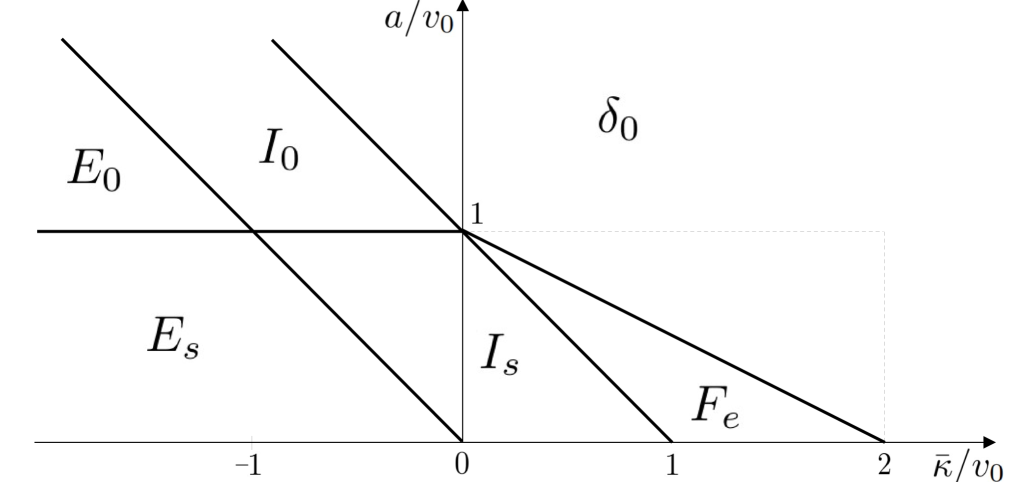
$\delta_{0}$ phase. It exists both in the attractive case, for $a>v_{0}-\frac{\bar{\kappa}}{2}$, and in the repulsive case, $a>v_{0}+\kappa$. The density is formed of a single cluster at $x=0$, $\rho_{s}(x)=\delta(x)$. Note that outside the dotted lines in Fig. 6 it already exists for finite $N$, while inside the density has a finite width for finite $N$.

$I_{s}$ phase, both in the attractive case, for $a<v_{0}-\bar{\kappa}$, and in the repulsive case, for $\kappa<a<v_{0}$. This phase is quite similar to the one for $a=0$. The function $r=r(x)$ is odd and is given for $x\geq 0$ as the solution of

an extension of (17) above. From $r(x)$ one obtains for any $x\in\mathbb{R}$

The densities are given in parametric form for $x\geq 0$ and $r\in[0,1/2]$ as

They have infinite support and are smooth except at $x=0$ where $\rho_{d}(x)$ has a jump and $\rho_{s}(x)$ has a linear cusp.

$F_{e}$ phase, in the attractive case, for $v_{0}-\bar{\kappa}<a<v_{0}-\frac{\bar{\kappa}}{2}$. Here ${\sf f}_{a}(r)$ becomes non-invertible. The densities have a finite support $[-x_{e},x_{e}]$ with shocks at the two edges $\pm x_{e}$ such that

with $\gamma x_{e}={\sf f}_{a}(r(x_{e}^{-}))$. It corresponds to clusters with a fraction $\frac{\bar{\kappa}+a-v_{0}}{\bar{\kappa}}$ of the particles (all being $+$ at $x=x_{e}$ and $-$ at $x=-x_{e}$). Inside the support, $r(x)$ is again given by (33), $s(x)$ by (34) and the densities by (35), with the same singular behavior at $x=0$.

$I_{0}$ phase, in the repulsive case, for $\kappa<a<v_{0}+\kappa$ and $a>v_{0}$. This phase is similar to $I_{s}$ but has a shock at $x=0$ corresponding to a cluster with equal fractions of $\pm$ particles and of total weight $\frac{a-v_{0}}{\kappa}$. The function $r(x)$ for $x>0$ is now given by

From (37), (33) and (34) (which still holds for $x\neq 0$) we obtain that $\rho_{s}(x)$ and $\rho_{d}(x)$ exhibit near $x=0$ an inverse square root divergence

with $B=\frac{1}{2\kappa}\sqrt{\frac{\gamma}{v_{0}}(v_{0}^{2}-(a-\kappa)^{2})}$, which involves only $+$ particles for $x>0$ and $-$ particles for $x<0$.

$E_{s}$ and $E_{0}$ phases, in the repulsive case, for $a<\kappa$ and $a<v_{0}$ or $a>v_{0}$ respectively. In this case a fraction $1-\frac{a}{\kappa}$ of particles escape to infinity, while a fraction $\frac{a}{\kappa}$ remain confined. Under the scaling $|x|\sim t$ one finds at large time in both phases

hence the expanding part behaves similarly as for $a=0$, i.e. it is uniform within the support, which now spreads with velocities $\pm(\kappa-a)$. Similarly one finds

Both densities are smooth on scales $\sqrt{t}$, with similar boundary layers near the edges as for $a=0$ (see above and SM ).

For the particles which remain bound within $x=O(1)$, $r(x)$ is smooth away from $x=0$ given by, for $x>0$

where in the phase $E_{0}$, i.e. $a>v_{0}$, there is a cluster at $x=0$ containing a fraction $\frac{a-v_{0}}{\kappa}$ of the total number of particles. From (41) one obtains an explicit formula for the densities, see SM . The most notable feature is that they decay as power laws at large distance, in both phases

while in the phases $I_{s}$ and $I_{0}$ the densities decay exponentially at large distance. In that sense in the phases $E_{s}$ and $E_{0}$ the steady state of the bound particles is always critical. Indeed, the bound particles can be effectively described by an interaction constant $\kappa_{\rm eff}=a$, see SM . Finally, the non-analytic behavior of the densities near $x=0$ is similar to the one in the phases $I_{s}$ and $I_{0}$. In SM we compare these results with the case of passive particles, where only the phases $I_{s}$ and $E_{s}$ are present.

More general interactions. Consider now a pairwise interaction potential $W(x)$, such that the force term in (1) is replaced by $-\frac{1}{N}\sum_{j}W^{\prime}(x_{i}-x_{j})$, Eq. (1) being recovered for $W(x)=\bar{\kappa}|x|$. $W^{\prime}(x)$ being odd, we restrict to the case $W^{\prime}(0)=0$, i.e. we exclude the possibility that $W^{\prime}(x)$ diverges at $x=0$ for which the large $N$ limit is problematic TouzoDBM2023 . At large $N$, from (Non-equilibrium phase transitions in active rank diffusions) with the replacement $\bar{\kappa}\,{\rm sgn}(x-y)\to W^{\prime}(x-y)$ we obtain at stationarity

where

Eqs. (43) are identical to those of a single RTP in an effective force field $\tilde{F}(x)$ which itself depends on the density. They can be solved formally, leading (in the simplest case, see SM ) to

where $K$ is determined by the normalization. Eqs. (44) and (45) are self-consistent equations for the density $\rho_{s}(x)$. In SM we show how it recovers the above results for the rank interaction. For a harmonic interaction the density at large $N$ is found to be the same as for a single particle in a harmonic well. Other examples will be studied in inprep .

Conclusion. We have obtained a description of an active version of rank diffusion, controlled at large $N$. We have computed exactly the densities of RTP particles at large time in that limit. In particular, in the attractive case we found a collective dynamical phase transition in the steady state where the support of the density changes from infinite to finite, with shocks (i.e clusters of particles) appearing at the edges. In presence of a linear confining potential we find a rich phase diagram with six phases. In the expanding phases we find that a fraction of the particles remain bound, and in a critical state with power-law decay of the densities at large distance. We also obtained a self-consistent equation for the densities which opens the way to treat more general interaction potentials. Some remaining open questions are finite $N$ fluctuations and calculation of other observables, such as entropy production.

Acknowledgments: We thank Gregory Schehr for collaborations on related topics. We thank LPTMS (Orsay) and Collège de France for hospitality.

.

.

We give the principal details of the calculations described in the main text of the Letter. We display additional analytical and numerical results which support the findings presented in the Letter.

References

- (1) J. Masoliver and K. Lindenberg, Continuous time persistent random walk: a review and some generalizations, Eur. Phys. J. B 90, 1 (2017).
- (2) M. Kac, A stochastic model related to the telegrapher’s equation, Rocky Mountain J. Math. 4, 497 (1974).
- (3) H. C. Berg, E. Coli in Motion, (Springer Verlag, Heidel- berg, Germany) (2004).
- (4) J. Tailleur, and M. E. Cates, Statistical mechanics of interacting run-and-tumble bacteria, Phys. Rev. Lett. 100, 218103 (2008).
- (5) M. C. Marchetti, J. F. Joanny, S. Ramaswamy, T. B. Liverpool, J. Prost, M. Rao, and R. Aditi Simha, Hydrodynamics of soft active matter, Rev. Mod. Phys. 85, 1143 (2013).
- (6) A. B. Slowman, M. R. Evans, and R. A. Blythe, Jamming and attraction of interacting run-and-tumble random walkers, Phys. Rev. Lett. 116, 218101 (2016).
- (7) A. B. Slowman, M. R. Evans, and R. A. Blythe, Exact solution of two interacting run-and-tumble random walkers with finite tumble duration, J. Phys. A: Math. Theor. 50, 375601 (2017).
- (8) Y. Fily, and M. C. Marchetti, Athermal phase separation of self-propelled particles with no alignment, Phys. Rev. Lett. 108, 235702 (2012).
- (9) M. Cates, and J. Tailleur, Motility-induced phase separation, Annu. Rev. Condens. Matter Phys. 6, 219 (2015).
- (10) C. M. Barriuso Gutiérrez, C. Vanhille-Campos, Francisco Alarcon, I. Pagonabarraga, R. Britoai, and C. Valeriani, Collective motion of run-and-tumble repulsive and attractive particles in one-dimensional systems, Soft Matter 17(46) (2021).
- (11) R. Soto, R. Golestanian, Run-and-tumble dynamics in a crowded environment: Persistent exclusion process for swimmers, Phys. Review E 89, 012706 (2014).
- (12) P. Le Doussal, S. N. Majumdar, G. Schehr, Stationary nonequilibrium bound state of a pair of run and tumble particles, Physical Review E 104(4), 044103 (2021).
- (13) P. Dolai, S. Krekels, and C. Maes, Inducing a bound state between active particles, Phys. Rev. E 105, 044605 (2022).
- (14) I. Mukherjee, A. Raghu, and P. K. Mohanty, Nonexistence of motility induced phase separation transition in one dimension, SciPost Phys. 14, 165 (2023) .
- (15) E. Mallmin, R. A. Blythe, and M. R. Evans, Exact spectral solution of two interacting run-and-tumble particles on a ring lattice, J. Stat. Mech., 013204 (2019).
- (16) A. Das, A. Dhar, and A. Kundu, Gap statistics of two interacting run and tumble particles in one dimension, J. Phys. A: Math. Theor. 53, 345003 (2020).
- (17) P. Le Doussal, S. N. Majumdar, and G. Schehr, Noncrossing run-and-tumble particles on a line, Phys. Rev. E 100, 012113 (2019).
- (18) P. Singh, A. Kundu, Crossover behaviours exhibited by fluctuations and correlations in a chain of active particles, J. Phys. A: Math. Theor. 54, 305001 (2021)
- (19) S. Put, J. Berx, and C. Vanderzande, Non-Gaussian anomalous dynamics in systems of interacting run-and-tumble particles, J. Stat. Mech. 123205 (2019).
- (20) M. J. Metson, M. R. Evans, and R. A. Blythe, Tuning attraction and repulsion between active particles through persistence, EPL 141, 41001 (2023).
- (21) M. J. Metson, M. R. Evans, and R. A. Blythe, From a microscopic solution to a continuum description of interacting active particles, Phys. Rev. E 107, 044134 (2023).
- (22) R. Dandekar, S. Chakraborti, and R. Rajesh, Hard core run and tumble particles on a one-dimensional lattice, Phys. Rev. E 102, 062111 (2020).
- (23) A. G. Thompson, J. Tailleur, M. E. Cates, R. A. Blythe, Lattice models of nonequilibrium bacterial dynamics, J. Stat. Mech. P02029 (2011).
- (24) L. Touzo, P. Le Doussal, G. Schehr, Interacting, running and tumbling: the active Dyson Brownian motion, EPL 142, 61004 (2023) and arXiv:2302.02937.
- (25) A. D. Banner, R. Fernholz, I. Karatzas, Atlas models of equity markets, Ann. Appl. Probab. 15, 2296 (2005)
- (26) S. Pal, J. Pitman, One-dimensional Brownian particle systems with rank-dependent drifts, Ann. Appl. Probab. 18, 2179 (2008).
- (27) G. B. Rybicki, Exact statistical mechanics of a one-dimensional self-gravitating system, Astrophys. Space Sci. 14, 56 (1971).
- (28) P. H. Chavanis, C. Sire, Anomalous diffusion and collapse of self-gravitating Langevin particles in dimensions, Phys. Rev. E 69, 016116 (2004).
- (29) A. Lenard, Exact statistical mechanics of a one-dimensional system with Coulomb forces, J. Math. Phys. 2, 682 (1961).
- (30) R. J. Baxter, Statistical mechanics of a one-dimensional Coulomb system with a uniform charge background, Proc. Camb. Phil. Soc. 59, 779 (1963)
- (31) G. Tellez, E. Trizac, Screening like charges in one-dimensional Coulomb systems: Exact results, Phys. Rev. E 92, 042134 (2015).
- (32) For a recent review, see M. Lewin, Coulomb and Riesz gases: The known and the unknown, J. Math. Phys. 63, 061101 (2022).
- (33) A. Dhar, A. Kundu, S. N. Majumdar, S. Sabhapandit, G. Schehr, Exact extremal statistics in the classical 1d Coulomb gas, Phys. Rev. Lett. 119, 060601 (2017).
- (34) A. Flack, S. N. Majumdar, G. Schehr, Gap probability and full counting statistics in the one-dimensional one-component plasma, J. Stat. Mech. 053211 (2022).
- (35) D. Chafai, D. Garcia-Zelada, P. Jung, At the edge of a one-dimensional jellium, Bernoulli 28, 1784 (2022).
- (36) P. Le Doussal, Ranked diffusion, delta Bose gas and Burgers equation, Phys. Rev. E 105, L012103 (2022).
- (37) D. S. Dean, Langevin Equation for the density of a system of interacting Langevin processes, J. Phys. A: Math. Gen. 29, L613 (1996).
- (38) K. Kawasaki, Microscopic analyses of the dynamical density functional equation of dense fluids, J. Stat. Phys. 93, 527 (1998).
- (39) A. Flack, P. Le Doussal, S. N. Majumdar, G. Schehr, Out of equilibrium dynamics of repulsive ranked diffusions: the expanding crystal, Phys. Rev. E 107, 064105 (2023).
- (40) P. Le Doussal and G. Schehr, unpublished.
- (41) See supplementary material
- (42) Since f(r) is odd, this is the same as imposing .
- (43) Note however that the higher order terms, e.g. , depend on the initial condition SM .
- (44) A. Dhar, A. Kundu, S. N. Majumdar, S. Sabhapandit and G. Schehr, Run-and-tumble particle in one-dimensional confining potentials: Steady-state, relaxation, and first-passage properties, Phys. Rev. E 99, 032132 (2019).
- (45) Solutions with , with a shock at are in principle possible but are excluded by our numerical results.
- (46) L. Touzo, P. Le Doussal to be published.
.
Supplementary Material for
Active rank diffusion