Non-Hermitian invisibility in tight-binding lattices

Let us consider wave scattering from a time-dependent NH potential or defect on a one-dimensional single-band tight-binding lattice, which in physical space is described by the coupled equations for the wave amplitudes $\psi_{n}(t)$ at various lattice sites $n$

where $\kappa_{l}=\kappa_{-l}^{*}$ is the hopping amplitude between lattice sites distant $|l|$ on the lattice and the perturbation matrix $V_{n.l}(t)$ describes the time-dependent scattering potential or lattice defects, which is assumed to vanish fast enough as $|n,l|\rightarrow\infty$. For example, for a local on-site scattering potential the matrix $V_{n,l}(t)$ is diagonal, while for defects of the hopping amplitudes the matrix $V_{n,l}(t)$ contains off-diagonal non-vanishing elements. As for the time dependence of the perturbation matrix, special cases are those of a stationary (i.e. time-independent) or time-periodic potentials. However, we assume here a rather general dependence of time with the only constraint that $|V_{n,l}(t)|$ is a bounded function of time, i.e. it does not secularly grow in time, and can be expanded as a Fourier integral or generalized Fourier integral (i.e. containing undamped harmonic terms).

In the absence of the scattering potential, $V_{n,l}(t)=0$, the eigenstates of Eq.(1) are extended Bloch waves, $\psi_{n}(t)=\exp[iqn-iE(q)t]$, with energy $E=E(q)$ defined by the dispersion relation

A wave packet with carrier Bloch wave number $q$ propagates on the lattice with a group velocity $v_{g}=(dE/dq)$. For a lattice with short-range hopping, i.e. when $|\kappa_{l}|\rightarrow 0$ fast enough as $|l|\rightarrow\infty$, the group velocity displays un upper bound, according to Lieb and Robinson Lieb . Likewise, the energy band displays a finite width $\Delta$. For example, for a tight-binding lattice with nearest-neighbor hopping amplitude, $\kappa_{l}=0$ for $l\neq\pm 1$ and $\kappa_{l}=\kappa$ for $l=\pm 1$, the tight-binding dispersion curve reads $E(q)=-2\kappa\cos q$, the energy band has a finite width given by $\Delta=4\kappa$, and the group velocity $v_{g}=2\kappa\sin q$ displays the upper bound $v_{m}=2\kappa=\Delta/2$.

Let us now consider a spatially-localized time-dependent scattering potential and/or lattice defects, described by the time-dependent perturbation matrix $V_{n,m}(t)$ with $V_{n,m}(t)\rightarrow 0$ fast enough as $|n,m|\rightarrow\infty$. In particular, for a local on-site scattering potential $V_{n}(t)$ the perturbation matrix $V_{n,m}(t)$ is diagonal and given by $V_{n,m}(t)=V_{n}(t)\delta_{n,m}$. We assume that a Bloch (plane) wave with wave number $q$, energy $E=E(q)$ and positive group velocity $v_{g}>0$, coming from $n=-\infty$, is incident from the left side toward the scattering region. We can write the solution to Eq.(1) in the form

where the former term on the right hand side of Eq.(3) is the incoming plane wave while $\phi_{n}(t)$ are the amplitudes of scattered wave on the lattice, which satisfy the coupled equations

Equation (4) is a linear non-autonomous system with a forcing term in the variables $\phi_{n}(t)$ and should be solved with the appropriate boundary conditions, which depend rather generally on the time-dependence of the scattering perturbation matrix $V_{n,m}(t)$. For a static (time-independent) potential, the system is autonomous, $\phi_{n}(t)$ is independent of $t$ and outgoing boundary conditions should be imposed. The same holds for a time-periodic potential, where Floquet analysis can be used r16c . On the other hand, for arbitrary time-dependence of the potential Eq.(4) should be solved by considering the initial-value condition $\phi_{n}(-t_{0})=0$ at some remote time $t_{0}\rightarrow\infty$. Here we will consider this rather general case. In this case the NH scattering matrix $V_{n,m}(t)$ turns out to be invisible provided that, for any arbitrary incident wave, one has $\phi_{n}(t)\rightarrow 0$ for the scattered wave amplitudes as $|n|\rightarrow\infty$ for any time instant $t$.

In the limit of a tight-binding lattice with nearest-neighbor hopping of amplitude $\kappa$ and for an on-site scattering potential $V_{n}(t)$, i.e. $V_{n,m}(t)=V_{n}(t)\delta_{n,m}$, we can solve Eq.(1) by letting $\psi_{n}(n)=\psi(x=n,t)$, where the wave function $\psi(x,t)$ of continuous space and time variables $x$ and $t$ satisfies the discrete Schrödinger equation (see for instance K1 ; r41 )

where $p_{x}=-i\partial_{x}$ and $V_{n}(t)=V(x=n,t)$.
The kinetic energy term in Eq.(5) is periodic in the momentum $p_{x}$, which implies that a limited interval of energies are allowed in a lattice system, corresponding to propagative (Bloch) waves. The invisibility method that will be presented in the next section works provided that the kinetic energy operator is bounded, like in a system with discrete translational invariance, but breaks down when the kinetic energy term is unbounded from above, like in a system with continuous translational symmetry. This case is found in the so-called long-wavelength limit of the discrete Schrödinger equation, which corresponds to low-energy excitation of the system. Specifically, for a potential $V(x,t)$ that varies slowly with respect to $x$ over the lattice period and for low-energy excitation of the system, we may expand the kinetic energy operator $\cos(p_{x})$ in the neighbor of $p_{x}=0$, i.e. we may let $\cos(p_{x})\simeq 1-p_{x}^{2}/2$ (long-wavelength approximation). In this case, omitting an inessential constant energy potential term, Eq.(5) reads

which is the continuous Schrödinger equation describing the scattering of a quantum particle in the NH time-dependent potential $V(x,t)$. In this limit we loose the discrete translational invariance of the lattice and the energy of the system becomes unbounded from above.

NH invisibility in lattice systems has been predicted in some previous works, including nearest-neighbor tight-binding lattices under special stationary potentials synthesized by the methods of supersymmetry r9a or for harmonically-oscillating on-site potentials r16c , and for the class of Kramers-Kronig potentials drifting on the lattice at a speed faster than $v_{g}$ K2 . The last method exploits the finite speed of wave propagation in the lattice, so that any potential that drifts on the lattice at a speed faster than $v_{m}$ cannot reflect waves and thus is transparent.

Here we widen the class of NH invisible potentials on a lattice, beyond the nearest-neighbor approximation and including also scattering from off-diagonal (hopping) defects in addition to on-site (diagonal) potential, exploiting the finiteness of the energy bandwidth of the lattice. The main physical idea is as follows. Let us assume that the Fourier spectrum $\hat{V}_{n,m}(\omega)$ of the perturbation scattering matrix $V_{n,m}(t)$, defined by

vanishes for all frequencies $\omega<\omega_{0}$ (or, likewise, for any frequency $\omega>-\omega_{0}$), where $\omega_{0}$ is larger than the bandwidth $\Delta$ of the tight-binding lattice. The interaction of the incidente wave with the time-varying potential is inelastic and involves the absorption or emission of energy quanta from the oscillating potential uffa1 ; uffa2 . However, since the Fourier spectrum of the oscillating potential is composed by $\omega>\omega_{0}$ frequency components solely, the energies $E^{{}^{\prime}}$ of the scattered wave are constrained by the inequality r16c ; uffa3 $E^{{}^{\prime}}=E+\omega>E+\omega_{0}>E+\Delta$, i.e. they fall outside the allowed energy band of the lattice. Therefore, far from the scattering region where the lattice is uniform, the scattered waves are Bloch waves but with an imaginary Bloch wave number, i.e. they are evanescent waves decaying toward zero as $|n|\rightarrow\infty$. This means that the scattered waves cannot be propagative in the homogeneous lattice regions, far from the scattering potential, which clearly implies invisibility.
We emphasize that this result holds regardless of the specific spatial shape of the potential and specific shape of incoming waves, so that the kind of invisibility induced by the temporal modulation does not require any special tailoring in space of the scattering potential nor special initial excitation of the system with prescribed input state (such as e.g. in Ref.A6 ). From this simple physical picture, we can conclude that the following general property holds:
Any scattering NH matrix perturbation $V_{n,m}(t)$ such that its Fourier spectrum vanishes for frequencies $\omega<\omega_{0}$ (or likewise for frequencies with $\omega>-\omega_{0}$), with $\omega_{0}$ larger than the width $\Delta$ of the tight-binding lattice band, is invisible
To prove the above general property, let us integrate the coupled equations (4) for the scattered wave amplitudes $\phi_{n}(t)$ at various lattice sites with the initial condition $\phi_{n}(-t_{0})=0$ at a far remote time $t_{0}\rightarrow\infty$ using a modified Laplace-Fourier method. To this aim, let $f(t)$ be a regular function of time $t$, defined for $t\geq-t_{0}$ and bounded (or growing in time lower than any exponential) as $t\rightarrow\infty$. For a given time $t_{1}>0$, arbitrarily large, let us introduce the modified Fourier-Laplace spectrum

where $\epsilon>0$ is a small positive number. Note that the previous relation reduces to the usual Fourier spectrum in the limit $\epsilon=0$ and $t_{1},t_{0}\rightarrow\infty$. The inverse relation to Eq.(8) reads (see Appendix)

which is valid for $-t_{0}<t<-t_{1}$.
Here we are interested in considering the triple limit $t_{0},t_{1}\rightarrow\infty$, $\epsilon\rightarrow 0^{+}$ with $\epsilon t_{0}\rightarrow 0$ and $\epsilon t_{1}\rightarrow\infty$. Multiplying both sides of Eq.(4) by $\exp(i\omega t-\epsilon t)$ and integrating over time $t$ from $-t_{0}$ to $t_{1}$, taking into account that $\phi_{n}(-t_{0})\exp(\epsilon t_{0})\simeq\phi_{n}(-t_{0})=0$ and $\phi_{n}(t_{1})\exp(-\epsilon t_{1})\simeq 0$ in the above mentioned limit, one obtains

In deriving Eq.(10), we used the relation

which is valid in the large $t_{0},t_{1}$ limit, as shown in the Appendix. Since $\hat{V}_{n,l}(\Omega)=0$ for $\Omega<\omega_{0}$, from Eq.(10) it readily follows that the spectral amplitude $\hat{\phi}_{n}^{(\epsilon)}(\omega)$ depends on all other spectral amplitudes $\hat{\phi}_{l}^{(\epsilon)}(\omega^{\prime})$ at frequencies $\omega^{\prime}<\omega-\omega_{0}$. Moreover, in the large $t_{0},t_{1}$ and small $\epsilon$ limits, $\hat{V}_{n,l}^{(\epsilon)}(\omega)\simeq\hat{V}_{n,l}(\omega)=0$ for $\omega>\omega_{0}$ (see Appendix), so that the forcing term of the spectral amplitude $\hat{\phi}_{n}^{(\epsilon)}(\omega)$ [the term on the right hand side of Eq.(10)] vanishes for $\omega<\omega_{0}$. This implies that

for any frequency $\omega\leq\omega_{0}$, in agreement with the physical picture that the scattered waves cannot transport energies (frequencies) smaller than $E+\omega_{0}$. Therefore we can write

Let us now consider the behavior of $\phi_{n}(t)$ as $n\rightarrow\pm\infty$, i.e. far from the scattering region. In this limit, the spectral amplitudes $\hat{\phi}_{n}^{(\epsilon)}(\omega)$ with $\omega>\omega_{0}$ satisfy the linear dispersion equation

which is obtained from Eq.(10) by neglecting the vanishing scattering matrix elements as $n\rightarrow\pm\infty$. The solution to Eq.(14) is given in terms of superposition of Bloch waves, namely $\hat{\phi}_{n}^{(\epsilon)}(\omega)\sim Y_{\pm}(\omega)\exp(iQ_{\pm}n)$ as $n\rightarrow\pm\infty$ with some complex amplitudes $Y_{\pm}(\omega)$ and complex Bloch wave numbers $Q_{\pm}=Q_{\pm}(\omega)$. The complex Bloch wave numbers are obtained as a solution of the dispersion equation

with ${\rm Im}(Q_{+})<0$ and ${\rm Im}(Q_{-})>0$ Since the energy $E+\omega>E+\Delta$ falls outside the band, the imaginary parts of $Q_{\pm}$ are strictly nonvanishing and thus the Bloch waves $\hat{\phi}_{n}^{(\epsilon)}(\omega)$ are evanescent, exponentially decaying as $n\rightarrow\pm\infty$ for any frequency $\omega>\omega_{0}$. Indicating by $Q_{+,m}>0$ the minimum of $|{\rm Im}(Q_{+})|$ over the range of frequencies $\omega\geq\omega_{0}$, from Eq.(13) for $n\rightarrow\infty$ one has

and thus $|\phi_{n}(t)|\rightarrow 0$ as $n\rightarrow\infty$ for any time instant $t$. Likewise, one has $|\phi_{n}(t)|\rightarrow 0$ as $n\rightarrow-\infty$ for any time instant $t$, indicating that the NH scattering perturbation matrix is invisible.

Clearly, the invisibility property strictly requires a finite bandwidth of allowed energies in the system, and thus it breaks down in the continuous (long-wavelength) limit of lattice dynamics. In fact, in this limit the dynamics can be described by a usual continuous Schrödinger equation [Eq.(6)] with an unbounded range of allowed energies. Since the energies $E^{\prime}$ of scattered waves can now fall into allowed energy intervals, they are now propagative (rather than evanescent) waves, and the invisibility property is thus lost: Only for some special tailored space-time potentials scattering can be prevented (see for instance r26bis ).

To exemplify the main result presented in the previous subsection and to check the correctness of the theoretical analysis, let us consider a scattering matrix which can be factorized as

with a time-independent matrix $T_{n,m}$ and a function of time $R(t)$. An invisible potential is obtained, for example, by assuming for $R(t)$ a superposition of positive-frequency harmonics, i.e. $R(t)=\sum_{\alpha}A_{\alpha}\exp(i\omega_{\alpha}t)$, with frequencies $\omega_{\alpha}>\Delta$. The frequencies $\omega_{\alpha}$ could be rather generally incommensurate, so as a standard Floquet analysis of inelastic scattering r16c ; uffa1 cannot be applied. Yet our general analysis discussed in previous subsection predicts invisibility of the scattering potential. As for the form of the matrix $T_{n,m}$, we consider two typical cases. The first one corresponds to a local on-site scattering potential, i.e. $T_{n,m}=V_{n}\delta_{n,m}$, while the second case corresponds to a defect in the hopping amplitudes of the lattice, for example we can assume $T_{n,m}=\delta_{n,0}\delta_{m,1}+\delta_{n,1}\delta_{m,0}$, which corresponds to modify the hopping amplitude between sites $n=0$ and $n=1$ of the lattice from $\kappa_{1}$ to $\kappa_{1}+R(t)$.

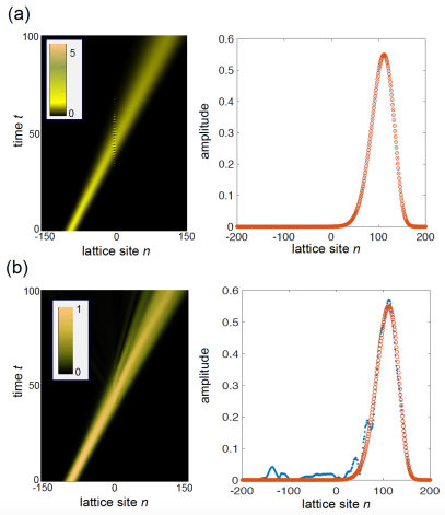
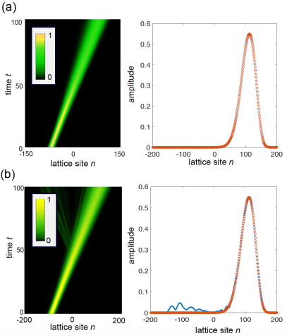
Figures 1 and 2 demonstrate the invisibility of the oscillating scattering perturbation in the two cases. The figures depict the evolution of a forward-propagating Gaussian wave packet, which is scattered off by the time-varying potential. At initial time $t=0$ the wave packet is localized at the left side far from the scattering region, and propagates forward toward the scattering region. Coupled equations (1) have been numerically solved using an accurate variable-step fourth-order Runge-Kutta method. We assumed a tight-binding lattice with nearest and next-to-nearest neighbor hopping amplitudes $\kappa_{1}=\kappa_{-1}=1$, $\kappa_{2}=\kappa_{-2}=0.2$ and $\kappa_{l}=0$ for $l\neq\pm 1,\pm 2$. The bandwidth of the lattice is $\Delta=4$. In Fig.1 we have a local scattering potential $V_{n}=V_{0}\exp(-n^{2}/w^{2})$ of amplitude $V_{0}=5$ and size $w=2$, while in Fig.2 we have a defect of the hopping amplitude between sites $n=0$ and $n=1$, described by the perturbation matrix $T_{n,m}=\delta_{n,0}\delta_{m,1}+\delta_{n,1}\delta_{m,0}$. Two different modulation functions $R(t)$ have been used, namely $R(t)=A_{1}\exp(i\omega_{1}t)+A_{2}\exp(i\omega_{2}t)$ [Figs.1(a) and 2(a)], and $R(t)=A_{1}\cos(\omega_{1}t)+A_{2}\cos(\omega_{2}t)$ [Figs.1(b) and 2(b)]. Parameter values are $A_{1}=A_{2}=1$, $\omega_{1}=5$, and $\omega_{2}=\sqrt{18}$. Note that in the former case the modulation function has a positive-frequency spectrum and, since $\omega_{1,2}>\Delta$, invisibility is clearly observed according to the theoretical analysis. Conversely, in the latter case the Fourier spectrum of $R(t)$ is bilateral, corresponding to an Hermitian perturbation, and invisibility is not anymore observed.

Synthetic lattices based on photonic, mechanical, acoustic, electrical or ultracold atomic systems could provide possible physical platforms for the observation of the invisibility effect predicted in this work. Here we discuss in details a possible experimental setup based on photonic quantum walks of light pulses in coupled fiber loops R28 . Photonic quantum walks realize a synthetic lattice in time domain, enabling a flexible control of non-Hermitian terms in the Hamiltonian. They have provided recently a fascinating platform to experimentally access a wealth of novel non-Hermitian phenomena, including parity-time symmetry breaking R29 ; R30 , non-Hermitian topological physics R31 ; R32 ; R33 ; R34 ; R34b , non-Hermitian Anderson localization R35 , constant-intensity waves and induced transparency in complex scattering potential A6 , and multiple non-Hermitian phase transitions R36 . The system consists of two fiber loops of slightly different lengths $L\pm\Delta L$ (short and long paths) that are connected by a fiber coupler with a coupling angle $\beta$. Two synchronized amplitude and phase modulators are placed in one of the two loops to control on demand the amplitude and phase of the traveling pulses at each transit. The traveling times of light in the two loops are $T\pm\Delta T$, where $T=L/c$, $c$ is the group velocity of light in the fiber at the probing wavelength, and $\Delta T=\Delta L/c\ll T$ is the time mismatch arising from fiber length unbalance. The light dynamics of the optical pulses at successive transits in the two loops is considered at discretized times $t=t_{n}^{m}=n\Delta T+mT$, where $n=0,\pm 1,\pm 2,...$ defines the site number of the synthetic lattice at various time slots and $m$ is the round-trip number, assumed to match the traveling time $T$ along the mean path length $L$. Indicating by $u_{n}^{(m)}$ and $v_{n}^{(m)}$ the field amplitudes at the discretized times $t_{n}^{m}$ of the pulses in the two loops, light dynamics in the coupled fiber loops is governed by the discrete-time coupled equations (see e.g. A6 ; K2b ; R30 ; R33 ; R34b ; R36 ; R37 )

where $V_{n}^{(m)}$ is the complex NH scattering potential that is realized by suitable control of synchronized phase and amplitude modulators. In the absence of the scattering potential, i.e. for $V_{n}^{(m)}=0$, the synthetic lattice shows discrete spatial invariance and the corresponding Bloch eigenfunctions to Eqs.(18) and (19) are given by $(u_{n}^{(m)},v_{n}^{(m)})^{T}=(\bar{u},\bar{v})\exp[iqn-iE(q)m]$, where $q$ is the spatial Bloch wave number and $E(q)$ is the quasi energy. Owing to the binary nature of the lattice, two quasi-energy bands are found with dispersion relations $E_{\pm}(q)$ given by

Note that for a coupling angle $\beta$ close to $\pi/2$, i.e. for $\beta=\pi/2-\rho$ with $|\rho|\ll 1$, the dispersion relations of the two quasi energies read

i.e. they correspond to the shifted dispersion curves of two tight-binding lattices with nearest-neighbor hopping amplitude $\kappa=\pm\rho/2$. In order to observe the NH invisibility predicted in this work, we consider the continuous-time limit of the discrete-time quantum walk R34b , which is obtained by assuming a coupling angle $\beta$ close to $\pi/2$, i.e. $\beta=\pi/2-\rho$ with $|\rho|\ll 1$, and a small and slowly-varying amplitude of the scattering potential amplitude, i.e. $|V_{n}^{(m)}|\sim O(\rho)\ll 1$ and $V_{n}^{(m+1)}\simeq V_{n}^{(m)}$. At first order in $\rho$, Eqs.(18) and (19) take the form

From the above equations, one can eliminate from the dynamics the variables $v_{n}^{(m)}$, yielding a second-order difference equation for $u_{n}^{(m)}$, which is solved by letting R34b

In Eq.(24), $\psi^{(\pm)}_{n}(m)$ are slowly-varying functions of the discrete time $m$ which satisfy the decoupled continuous-time Schrödinger equations

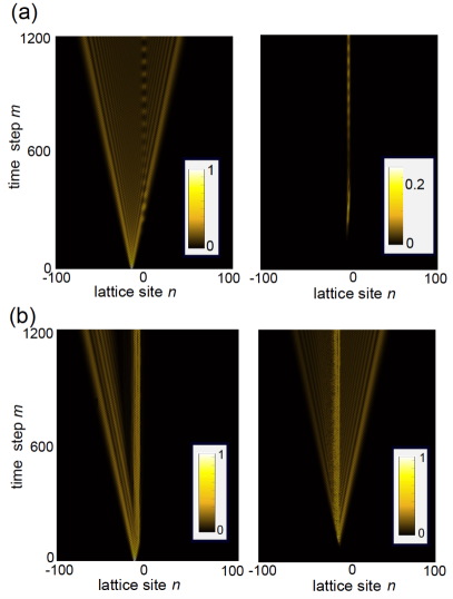
where we have set $\kappa\equiv(\rho/2)$, $t=m$ (considered as a continuous variable) and $V_{n}(t)=V_{n}^{(m)}$. Therefore, in the continuous-time limit the light pulse dynamics in the photonic quantum walk setup emulates the scattering dynamics from a NH time-dependent potential $V_{n}(t)$ on two independent tight-binding lattices with nearest-neighbor hooping amplitudes $\pm\kappa$. Provided that the Fourier spectrum of the potential $V_{n}(t)$ vanishes for all frequencies $\omega$ smaller than the bandwidth $4\kappa$ of the tight-binding lattices, the scattering potential turns out to be invisible. An illustrative example, showing an invisible potential in the quantum walk system, is shown in Fig.3. The figure depicts the numerically-computed light pulse dynamics in the coupled fiber loops, as obtained by solving the discrete-time coupled equations (18) and (19), i.e. without any approximation, for a coupling angle $\beta=0.97\times\pi/2$ and for a scattering potential $V_{n}^{(m)}=R_{m}\exp[-(n/3)^{2}]$ with modulation function $R_{m}=A_{1}\exp(i\omega_{1}m)+A_{2}\exp(i\omega_{2}m)$ in Fig.3(a), and $R_{m}=A_{1}\cos(\omega_{1}m)+A_{2}\cos(\omega_{2}m)$ in Fig.3(b) ($A_{1}=0.1$, $A_{2}=0.06$, $\omega_{1}=0.1$, $\omega_{2}=\sqrt{2}/15\simeq 0.0943$). The system is initially excited, at time $m=0$, with a single pulse injected into one of the two loops at the site $n=-15$, far from the scattering potential, i.e. we assumed as an initial condition $u_{n}^{(0)}=\delta_{n,-15}$ and $v_{n}^{(0)}=0$. The initial excitation spreads along the lattice and is scattered off by the oscillating potential near the $n=0$ region. In the former case, where the complex modulation function $R_{m}$ is composed by positive-frequency components solely, with frequencies larger than the width of the lattice band, the potential turns out to be invisible [Fig.3(a)], while in the latter case, corresponding to a real modulation function with positive and negative frequency components, the potential in not invisible and scattered propagative waves are clearly visible [Fig.3(b)].

The previous analysis has been focused to invisibility in one-dimensional lattice systems, however the results can be readily extended to scattering by local space-time perturbations in two-dimensional (2D) single-band lattices, namely any scattering NH perturbation such that its Fourier spectrum vanishes for frequencies $\omega<\omega_{0}$ (or likewise for frequencies with $\omega>-\omega_{0}$), with $\omega_{0}$ larger than the width $\Delta$ of the tight-binding lattice band, is invisible. In fact, the main physics underlying the invisibility property of such scattering potentials is that the energies of the scattered waves fall outside the allowed energy band of the lattice. Therefore, far from the scattering region where the lattice is uniform, the scattered waves are Bloch waves but with an imaginary Bloch wave number, i.e. they are evanescent waves decaying toward zero at infinity. This result holds regardless of the spatial dimensionality of the lattice, indicating that invisibility is observed also for 2D lattice systems. As an illustrative example, let us consider the scattering in a 2D square lattice with nearest-neighbor hopping amplitude $\kappa$ from a local NH on-site potential $V_{n,m}(t)$, which is described by the discrete Schrödinger equation

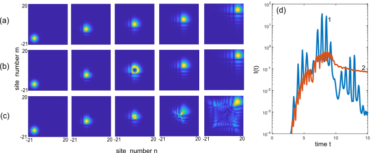
where $\psi_{n,m}(t)$ is the wave amplitude at site $(n,m)$ of the square lattice. As in Sec.III.B we consider a scattering potential of the form. $V_{n,m}(t)=R(t)V_{n,m}$ with a time-independent matrix $V_{n,m}$, defining the spatial shape of the local 2D scattering potential, and a modulation function $R(t)$ given by either $R(t)=A_{1}\exp(i\omega_{1}t)+A_{2}\exp(i\omega_{2}t)$ or $R(t)=A_{1}\cos(\omega_{1}t)+A_{2}\cos(\omega_{2}t)$ with incommensurate frequencies $\omega_{1}$ and $\omega_{2}$. Figure 4 illustrates the invisibility of the oscillating scattering potential when the modulation amplitude $R(t)$ is of the first type. The figure depicts the evolution of an initial Gaussian wave packet, propagating at an angle of 45^o with respect to the primitive vectors of the Bravais lattice, which is scattered off by the Gaussian-shaped 2D potential $V_{n,m}=V_{0}\exp(-n^{2}/w^{2}-m^{2}/w^{2})$. At initial time $t=0$ the wave packet is localized at the bottom left side of the lattice, far from the scattering region, and propagates along the main lattice diagonal toward the scattering region. Coupled equations (26) have been numerically solved using an accurate variable-step fourth-order Runge-Kutta method on a square lattice comprising $42\times 42$ sites; parameter values used in the simulations are $\kappa=1$, $V_{0}=25$, $w=2$, $\omega_{1}=10$, $\omega_{2}=2\sqrt{18}$, and $A_{1}=A_{2}=1$. The bandwidth of the lattice is $\Delta=8\kappa=8$. The initial condition is $\psi_{n,m}(0)=\mathcal{N}\exp[-(n+7)^{2}/9-(m+7)^{2}/9+i\pi(n+m)/2]$, where $\mathcal{N}$ is the normalization constant. Panels (a), (b) and (c) of Fig.4 show the temporal evolution of the wave packet in the absence of the scattering potential [Fig.4(a)], for a modulated NH scattering potential with $R(t)=A_{1}\exp(i\omega_{1}t)+A_{2}\exp(i\omega_{2}t)$ [Fig.4(b)], and for a modulated Hermitian scattering potential with $R(t)=A_{1}\cos(\omega_{1}t)+A_{2}\cos(\omega_{2}t)$ [Fig.4(c)]. The full dynamical evolution is shown in the movies 1,2 and 3 of the Supplemental Material Suppl . Clearly, in the latter case [Fig.4(c)] the potential is not invisible, and a large fraction of the incoming wave packet is scattered off by the oscillating Hermitian Gaussian-shaped potential. On the other hand, after the scattering event the wave packet in Fig.4(b) propagates as if the scattering potential were not present. This is clearly shown in Fig.4(d), which depicts the numerically-computed evolution of the error function $I(t)={\rm max}_{n,m}|\psi_{n,m}(t)-\tilde{\psi}_{n,m}|$ on a log scale, where $\psi_{n,m}(t)$ and $\tilde{\psi}_{n,m}(t)$ are the amplitudes at lattice site $(n,m)$ and at time $t$ with or without the scattering potential, respectively. Clearly, $I(t)\rightarrow 0$ as $t\rightarrow\infty$ is the signature of potential invisibility.

References

- (1) C.M. Bender, Rep. Prog. Phys. 70, 947 (2007).
- (2) N. Moiseyev, Non-Hermitian quantum mechanics, (Cambridge University Press, Cambridge, MA, 2011).
- (3) Y. Ashida, Z. Gong, and M. Ueda, Adv. Phys. 69, 3 (2020).
- (4) I. Kay and H. E. Moses, J. Appl. Phys. 27, 1503 (1956).
- (5) C. V. Sukumar, J. Phys. A 19, 2297 (1986).
- (6) A.K. Grant and J. L. Rosner, J. Math. Phys. 35, 2142 (1994).
- (7) J. Lekner, Am. J. Phys. 75, 1151 (2007).
- (8) S. Longhi, Phys. Rev. A 82, 032111 (2010).
- (9) S. Longhi, Opti. Lett. 35, 3844 (2010).
- (10) Z. Lin, H. Ramezani, T. Eichelkraut, T. Kottos, H. Cao, and D. N. Christodoulides, Phys. Rev. Lett. 106, 213901 (2011).
- (11) S. Longhi, J. Phys. A 44, 485302 (2011).
- (12) S. Longhi, Phys. Rev. A 81, 022102 (2010).
- (13) L. Feng, Y.-L. Xu, W. S. Fegadolli, M.-H. Lu, J. E. B. Oliveira, V. R. Almeida, Y.-F. Chen, and A. Scherer, Nature Mat. 12, 108 (2013).
- (14) S. Longhi and G. Della Valle, Ann. Phys. 334, 35 (2013).
- (15) A. Mostafazadeh, Phys. Rev. A 89, 012709 (2014).
- (16) A. Mostafazadeh, J. Phys. A 49, 445302 (2016).
- (17) M. Kulishov, H. F. Jones, and B. Kress, Opt. Express 23, 9347 (2015).
- (18) S. Longhi, EPL 117, 10005 (2017).
- (19) W.W. Ahmed, R. Herrero, M. Botey, Y. Wu, and K. Staliunas, Phys. Rev. Applied 14, 044010 (2020).
- (20) M. Sarisaman, Phys. Rev. A 95, 013806 (2017).
- (21) F. Loran and A. Mostafazadeh, Opt. Lett. 42, 5250 (2017).
- (22) A. Ruschhaupt, T. Dowdall, M. A. Simon, and J. G. Muga, EPL 120, 20001 (2017).
- (23) A. Ruschhaupt, M.A. Simon, A. Kiely, and J.G. Muga, J. Phys.: Conf. Ser. 2038, 012020 (2021).
- (24) A. Ruschhaupt, A. Kiely, M.A. Simon, and J.G. Muga, Phys. Rev. A 102, 053705 (2020).
- (25) K.G. Makris, A. Brandstötter, P. Ambichl, Z. H. Musslimani, and S. Rotter, Light Sci. Appl. 6, e17035 (2017).
- (26) S. Yu, X. Piao, and N. Park, Phys. Rev. Lett. 120, 193902 (2018).
- (27) E. Rivet, A. Brandstötter, K.G. Makris, H. Lissek, S. Rotter, and R. Fleury, Nature Phys. 14, 942 (2018).
- (28) A. F. Tzortzakakis, K. G. Makris, S. Rotter, and E.N. Economou, Phys. Rev. A 102, 033504 (2020).
- (29) K. G. Makris, I. Kresic, A. Brandstötter, and S. Rotter, Optica 7, 619 (2020).
- (30) A. Steinfurth, I. Krexic, S. Weidemann, M. Kremer, K.G. Makris, M. Heinrich, S. Rotter, and A. Szameit, Sci. Adv. 8 , eabl7412 (2022).
- (31) S.A.R. Horsley, M. Artoni, and G.C. La Rocca, Nature Photon.9, 436 (2015).
- (32) S. Longhi, EPL 112, 64001 (2015).
- (33) S.A.R. Horsley, C.G. King, and T.G. Philbin, J. Opt. 18, 044016 (2016).
- (34) S. Longhi, Opt. Lett. 41, 3727 (2016).
- (35) T.G. Philbin, J. Opt. 18, 01LT01 (2016).
- (36) S.A.R. Horsley, M. Artoni, and G.C. La Rocca, Phys. Rev. A 94, 063810 (2016).
- (37) C.G. King, S.A.R. Horsley, and T.G. Philbin, Phys. Rev. Lett. 118, 163201 (2017).
- (38) S.A.R. Horsley and S. Longhi, Am. J. Phys. 85, 439 (2017).
- (39) C. G. King, S. Horsley, and T. Philbin, J. Opt. 19, 085603 (2017).
- (40) S.A.R. Horsley and S. Longhi, Phys. Rev. A 96, 023841 (2017).
- (41) W. Jiang, Y. Ma, J. Yuan, G. Yin, W. Wu, and S. He, Laser & Photon. Rev. 11, 1600253 (2017).
- (42) D. Ye, C. Cao, T. Zhou, J. Huangfu, G. Zheng, and L. Ran, Nat. Commun. 8, 51 (2017).
- (43) S. Longhi, Phys. Rev. A 96, 042106 (2017).
- (44) S. Longhi, Opt. Lett. 42, 3229 (2017).
- (45) S. Longhi, Opt. Lett. 47, 4091 (2022).
- (46) S. Longhi, S.A. Horsley, and G. Della Valle, Phys. Rev. A 97, 032122 (2018).
- (47) Y. Zhang, J.H. Wu, M. Artoni, and G.C. La Rocca, Opt. Express 29, 5890 (2021).
- (48) S. Longhi, D. Gatti, and G. Della Valle, Phys. rev. B 92, 094204 (2015).
- (49) E. Papp and C. Micu, Low-dimensional Nanoscale Systems on Discrete Spaces (World Scientific, New Jersey, 2007).
- (50) D. C. Mattis, Rev. Mod. Phys. 58, 361 (1986).
- (51) T.B. Boykin, Eur. J. Phys. 25, 503 (2004).
- (52) D. N. Christodoulides, F. Lederer, and Y. Silberberg, Nature 424, 817 (2003).
- (53) I.L. Garanovich, S. Longhi, A.A. Sukhorukov, and Y.S. Kivshar, Phys. Rep. 518, 1 (2012).
- (54) F.T. Wall, Proc. Nat. Acad. Sci. 83, 5360 (1986).
- (55) F.T. Wall, Proc. Nat. Acad. Sci. 83, 5753 (1986).
- (56) S. Odake and R. Sasaki, J. Phys. A 44, 353001 (2011).
- (57) V. Spiridonov and A. Zhedanov, Ann. Phys. 237, 126 (1995).
- (58) A. A. Sukhorukov, Opt. Lett. 35, 989 (2010).
- (59) A. Szameit, F. Dreisow, M. Heinrich, S. Nolte, and A. A. Sukhorukov, Phys. Rev. Lett. 106, 193903 (2011).
- (60) S. Odake and R. Sasaki, J. Phys. A 48, 115204 (2015).
- (61) E. H. Lieb and D. W. Robinson, Commun. Math. Phys. 28, 251 (1972).
- (62) S. Longhi, Phys. Rev. A 77, 035802 (2008).
- (63) W. Li and L.E. Reichl, Phys. Rev. B, 60 , 15732 (1990).
- (64) M.V. Entin and M.M. Mahmoodian, EPL 84, 47008 (2008).
- (65) S. Longhi and G. Della Valle, Ann. Phys. 385, 744 (2017).
- (66) A. Schreiber, K. N. Cassemiro, V. Potocek, A. Gabris, P. J. Mosley, E. Andersson, I. Jex, and C. Silberhorn, Phys. Rev. Lett. 104, 050502 (2010).
- (67) A. Regensburger, C. Bersch, M. A. Miri, G. Onishchukov, D.N. Christodoulides, and U. Peschel, Nature 488, 167 (2012).
- (68) M. Wimmer, M. A. Miri, D. Christodoulides, and U. Peschel, Sci. Rep. 5, 17760 (2015).
- (69) X. Zhan, L. Xiao, Z. Bian, K. Wang, X. Qiu, B.C. Sanders, W. Yi, and P. Xue, Phys. Rev. Lett. 119, 130501 (2017).
- (70) L. Xiao, T. Deng, K. Wang, G. Zhu, Z. Wang, W. Yi, and P. Xue, Nature Phys. 16, 761 (2020).
- (71) S. Weidemann, M. Kremer, T. Helbig, T. Hofmann, A. Stegmaier, M. Greiter, R. Thomale, and A. Szameit, Science 368, 311 (2020).
- (72) K. Wang, T. Li, L. Xiao, Y. Han, W. Yi, and P. Xue, Phys. Rev. Lett. 127, 270602 (2021).
- (73) S. Longhi, Opt. Lett. 47, 2951(2022).
- (74) S. Weidemann, M. Kremer, S. Longhi, and A. Szameit, Nature Photon. 15, 576 (2021).
- (75) S. Weidemann, M. Kremer, S. Longhi, and A. Szameit, Nature 601, 354 (2022).
- (76) S. Longhi, Phys. Rev. B 105, 245143 (2022).
- (77) The Supplemental Material contains three movies (movie1.mp4, movie2.mp4, movie3.mp4), showing the temporal evolution of the wave packets corresponding to the cases of Fig.4(a), 4(b) and 4(c), respectively.