Non-intersecting path explanation for block Pfaffians and applications into skew-orthogonal polynomials
Abstract.
In this paper, we mainly consider a combinatoric explanation for block Pfaffians in terms of non-intersecting paths, as a generalization of results obtained by Stembridge. As applications, we demonstrate how are generating functions of non-intersecting paths related to skew orthogonal polynomials and their deformations, including a new concept called multiple partial-skew orthogonal polynomials.
Key words and phrases:
LGV lemma, Stembridge’s theorem, Pfaffians, orthogonal polynomials, skew-orthogonal polynomials2020 Mathematics Subject Classification:
15B52, 15A15, 33E201. Introduction
Enumerative combinatorics is always playing a fundamental role in mathematics and physics. Among these combinatorial objects, the theory of non-intersecting paths is an extremely useful theory with applications in counting tilings, plane partitions, and tableaux. In particular, the famous Lindström-Gessel-Vionnet (LGV) lemma states that the generating function of non-intersecting paths between vertex sets , where and have the same number of vertices, could be written as a determinant [24, 11]. This result has many applications such as non-intersecting random walks [17, 18], domino tiling models [8], dimer models [4], and so on. It turns out that the generating functions of non-intersecting paths are usually expressed in terms of structured determinants such as Hankel or Toeplitz determinants. Moreover, it has been shown in [26, 6] that the Hankel determinant of some special combinatorial numbers could be evaluated by using orthogonal polynomials, continued fraction and discrete integrable systems. Therefore, there is a unified relation between LGV lemma, integrable models, probability models, and orthogonal polynomials.
In [31], the author developed another algebraic tool—Pfaffian, to describe non-intersecting paths between a set of vertices to an interval. This combinatorial description for Pfaffian was also applied to count skew Young tableaux and plane partitions [27, 31]. A minor summation formula for Pfaffian [16] was given by using similar combinatorial technique, called the path switching involution in [21]. The minor summation formula is as an analogy of Cauchy-Binet formula for determinants, and it was applied to evaluate a certain Catalan-Hankel type Pfaffian
| (1.1) |
where are moments sequence related to little -Jacobi polynomials [15]. In fact, Pfaffian expression (1.1) is an important quantity in random matrix theory, especially for the characterization of symplectic invariant ensemble [25]. By realizing that (1.1) is a normalization factor for certain skew-orthogonal polynomials, various Catalan-Hankel type Pfaffians were computed by using skew-orthogonal polynomials under Askey-Wilson scheme in [29].
Inspired by these results, we attempt to give a unified frame between non-intersecting paths, Pfaffian formulas, and skew-orthogonal polynomials. It was known from [31] that the generating function of non-intersecting paths from could be written as a Pfaffian, namely,
| (1.2) |
where stands for all non-intersecting paths from an even-numbered vertex set to an interval and are some computable weights. Different from the Pfaffian formula considered in (1.1), we show that this generating function is related to another type of skew-orthogonal polynomials, which are related to orthogonal invariant ensemble in random matrix theory. Besides, if the vertex set , then its corresponding generating function could be expressed as an augmented Pfaffian
where is a weight function related to only. Since skew-orthogonal polynomials are only related to the even-ordered Pfaffian formula (1.2), we demonstrate that this augmented Pfaffian should be related to partial-skew-orthogonal polynomials proposed in [5].
In recent years, matrix-valued orthogonal polynomials play an important role in probability and combinatoric models such as hexagon tilings [14] and periodic Aztec diamond models [8]. Despite of block determinants, Pfaffians of skew symmetric block matrices were also proved to be useful in practice [22]. It was shown in [31] that the generating function for could be expressed as a block Pfaffian, with one block being all zeros. Here and are two sets of vertices and is an interval of vertices. Our first result is to give a non-intersecting path interpretation for block Pfaffians
| (1.5) |
We show that this Pfaffian could be expressed as the generating function of non-intersecting paths , where and are two sets of vertices and and are two intervals of vertices. Besides, we show that this generating function is related to a 2-component skew-orthogonal polynomials, which could be used to describe a non-intersecting random walk with two different sources. Moreover, a concept of multiple partial-skew-orthogonal polynomials is proposed if the number of vertices in and are odd. Furthermore, we extend formula (1.5) to a more general case, where we consider the paths from to . We show that this generating function could also be written as a block Pfaffian. We remark that in the reference [3], a non-intersecting path explanation for Pfaffians (1.5) was given, but it was shown by using Grassmann algebra in a cyclic digraph.
This paper is organized as follows. In Section 2, we recall the LGV lemma and show some applications. We connect the LGV lemma with several different orthogonal polynomials (including orthogonal polynomials on the real line and on the unit circle) and random walks (including discrete-time random walks and continuous-time random walks). In Section 3, we recall Stembridge’s results on the non-intersecting path explanation for Pfaffians. Their connections with skew-orthogonal polynomials and partial-skew-orthogonal polynomials are given. We show that this generating function is related to some random walk models as well. Thus we give a unified frame between non-intersecting paths, Pfaffian formulas and skew-orthogonal polynomials. We generalize Stembridge’s result in Section 4, where we consider paths from . Multiple skew-orthogonal polynomials are introduced by following this generating function, with some applications in random walks starting from different sources. Moreover, we introduce a new concept of multiple partial-skew-orthogonal polynomials from this generating function. In Section 5, non-intersecting paths between several vertex sets and intervals are considered. This is the most general case between vertex sets and intervals.
2. Lindström-Gessel-Vionnet theorem and applications into orthogonal polynomials
In this part, we give some brief reviews on the connections between Lindström-Gessel-Vionnet lemma and orthogonal polynomials. There have been numerous references about this topic, and please refer to [12, 21, 30, 28] and references therein.
Definition 2.1.
Let be a set of vertices, be a set of directed edges between vertices in , and represents an acyclic graph formed by and . We assume that the weight of each edge should be greater than zero.
Definition 2.2 ().
Let and be two vertices in . We use to denote the set of all paths from to in the graph .
Let be a path from to , that is, , then the weight of denoted by , is defined as the product of the weights of all edges on this path. Moreover, the weight between two vertices and is defined as .
Definition 2.3 (, ).
Let and be two sequences of vertices in , which are composed by points in an ascending order, namely, we assume that and . We denote by the set of all paths from to in the graph in the order , , …, and . Especially, we denote as the set of all non-intersecting paths from to .
Let be an -path starting from to , where is a path from to . The weight of is defined to be . Moreover, if we count the weight for all paths from to , then we have
In general, we refer this weight function as the generating function of all paths from to , and denote it as GF. For non-intersecting paths, we have GF.
Definition 2.4 (-Compatible).
If and are ordered sets of vertices in a graph , then is said to be D-compatible with in the graph if and only if for any in and any in , every path intersects with every path .
Now, we could formally state the LGV lemma.
Theorem 2.5 ([24, 11, 31]).
Let and be two ordered -tuples of vertices in an acyclic directed graph . If and are D-compatible, then
| (2.1) |
In literatures, there have been many applications of Lindstörm-Gessel-Vionnet lemma. For example, it has been applied to some tiling problem and random growth models [17, 8]. Originally, non-intersecting paths arose in matroid theory [24], which was later used to count tableaux and plane partitions [11]. In the references mentioned above, there is a specialized binomial determinant related to Toeplitz (respectively Hankel) determinant and orthogonal polynomials on the unit circle (respectively real line). Here we start with a non-intersecting random walk model and demonstrate how LGV lemma works in the random walk models and orthogonal polynomial theory.
Let’s consider independent simple random walks starting from positions at , and ending at positions at with conditions and . There are two different models related to this setting. One is a continuous-time model called non-intersecting Brownian motion with configuration [1, 9]. We first assume to be independent standard Brownian motions with transition probability
which indicates the probability from to within time . Moreover, let’s assume that is a admissible configuration. In this case, non-intersecting means that for all . According to the Karlin-McGregor’s theorem [19], the conditional probability density function (PDF) for passing through at time and ending at , given the starting point and the total duration of , is expressed by
| (2.2) |
This result could be also recognized as an application of LGV lemma, where could be viewed as the generating function from to , and could be viewed as the generating function from to . To calculate the conditional probability of event , we normalize it by dividing a normalization factor for reaching from within the total time of . In fact, this normalization factor is given by , where is a normal distribution with mean zero and variance . Therefore, the conditional probability of the event could expressed by
In fact, the PDF (2.2) induces a bi-orthogonal system. We demonstrate this result in the following proposition.
Proposition 2.6.
If we denote and , then we could introduce moments as
Moreover, functions
and
are orthogonal to each other with the uniform measure. In other words, we have
where
This is a general bi-orthogonal system [2]. If we consider confluent starting and ending point, then we could define multiple orthogonal polynomials and multiple orthogonal polynomials of mixed type [7]. To be precise, let’s consider a confluent case where non-intersecting Brownian motions start from different points with multiplicity for , and end at different points with multiplicity for , such that . Under this circumstance, we have the following proposition for multiple orthogonal polynomials of mixed type.
Proposition 2.7.
Let’s denote for and and for and , where and . We define moments of mixed type by
for In this case, multiple orthogonal polynomials of mixed type could be written as
where
Moreover, these polynomials satisfy the following mixed orthogonality
Another application is to consider a discrete-time random walk, defined in the configuration space . At each discrete time step, the simple random walk increase or decrease by one step with equal probability. If we denote and for all , and assume that all paths don’t intersect, then the number of all non-intersecting paths is given by a binomial determinant [20, 10]
Such a model is sometimes referred to as vicious random walkers which means that the walkers can not be in the same position at each discrete step. It was shown in [10] that this binomial determinant is related to symmetric Hahn polynomials. However, the following proposition demonstrates that such a binomial determinant could also be related to a Toeplitz determinant and orthogonal polynomials on the unit circle (OPUC).
Proposition 2.8.
([12] with a correction) The binomial coefficient could be written by a residue formula
where denotes a unit circle. Moreover, if for , then the binomial determinant could be expressed as a Toeplitz determinant .
3. Stembridge’s results on Pfaffians and applications into skew-orthogonal polynomials
In [31], Stembridge generalized the result of Lindström-Gessel-Viennot, by considering non-intersecting paths from a set of vertices to an ordered subset , whose number of vertices is indefinite. In this section, let’s assume that is a finite sequence of vertices in .
Definition 3.1 (, , ).
Let be the set of all paths from to any , be the r-tuple set of paths where , and be the non-intersecting paths in .
Definition 3.2 ().
refers to the generating function of all non-intersecting paths from to in the graph . Literally, we can write .
Especially, if , which is a single vertex, then
| (3.1) |
If , then according to LGV theorem, we have
| (3.2) |
where sgn is a sign function defined by
Remark 3.3.
The generating function for 2-points (3.2) naturally induces a skew-symmetric inner product. If we define
| (3.3) |
then this inner product is skew symmetric, i.e. we have . Moreover, if we take
then we see that
It was found by Stembridge that could be written as a Pfaffian, whose elements are given by (3.1) and (3.2). To this end, let’s introduce the concept of 1-factor, and the graphic definition of Pfaffians.
Definition 3.4 (1-Factor).
Let . For each perfect matching for these vertices, the set of all pairings is called a 1-factor. Denote the set of all 1-factors for as . Specifically, if the set consists of the first consecutive natural numbers, then the set of 1-factors can be simply denoted as .
For example, for a set , the perfect matching is a 1-factor in .
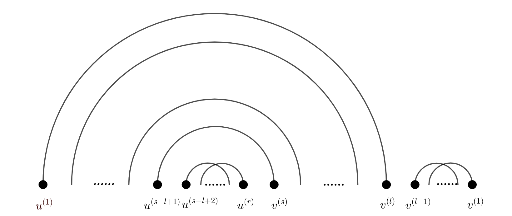
Definition 3.5 (Crossing Number).
For any 1-factor for the set , if we align vertices in a straight line with order , and connect the paired ones with curves above the line, then the number of intersections of these curves is defined as the crossing number, denoted by . The sign of is defined as .
Definition 3.6 (Definition of Pfaffians).
If is a skew symmetric matrix of order such that , then we can define the Pfaffian of by
| (3.4) |
3.1. The generating function for non-intersecting paths from
The following result was given by Stembridge in [31, Thm. 3.1].
Theorem 3.7.
Remark 3.8.
It should be remarked that if we consider the generating function for non-intersecting paths from to , then we have the expression
where
and could be computed by above 1-vertex and 2-vertex formulas for any .
3.2. The generating function of non-intersecting paths from
In this part, let’s assume and with .
Definition 3.9 ().
is defined as a union of vertices and , where and are disjoint, and all vertices are arranged such that every in precedes vertices in .
Definition 3.10 ().
is defined as the set of all non-intersecting paths , where for , ; while for , .
Theorem 3.11 ([31] with a supplement statement).
Let and be sequences of vertices in the acyclic directed graph , and suppose is a totally ordered subset of such that and are -compatible. If is even, then
where
| (3.5) |
Moreover, if is odd, then
where
and matrices and are given by (3.5).
Proof.
Here we give a proof when is odd, which is omitted in Stembridge’s paper. We assume that there is an auxiliary vertex added in the graph . In order to satisfy -compatibility, we might as well assume that this vertex follows all vertices in and . Furthermore, we require that weights of to itself is , and to other vertices are zero. Let’s denote , , then one could show that
which gives the result. ∎
It should be remarked that the Theorem 3.11 comprises previous results in Theorem 2.5 and Theorem 3.7. If is an empty set, then it degenerates to Theorem 3.7, while if is an empty set and , then it degenerates to the LGV lemma. Therefore, we want to generalize Stembridge’s result to consider combinatoric explanations for full block Pfaffians. Before that, a comparison to Ishikawa-Wakayama’s result is made to show the strength of Stembridge’s method.
3.3. A comparison to Ishikawa-Wakayama’s result
In [16, Theorem 4.3], Ishikawa and Wakayama obtained similar results to Theorem 3.7, which reads
In the above formula, is a set of points consisting of an even number of elements, is a finite set of even-number vertices, and represents the set of all subsets of containing exactly elements. Moreover, is a skew-symmetric matrix and is the submatrix of obtained by picking up the rows and columns indexed by S, and .
To relax the condition of -compatibility, Ishikawa and Wakayama imposed an additional condition that the set of vertices should be finite and the number of vertices should be even. When and are -compatible, we can get the same result stated as in Theorem 3.7. Moreover, Ishikawa and Wakayama generalized Theorem 3.11 to [16, Theorem 4.4], where the -compatible condition is relaxed. For both and being even, , we have
where
Although the results of Stembridge and Ishikawa-Wakayama are both non-intersecting path explanations for Pfaffians, Stembridge derived the general generating function from to by using the 1-vertex generating function (3.1) and 2-vertex generating function (3.2), while Ishikawa-Wakayama derived the general generating function by the weight between points in and , which contains more imformation between and . This is the reason why -compatibility could be relaxed. Furthermore, Ishikawa-Wakayama’s proof avoided internal pairings between points in , which made it easier to find a map to offset all intersecting paths. Since we don’t want to make any constraints on the terminal interval , we still adopt Stembridge’s method in the following sections.
3.4. Application of Stembridge’s theorem
There have been numerous application of Stembridge’s graphic explanation for Pfaffians. In [31, 27], it was used to count skew Young tableaux and the enumeration of plane partitions, and later it was used to demonstrate a minor summation formula for Pfaffian in [16]. In recent years, a fusion of combinatorial technique and statistical physics leads to more applications of Stembridge’s result. For example, Theorem 3.7 was used in a vicious random walker problem without return [10], and Theorem 3.11 was used in a free-boundary lozenge tiling problem [4, Section 4] where some triangular holes in the lattices were imposed. In this part, we demonstrate how to introduce skew-orthogonal polynomials by considering non-intersecting Brownian motions and applications of Stembridge’s results.
Let’s first consider independent simple random walks starting from as in Section 2. If we consider a continuous-time non-intersecting Brownian motion in the configuration space , then it is known that at an arbitrary time , the distribution of arrival points at could be formulated by
| (3.6) |
with a normalization factor . If is even, then could be written by
where
Moreover, if is odd, then
with . It should be noted that the element in this Pfaffian coincide with the formula in the skew-symmetric inner product (3.3). Moreover, we have the following proposition.
Proposition 3.12.
Let’s define monic functions
where , , and and are two column vectors admitting the forms for . Moreover, satisfy skew orthogonality relations
It should be remarked that there are only involved under the frame of skew-orthogonal polynomials. To have a clear understanding of , partial-skew-orthogonal polynomials should be introduced and we have the following proposition.
Proposition 3.13.
If we define monic functions
where , and . Moreover, are determined by the following relations
4. Non-intersecting path explanations for block Pfaffians and applications
In this section, we generalize Stembridge’s theorem and obtain a block matrix representation for generating function of non-intersecting paths. We assume that these paths should start from and end at several different sets of vertices.
4.1. Pfaffian representations for
To give a Pfaffian representation for paths , we need to introduce the separation of a graph.
Definition 4.1 (-separated).
We call vertex sets and to be -separated if paths from to and those from to are non-intersecting.
Definition 4.2 ().
If a graph is -separated, then represents all non-intersecting paths without any path from . Moreover, paths should be consecutive; that is, if there is a path from , then we must have and so on, until that is matched over.
Again, we assume that and . If is even, then we use (respectively ) to denote the number of paths from and are both even (respectively both odd). Here we don’t have the case where the number of paths from is even, and that from is odd. Otherwise there will be some paths from , which is contradicted with -separated . On the other hand, if is odd, then we use (respectively ) to represent that there are even (respectively odd) paths from and odd (respectively even) paths from . Let’s denote weight matrices
and column vectors and .
Theorem 4.3.
Let and be sequences of vertices in an acyclic directed graph . Assume that and are totally ordered subsets of , such that and are -compatible and -separated. If is even, then we have
| (4.3) |
and
| (4.8) |
On the other hand, if is odd, then
| (4.12) |
and
| (4.16) |
Proof.
Let’s prove the equation (4.3), and (4.8)-(4.16) could be similarly verified. This proof is based on the path switching involution for non-intersecting paths, and is divided into three steps.
(1) Expanding the Pfaffian as a summation of configurations. By expanding (4.3), we have
where belongs to the set . We recognize this formula as a product of path weights by rewriting it as
| (4.19) |
where is a configuration such that
-
•
If , then ;
-
•
If , then , , while and don’t intersect;
-
•
If , then , , while and don’t intersect.
We call these three conditions as the configuration conditions.
(2) Finding a sign-reversing involution to offset the intersecting paths. To make the RHS in (4.19) represent the summation of weights for all non-intersecting paths, we intend to show that there exists an involution which can offset the intersecting term. Since the graph is -separated, we know that if there are paths intersected, then the intersecting point belongs to or for some and . We show the first case and the latter could be similarly verified. Let’s find the smallest intersecting point 111We call an intersecting point the smallest if it is the first intersecting point starting from . If there isn’t any intersecting point in , then we find it in , and so on.(the biggest intersecting point in the latter case). Among the paths passing through , we assume that and are the two paths which admit two smallest indices. Thus we could construct an involution
where we define paths and as
and the other paths remain the same. At the same time, is obtained by interchanging and in . Next, we show that is still a configuration, and is sign-reversing.
To prove this, we first demonstrate that is still in the summation (4.19), which is equivalent to verify that satisfies configuration conditions. Since the paths except and remain the same, it is necessary to consider cases in which only contain or . If , then we have , implying that . Therefore, as is obtained by interchanging and in , it is known that and as required. To show that and do not intersect, we verify it by contradiction. Assume that and intersect with each other at some point, then the intersection point could only be behind the smallest . However, since is the same as after the point , it means that and intersect, which leads to a contradiction with . On the other hand, if , then , and therefore . From this fact, we know that as required. To show the map is sign-reversing, by making use of -compatibility, we know that for any satisfying , must intersect with and . Therefore, by using [31, Lem. 2.1], we can deduce that this involution mapping is sign-reversing.
(3) Simplification of the configuration. After offsetting intersecting terms, only non-intersecting terms are left. Therefore, (4.19) could be rewritten as the non-intersecting part of
| (4.20) |
where
Moreover, by realizing
we know that (4.20) represents the weight of all non-intersecting paths from , and there are even paths from and even paths from . ∎
Let’s end with an example. If and , then it is known that
where the first term represents the weight of non-intersecting paths from and , and the rest terms represent the weight of non-intersecting paths from and .
4.2. Applications of block Pfaffians and multiple skew-orthogonal polynomials
In this subsection, we show some applications of this block Pfaffians, which correspond to the multiple skew-orthogonal polynomial theory.
We start with the probability density function given by (3.6). If we consider there are only two starting points named and , and there are paths from for , then we have a confluent form for the PDF. By noting that
where , we know that the normalization factor in this case could be written as
| (4.21) |
if is even. Here we note that the partition function is in the form of equation (4.3). Moreover, in the above notations, we have
This normalization factor induces the following definition of multiple skew-orthogonal functions.
Proposition 4.4.
Let’s denote , , and . If is odd, then we could define functions
and they satisfy the following multiple skew orthogonality 222Here and is the unit vector whose th element is , and the others are . For example, .
where is given by (4.21).
Instead, inspired by the generating function in the forms (4.12) and (4.16), we could introduce a new concept of multiple partial-skew-orthogonal polynomials. Namely, we could define another family of functions and to replace and when is odd.
Proposition 4.5.
For being odd, we could define
Moreover, these functions satisfy the following partial-skew orthogonality
As mentioned in [23], the advantage of partial-skew-orthogonality mainly lie in the existence of Pfaffian formula for odd order. We hope that these multiple partial-skew-orthogonal polynomials would be useful in the future study of classical integrable systems, including spectral transformations and corresponding Pfaffian -functions.
5. Generating functions for non-intersecting paths between several sets and intervals
In this section, we consider non-intersecting paths between several sets and intervals. To this end, we consider different sets of vertices and and different intervals of vertices and . Here we assume that each has vertices labelled by and each has vertices labelled by . Moreover, we should assume that and are both totally ordered sets of vertices.
Definition 5.1 ().
For different vertex sets and different vertices intervals , let’s define as direct sums of sets and intervals by inserting into , and each vertex in precedes those in for .
For example, if there are two sets of vertices and two intervals , then
Moreover, we can define is a specific element in with ordering . Given this , we could define by replacing by for , and replacing by for . For example, if we define
then we have
With this setting, we could define non-intersecting paths between several sets and intervals.
Definition 5.2 ().
Given as a specific ordering, let’s denote as all disjoint paths where vertices in go to and for any and , while vertices in go to the rest of . We further assume that the number of paths from to and those from to are both even.
Definition 5.3 (Continuity of 1-Factors).
A 1-factor
| (5.1) |
is said to be continuous if it satisfies the following two conditions: 1. If there is some paired with , then is paired with , then must be paired with , until all elements in or are fully paired, and the rest in and are internally paired separately (see Figure 2.a) ; 2. Under the order , if and are adjacent, and is paired with , then is paired with (see Figure 2.b). This is also true for and .
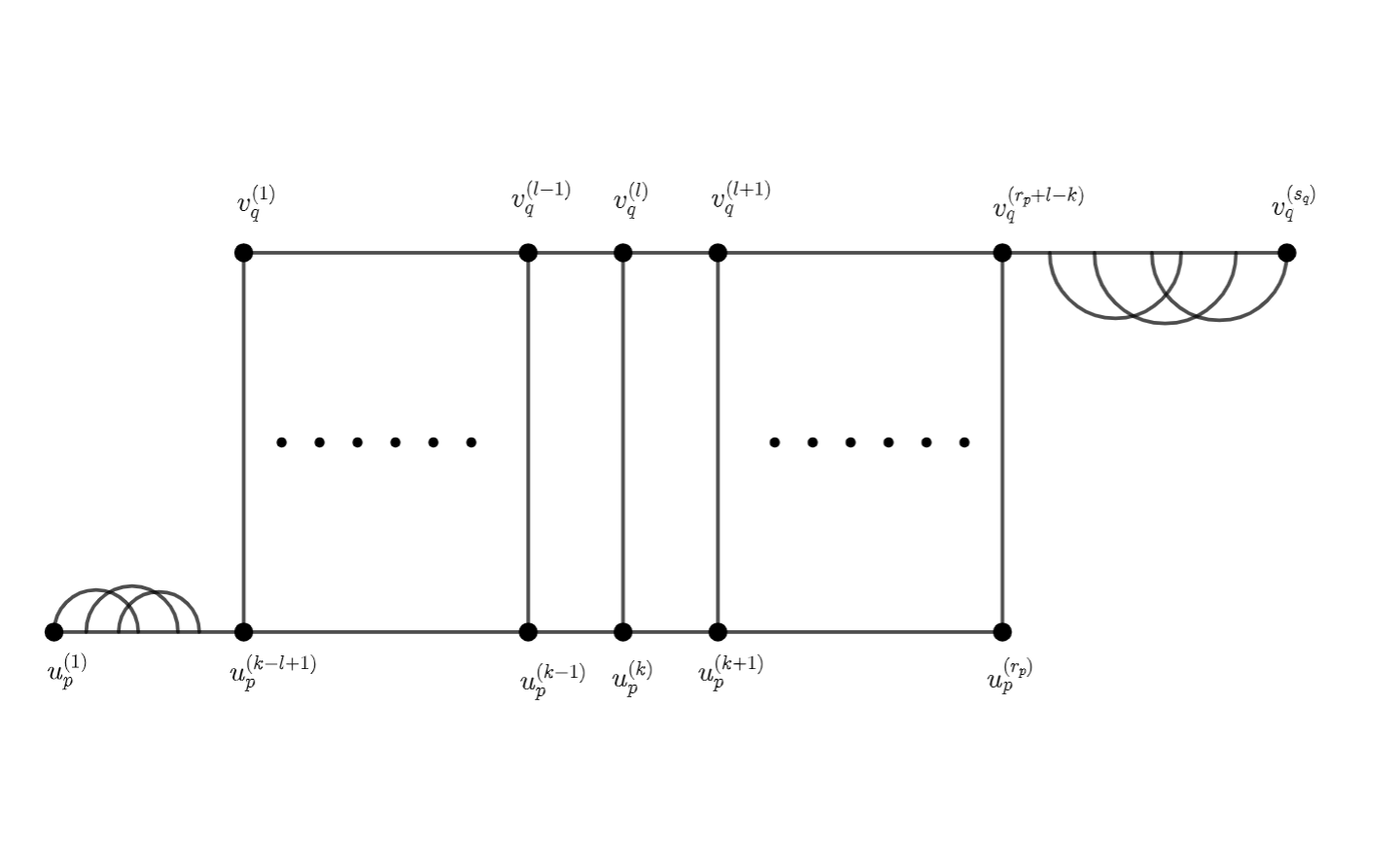
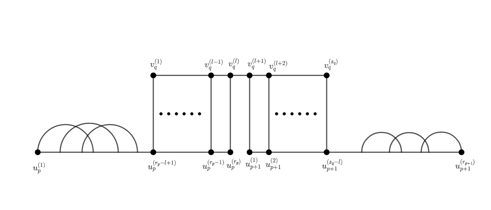
It should be noted that a continuous 1-factor could be divided into three parts. Namely, for any , we have
where , , , and ,. Here means a continuous pairing between and , and (respectively ) means a pairing between vertices in (respectively in ). We denote all continuous 1-factors as a set .
Here we remark that and could not be merged into one vertex set, since there could be paths from and from . These paths are different.
Definition 5.4 (-separated).
Two ordered sets of vertices and are -separated if any path from to does not intersect with any path starting from , and any path from to does not intersect with any path to . Moreover, and any path from to does not intersect with any path from to for all and .
Theorem 5.5.
Let and be sequences of vertices in the acyclic directed graph , and assume that is even. If for any , , are totally ordered subsets of , such that and are -compatible and -separated. Then
| (5.4) |
where
Proof.
First, we know that the right hand side of equation (5.4) could be expanded as
according to the formula (3.4), where the summation is over all continuous 1-factors (5.1). Moreover, we could recognize this formula as a product of path weights and rewrite it as
| (5.7) |
where and are a set of paths, , , and is an -tuple configuration such that
-
•
If ,then ;
-
•
If ,then ,,while and don’t intersect;
-
•
If ,then ,,while and don’t intersect.
Then, we seek for a sign-reversing involution to offset the intersecting paths. Since the graph is -separated, we know that if paths intersect, then the intersecting point belongs to or for some and . Similar to the proof in Theorem 4.3, we find the smallest intersection point 333In this case, we find the smallest intersection point starting from paths in . If there is an intersection point in , then we find it from paths starting from and the rest is the same with the case in Theorem 4.3. If there isn’t any intersection point in , then we find it in , and so on., and assume that and are the two whose subcripts (priority) and supercripts (followed) are the smallest. Thus, we could construct an involution
where
and the rest paths remain invariant. Using the method shown in Theorem 4.3, we can verify that this map is a sign-reversing involution by the property of -separated graph.
By using the sign-reversing involutions to cancel the intersection terms, we find that only configurations containing continuous 1-factors are left. As we divide the continuous 1-factor into 3 parts, (5.4) could be rewritten as the non-intersecting part of
| (5.8) |

Moreover, by realizing
we know that (5.8) represents , and there are even paths from and even paths from .
∎
Acknowledgement
We would like to thank the referee for useful comments. This work is partially funded by grants (NSFC12101432, NSFC12175155).
References
- [1] J. Baik and Z. Liu. Discrete Toeplitz/Hankel determinants and the width of non-intersecting processes. Int. Math. Res. Not., 20 (2014), 5737-5768.
- [2] A. Borodin. Biorthogonal ensembles. Nucl. Phys. B, 536 (1998) 704-732.
- [3] S. Carrozza and A. Tanasa. Pfaffians and nonintersecting paths in graphs with cycles: Grassmann algebra methods. Adv. Appl. Math., 93 (2018), 108-120.
- [4] M. Ciucu and C. Krattenthaler. The interaction of a gap with a free boundary in a two dimensional dimen system. Commun. Math. Phys., 302 (2011), 253-289.
- [5] X. Chang, Y. He, X. Hu and S. Li. Partial-skew-orthogonal polynomials and related integrable lattices with Pfaffian -function. Comm. Math. Phys., 364 (2018) 1069-1119.
- [6] X. Chen, X. Chang, J. Sun, X. Hu and Y. Yeh. Three semi-discrete integrable systems related to orthogonal polynomials and their generalized determinant solutions. Nonlinearity, 28 (2015), 2279-2306.
- [7] E. Daems and A. Kuijlaars. Multiple orthogonal polynomials of mixed type and non-intersecting Brownian motions. J. Approximation Theo., 146 (2007), 91-114.
- [8] M. Duits and A. Kuijlaars. The two-periodic Aztec diamond and matrix valued orthogonal polynomials. J. Eur. Math. Soc., 23 (2021), 1075-1131.
- [9] P. Forrester, S. Majumdar and G. Schehr. Non-intersecting Brownian walkers and Yang-Mills theory on the sphere. Nuclear Phys. B, 844 (2011), 500-526.
- [10] P. Forrester and T. Nagao. Vicious random walkers and a discretization of Gaussian random matrix ensembles. Nuclear Phys. B, 620 (2002), 551-565.
- [11] I. Gessel and G. Viennot. Binomial determinants, paths, and hook length formulae. Adv. Math., 58 (1985), 300-321.
- [12] R. Gharakhloo and K. Liechty. Bordered and framed Toeplitz and Hankel determinants with applications in integrable probability. arXiv: 2401.01971.
- [13] R. Gharakhloo and N. Witte. Modulated bi-orthogonal polynomials on the unit circle: the and systems. Constr. Approx., 58 (2023), 1-74.
- [14] A. Groot and A. Kuijlaars. Matrix-valued orthogonal polynomials related to hexagon tilings. J. Approximation Thoery, 270 (2021), 105619.
- [15] M. Ishikawa, H. Tagawa and J. Zeng. Pfaffian decomposition and a Pfaffian analogue of -Catalan Hankel determinants. J. Combin. Theory Ser. A., 120 (2013), 1263-1284.
- [16] M. Ishikawa and M. Wakayama. Applications of minor summation formula III, Plücker relations, lattice paths and Pfaffian identities. J. Combin. Theory Ser. A., 113 (2006), 113-155.
- [17] K. Johansson. Non-intersecting paths, random tilings and random matrices. Probab. Theory Related Fields., 123 (2002), 225-280.
- [18] K. Johansson. Non-colliding Brownian motions and the extended tacnode process. Comm. Math. Phys., 319 (2013), 231-267.
- [19] S. Karlin and J. McGregor. Coincidence probabilities. Pacific J. Math., 9 (1959), 1141-1164.
- [20] C. Krattenthaler, A. Guttmann and X. Viennot. Vicious walkers, friendly walkers and Young tableaux. II. With a wall. J. Phys. A 33 (2000), 8835.
- [21] C. Krattenthaler. Lattice path enumeration. Discrete Math. Appl., CRC Press, Boca Raton, FL, 2015, 589-678.
- [22] S. Li, B. Shen, J. Xiang and G. Yu. Multiple skew orthogonal polynomials and 2-component Pfaff lattice hierarchy. Ann. Henri Poincaré, https://doi.org/10.1007/s00023-023-01382-2.
- [23] S. Li and G. Yu. Christoffel transformations for (partial-)skew-orthogonal polynomials and applications. Adv. Math., 436 (2024), 109398.
- [24] B. Lindström. On the vector representations of induced matroids. Bull. London Math. Soc., 5 (1973), 85-90
- [25] M. Mehta and R. Wang. Calculation of a certain determinant. Comm. Math. Phys., 214 (2000), 227-232.
- [26] Y. Nakamura and A. Zhedanov. Special solutions of the Toda chain and combinatorial numbers. J. Phys. A, 37 (2004), 5849-5862.
- [27] S. Okada. On the generating functions for certain classes of plane partitions. J. Combin. Theory Ser. A, 51 (1989), 1-23.
- [28] B. Sagan. The symmetric group. GTM Vol. 203, Springer, 2001.
- [29] B. Shen, S. Li and G. Yu. Evaluations of certain Catalan-Hankel Pfaffians via classical skew orthogonal polynomials. J. Phys. A, 54 (2021) 264001.
- [30] R. Stanley. Enumerative combinatorics, Vol.2, Cambridge University Press, 1999.
- [31] J. Stembridge. Nonintersecting paths, Pfaffians, and plane partition. Adv. Math., 83 (1990), 96-131.