Non-linear PDEs approach to statistical mechanics of Dense Associative Memories
Abstract
Dense associative memories (DAM), are widespread models in artificial intelligence used for pattern recognition tasks; computationally, they have been proven to be robust against adversarial input and theoretically, leveraging their analogy with spin-glass systems, they are usually treated by means of statistical-mechanics tools. Here we develop analytical methods, based on nonlinear PDEs, to investigate their functioning. In particular, we prove differential identities involving DAM’s partition function and macroscopic observables useful for a qualitative and quantitative analysis of the system. These results allow for a deeper comprehension of the mechanisms underlying DAMs and provide interdisciplinary tools for their study.
Keywords:
-spin, Statistical mechanics, Burgers hierarchy, Nonlinear systems, Mean-field theory, PDE1 Introduction
Artificial intelligence (AI) is rapidly changing the face of our society thanks to its impressive abilities in accomplishing complex tasks and extracting information from non-trivially structured, high-dimensional datasets. The successful applications of modern AI range from hard sciences and technology to more practical scenarios (e.g. medical sciences, economics and finance, and many daily tasks). Its important success is primarily due to the ascent of deep learning LeCun2015 ; Schmidhuber2015 , a set of semi-heuristic techniques consisting in stacking together several minimal building blocks in complex architectures with extremely-high learning performances. Despite its success, a rigorous theoretical framework guiding the development of such machine-learning architectures is still lacking. In this context, statistical mechanics of complex systems offers ideal tools to study neural network models from a more theoretical (and rigorous) point of view, thus drawing a feasible path which makes AI less empirical and more explainable.
In statistical mechanics, a primary classification of physical systems is the following. On the one side, we have simple systems, which are essentially characterized by the fact that the number of equilibrium configurations does not depend on the system size . A paradigmatic (mean-field) realization of this situation is the Curie-Weiss (CW) model, in which all the spins , , making up the system interact pairwisely by a constant, positive (i.e. ferromagnetic) coupling . Below the critical temperature, in fact, the system exhibits ordered collective behaviors, and the equilibrium configurations of the system are characterized by only two possible values of the global magnetization (which are further related by a spin-flip symmetry for each ). On the opposite side, we have complex systems, in which the number of equilibrium configurations increases according to an appropriate function of the system size due to the presence of frustrated interactions mezard1988spin . The prototypical example of mean-field spin-glass is the Sherrington-Kirkpatrick (SK) model sherrington1975 , in which the interaction strengths between the spin pairs are i.i.d. Gaussian variables. With respect to simple systems, spin-glass models exhibit a richer physical and mathematical structure, as shown by the presence of the spontaneous replica-symmetry breaking and an infinite number of phase transitions (e.g. see Parisi1979rsb1 ; Parisi1979rsb2 ; Parisi1980rsb3 ; Parisi1980sequence ; mezard1984replica ; guerra2003broken ; ghirlanda1998general ; talagrand2000rsb ) as well as the ultrametric organization of pure states (e.g. see panchenko2010ultra ; panchenko2011ultra ; panchenko2013parisi ). Statistical mechanics of spin glasses has acquired a prominent role during the last decades due to its ability to describe the equilibrium dynamics of several paradigmatic models for AI, in particular thanks to the work by Amit, Gutfreund, and Sompolinsky amit1985 for associative neural networks. For our concerns, the relevant ones are the Hopfield model hopfield1982hopfield ; pastur1977exactly and its -spin extensions, the Dense Associative Memories (DAMs) Krotov2016DenseAM ; Krotov2018DAMS ; AD-EPJ2020 , exhibiting features which are peculiar both of ferromagnetic (simple) and spin-glass (complex) systems. In these models, the interactions between the spins are designed in order to store “information patterns”, each encoded by binary vectors of length and denoted by , with and is a Rademacher random variable for any and ; the -th pattern is said to be stored if the configuration is an equilibrium state and the relaxation to this configuration, starting from a relatively close one (i.e. a corrupted version of ), is interpreted as the retrieval of that pattern. The Hamilton function (or the energy in physics jargon) of these systems can be expressed as
where is the interaction order (for the Hopfield model , while for the DAMs) and is the so-called Mattis magnetizations measuring the retrieval of the -th pattern. It has been shown that the number of storable patterns scales, at most, as a function of the system size, more precisely, , where depends on the interaction order and is referred to as critical storage capacity baldi1987number ; bovier2001spin . By a statistical-mechanics investigation of these models one can highlight the macroscopic observables (order parameters) useful to describe the overall behavior of the system, namely to assess whether it exhibits retrieval capabilities, and the natural control parameters whose tuning can qualitatively change the system behavior; such knowledge can then be summarized in phase diagram.
Regarding the methods, statistical mechanics offers a wide set of techniques for analyzing the equilibrium dynamics of complex systems, and in particular to solve for their free-energy. Historically, the first method (which was applied to the SK model and the Hopfield model amit1985 ; steffan1994replica ) is the replica trick, which – despite being straightforward and effective – is semi-heuristic and suffers from delicate points, see for example tanaka2007moment . Alternative, rigorous approaches were developed during the years and, among these, the relevant one for our concerns is Guerra’s interpolating framework. In this case, we can take advantage of rigorous mathematical methods by applying sum rules guerra2001sum or by mapping the relevant quantities (the free energy or the model order parameters) of the statistical setting to the solutions of PDE systems. Indeed, differential equations involving the partition functions (or related quantities) of thermodynamic models have been extensively investigated in the literature, see for example agliari2012notes ; barra2013mean ; barra2008mean ; barra2010replica ; barra2014proc ; Moro2018annals ; AMT-JSP2018 ; Moro2019PRE ; ABN-JMP2019 ; fachechi2021pde ; AAAF-JPA2021 . In particular, they allow us to express the equation of state (or the self-consistency equations) governing the equilibrium dynamics of the system in terms of solutions of non-linear differential equations, and to describe phase transition phenomena as the development of shock waves, thus linking critical behaviours to gradient catastrophe theory Barra2015Annals ; DeNittis2012PrsA ; Giglio2016Physica ; Moro2014Annals . In a recent work fachechi2021pde , a direct connection between the thermodynamics of ferromagnetic models with interactions of order and the equations of the Burgers hierarchy was established by linking the solution of the latter as the equilibrium solution of the order parameter of the former (i.e. the global magnetization ). In the present paper, we extend these results to complex models, in particular to the Hopfield model and the DAMs.
The paper is organised as follows. In Section 2, we introduce the relevant tools for our investigations, in particular Guerra’s interpolating scheme for the PDE duality. In Section 3, as a warm up, we review some basic results about the -spin ferromagnetic models. In Section 4, we extend our results to the Derrida models (constituting the spin extension of the SK spin glass) derrida1981rem . In Section 5, we merge our results in a unified methodology for dealing with the DAMs, especially in the so-called high storage limit, and re-derive the self-consistency equations for the order parameters by means of PDE technology.
2 Generalities and notation
In this Section, we present the thermodynamic objects we aim to study. We start with a system made up of spins whose configurations are the nodes of a hypercube and interacting via a suitable tensor of order . The Hamilton functions of the system we will consider in this paper are of the form
| (1) |
where is a normalization factor ensuring the linear extensivity of the energy with the system size. Once the Hamiltonian is fixed, we introduce the partition function in the usual Boltzmann-Gibbs form. Thus, given the level of thermal noise of the system, the partition function is defined as
| (2) |
For simple systems, the partition function can be computed exactly for any coupling matrix. As is standard in statistical mechanics, it is convenient to compute intensive quantities which are well-defined in the thermodynamic limit . Since the partition function is a sum of contribution, it is sufficient to take the intensive logarithm of the partition function, i.e.
which is the intensive statistical pressure (which is, apart for a factor , the usual free energy) of the system. However, when dealing with spin-glass systems, the coupling tensor is a multidimensional random variable, thus the partition function defines a random measure on the configuration space. For good enough probability distributions of the coupling matrix, the intensive logarithm of the partition function is expected to converge to its expectation value in the thermodynamic limit by virtue of self-averaging theorems ShcherbinaPastur-JSP1991 ; Bovier-JPA1994 , so it is natural to consider the quenched intensive pressure associated to the partition function (2), which is defined as
| (3) |
where denotes the average over the quenched disorder (we stress that, in this case, the free energy does not depend any longer on the coupling matrix because of the average operation).
Rather than working with the quantity (2), we will use as a fundamental object Guerra’s interpolated partition function and its associated interpolating intensive pressure. For instance, for spin-glass systems we would have
| (4) |
where denotes the interpolating Hamiltonian satisfying the properties that, at and , it recovers the Hamiltonian (1) times , and at and it corresponds to an exactly-solvable -body system, namely a system where spins interact only with an external field that has to be set a posteriori. The interpolating parameters and are interpreted, in a mechanical analogy, as spacetime coordinates with suitable dimensionality.
The interpolating structure (4) implies a generalized measure, whose related Boltzmann factor is
| (5) |
Thus, for an arbitrary observable in the configuration space , we can introduce the Boltzmann average induced by the partition function (4) as
| (6) |
Usually, in spin-glass systems, the quenched average is performed after taking the Boltzmann expectation values on the -replicated space , which is naturally endowed with a random Gibbs measure corresponding to the partition function . Given a function , the Boltzmann average in the -replicated space are straightforwardly defined as
where is the global configuration of the replicated system, and is the Boltzmann factor associated to the -replicated partition function. Of course, in spin-glass theory, the relevant quantities are the quenched expectation values, which are defined as
| (7) |
For the sake of simplicity, we dropped the index from the quenched averages, as it would be clear from the context.
With all these definitions in mind, we are then able to find the link between the resolution of the statistical mechanics of a given spin-like model and a specific PDE problem in the fictitious space . Before concluding this section it is worth recalling that here we will work under the replica-symmetry (RS) assumption, meaning that we assume the self-averaging property for any order parameter , i.e. the fluctuations around their expectation values vanish in the thermodynamic limit. In distributional sense, this corresponds to
| (8) |
where is the expectation value w.r.t. the interpolating measure . Typically, for simple systems this assumption is correct, conversely, for complex systems this is not always the case, for instance, in spin-glasses the RS is broken at low temperature mezard1988spin . When dealing with neural-network models, RS constitutes a standard working assumption as it usually applies (at least) in a limited region of the parameter space, while elsewhere it yields only small quantitative discrepancies with respect to the exact solution amit1989 ; SpecialIssue-JPA . The latter, accounting for RSB phenomena, can be obtained by iteratively perturbing the RS interpolation scheme (e.g. see AABO-JPA2020 ; AAAF-JPA2021 ; albanese2021 ), thus, our results find direct application on the practical side and provide the starting point for further refinements on the theoretical side.
3 -spin ferromagnetic models: how to deal with simple systems
The present section is a compendium of the results reported in fachechi2021pde , so we refer to that work for a detailed derivation. In -spin ferromagnets, the interaction between spins is fixed by the requirement for each and ; without loss of generality, one can set , since it corresponds to a rescaling of the thermal noise. Thus, the Hamilton function of the model simply reads as
| (9) |
with
being the global magnetization of the system. By following the same lines of fachechi2021pde , Guerra’s interpolating partition function reads as
| (10) | |||||
| (11) |
where . The starting point is to notice that the interpolating statistical pressure associated to the partition function (10) has spacetime derivatives
| (12) | |||||
| (13) |
The expectation value of monomials of the global magnetization satisfies the following relation fachechi2021pde :
| (14) |
This means that we can act on the expectation value to generate higher momenta. In particular, calling and setting , we directly get the Burgers hierarchy
| (15) |
This duality also allows us to analyse the thermodynamic limit, corresponding to the inviscid scenario for the Burgers hierarchy. Indeed, posing , we have the initial value problem
| (16) |
where the initial profile is easily computed by straightforward calculations (since it is a 1-body problem). This system describes the propagation of non-linear waves, and can be solved by assuming a solution in implicit form , where is the effective velocity. Recalling that the thermodynamics of the original -spin model associated to the Hamilton function (9) is recovered by setting and , we directly obtain
| (17) |
where . This is precisely the self-consistency equation for the global magnetization for the -spin ferromagnetic model fachechi2021pde . The phase transition of the system is expected to take place where the gradient of the solution explodes, which, on the Burgers side, corresponds to the development of a shock wave at . Since the temporal coordinate is directly related to the thermal noise at which the phase transition occurs, with standard PDE methods we can analytically determine the critical temperature according to the simple system
where . This prediction is in perfect agreement with the numerical solutions of the self-consistency equation (17).
4 Derrida models: how to deal with complex systems
In this section, we adapt the previous methodologies to treat complex systems with -spin interactions. The paradigmatic case is given by the -spin SK model, also referred to as Derrida model, defined as follows
Definition 1.
Let be the generic point in the configuration space of the system. Let be a -rank random tensor with entries i.i.d. The Hamilton function of the -spin Derrida model is defined as
| (18) |
Remark 1.
Clearly, for we recover the Sherrington-Kirkpatrick model sherrington1975 .
Remark 2.
In the usual definition of the -spin SK model, the sum is performed with the constraint like in (18). Beyond that formulation, it is possible to consider an alternative one, where summation is realized independently over all the indices, the difference between the two prescriptions being vanishing in the thermodynamic limit, that is
| (19) |
Since we are interested in the thermodynamic limit, we will often use the equality
| (20) |
holding in the limit.
Definition 2.
Given and given a family of i.i.d. -distributed random variables, Guerra’s interpolating partition function for the -spin SK model is
| (21) | |||||
| (22) |
The Boltzmann factor associated to this partition function is denoted with .
As stated in Sec. 1, when dealing with spin glasses we need to enlarge our analysis to the -replicated version of the configuration space. To this aim, we use the following
Definition 3.
Let be the -replicated configuration space. We denote with the global configuration of the replicated system. The space is naturally endowed with the -replicated Boltzmann-Gibbs measure associated to the partition function
| (23) |
We will denote with the Boltzmann factor appearing in the -replicated partition function. Given an observable on the replicated space, the Boltzmann average w.r.t. the -replicated partition function is
| (24) |
Remark 3.
Clearly, the thermodynamics of the original model is recovered with and .
Remark 4.
Since replicas are independent .
In the following, in order to lighten the notation, the replica index of the Boltzmann average can be dropped, since it is understood directly from the function to be averaged.
Definition 4.
Given an observable on the replicated space, the quenched average is defined as
| (25) |
Remark 5.
In the last definition, the average is again the expectation value performed over all the quenched disorder, thus including the auxiliary random variables in the interpolating setup.
Definition 5.
The order parameter for the -spin SK model is the replica overlap
| (26) |
where and are two generic configurations of different replicas of the system.
We can now focus on the PDE approach to the statistical mechanics of the -spin SK model. To this aim, we compute the spacetime derivative of the quenched intensive pressure, as given in the following
Definition 6.
For all , Guerra’s action functional is defined as
| (27) |
Lemma 1.
The spacetime derivatives of the Guerra’s action functional read as
| (28) | |||||
| (29) |
where takes into account the contributions coming from (19) and vanishing in the limit.
The proof of this lemma can be found in Appendix A.
Lemma 2.
Given an observable on the replicated space, the following streaming equation holds:
| (30) |
Proof.
The proof is long and rather cumbersome, so we will just give a sketch. First of all, we recall that
| (31) |
When taking the -derivative of this quantity, we will get two contributions: the first one follows from the derivative of , and the second one follows from the derivative of (which results in adding a new replica). In quantitative terms:
| (32) |
The presence of in both terms of the right-hand-side can be carried out by applying the Wick-Isserlis theorem. Each -derivative would result in two different contributions, and its action on the denominators (involving the partition functions) will again result in the appearance of Boltzmann averages with more replicas. Further, the explicit -dependence of the derivative precisely cancels (since the -derivative will produce factors proportional to ). Indeed, after all the computations and recalling , we get
| (33) |
Recalling Def. 5 and after some rearrangements of the quantities, we get the thesis. ∎
Corollary 1.
For each , the following equality holds:
| (34) |
Proof.
The proof works simply by putting (which is a function of two replicas of the system) in Prop. 2. ∎
In order to proceed, we have now to make some physical assumptions on the model. As standard in spin-glass theory, the simplest requirement is the RS in the thermodynamic limit. In fact, as we are going to show, this makes the PDE approach feasible, due to the fact that we can express non-trivial expectation values of function of the replicas in a very simple form.
Proposition 1.
For the interpolated Derrida model (2), the following equality holds:
| (35) |
where vanishes in the limit and under the RS assumption.
Proof.
Let us consider the -derivative of and try to rearrange the first contribution:
| (36) |
where is the fluctuation of the overlap w.r.t its thermodynamic value. Further
| (37) |
where, represents the terms involving the fluctuation functions of the overlap. In the last equality, we also used the fact that since the average is independent on the replicas labelling. The last term in (34) has a similar expansion:
| (38) |
thus we finally get
| (39) |
where . We can then express higher moments of the overlap in terms of lower ones:
| (40) |
Iterating this procedure from up to , we obtain
| (41) |
where collects all the terms involving , and thus vanishes in the limit. ∎
At this point, we have at our disposal all the ingredients needed for making explicit our approach. Using (41) in (28), we get
| (42) |
Deriving (42) with respect to the spatial coordinate , we have
where , vanishing in the limit. We can then write the following equation
| (43) |
On the l.h.s. we recognize a Burgers hierarchy structure, while on the r.h.s. we have a source term (which further vanishes in the thermodynamic limit). The equilibrium dynamics of the Derrida models is then realized taking the limit , as summarized in the following
Theorem 1.
The expectation value of the order parameter for the -spin Derrida model under the RS ansatz is given by the function , where is the solution of the inviscid limit of the -th element Burgers hierarchy with initial profile (49), i.e.
| (44) |
Proof.
By making the limit of the previous equation (43) for and recalling that for we get
| (45) |
where . The initial profile of the Cauchy problem associated to the PDE (45) is easily determined, since for the partition function reduces to a -body problem. Thus, we have to compute . To this aim, we start from the partition function evaluated at , which is
| (46) |
Taking the logarithm and averaging over the quenched disorder , we have the intensive pressure:
| (47) |
Recalling that the Guerra’s action is defined as (27) and that the are i.i.d. so the sum of quenched averages of functions of is times the average w.r.t. a single quenched variables , we get
| (48) |
Finally, taking the derivative w.r.t. the spatial coordinate, we finally have the initial profile for the overlap expectation value, which reads
| (49) |
Here, we used again the Wick-Isserlis theorem for normally distributed random variables. Putting together (45) and (44), we get the thesis. ∎
Proposition 2.
The implicit solution of the inviscid Burgers hierarchy (44) is the self-consistency equation for the order parameter for the -spin model under the RS ansatz.
Proof.
Let us rewrite the differential equation (44) as
| (50) |
This is a non-linear wave equation and, as well-known, it admits a solution of the form , where is the initial profile and is the effective velocity. For the case under consideration, we have , thus
| (51) |
Recalling that , we finally have
| (52) |
which is precisely the self-consistency equation for the -spin glass model, as reported also in agliari2012notes . ∎
Corollary 2.
The (ergodicity breaking) phase transition of the -spin model coincides with the gradient catastrophe of the Cauchy problem (44), and the critical temperature is determined by the system
| (53) |
where .
Proof.
The determination of the critical temperature can be achieved with the usual analysis of intersecting characteristics of the Cauchy problem (44), and follows the same lines of fachechi2021pde . ∎
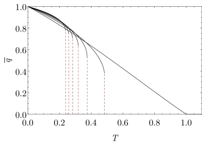
As a comparison, in Fig. 1, we reported the solutions of the self-consistency equations (52) for (solid curves), and the critical temperatures as predicted by the system (53) (dashed lines).
5 Application to Dense Associative Memories
Going beyond the pure spin-glass case, in this Section we will approach the DAMs that are the main focus of this work.
Definition 7.
Let be the generic point in the configuration space of the system. Given random patterns each made of i.i.d. binary entries drawn with equal probability , the Hamiltonian of the -th order DAM is
| (54) |
Remark 6.
The normalization factor ensures the linear extensivity of the Hamiltonian, in the volume of the network , i.e. .
As already stated in Sec. 1, DAMs with -order interactions are able to store at most a number of patterns , with baldi1987number ; bovier2001spin and, in the following, we will study the model in two different regimes, that is, setting finite and setting such that is finite, corresponding to, respectively, a simple and a complex scenario.
5.1 Low storage
Let us start the analysis of the network in a low-load regime, storing a finite number of patterns. Again, the goal is to use interpolation techniques and derive PDEs equations able to describe the thermodynamics of the system. To do this, let start by defining
Definition 8.
The order parameters used to describe the macroscopic behavior of the model are the so-called Mattis magnetizations, defined as
| (55) |
measuring the overlap between the network configuration and the stored patterns.
Remark 7.
The Hamilton function (54) in terms of the Mattis magnetizations is
Next, we define the basic objects of our investigations within the interpolating framework.
Definition 9.
Given , the spacetime Guerra’s interpolating partition function for the DAM model (in the low-load regime) reads as
| (56) | |||||
| (57) |
Remark 8.
Clearly, the spacetime Guerra’s interpolating partition function recovers the one related to the DAM by setting and .
Remark 9.
We recall that, for the CW model, the Guerra mechanical analogy consists in interpreting the statistical pressure as the Burgers hierarchy describing the motion of viscid non-linear waves in -dimensional space. In the case of the DAMs, we have Mattis magnetizations, and the dual mechanical system describes non-linear waves travelling in a -dimensional space.
Definition 10.
For each configuration of the system, the Boltzmann factor corresponding to the partition function (56) is
| (58) |
Proposition 3.
The first-order spacetime derivatives of the Guerra intensive pressure associated to the partition function (56) read as
| (59) | |||||
| (60) |
where .
Proof.
Recalling the definition of the intensive pressure , along with eq. 58, the proof follows straightforward computations. The temporal derivative reads
while the spatial derivative reads
∎
Proposition 4.
The higher (non-centered) momenta of the Mattis magnetizations are realized as
| (61) |
for each integer .
Proof.
We start by computing the spatial derivative of the Mattis magnetizations expectation value:
In particular, for , we have
Expressing the higher order moment in terms of the other quantities, we reach the thesis. ∎
By calling , we can express all in terms of for each . Indeed
| (62) |
To simplify the notation, we define the operator .
Theorem 2.
The expectation value of the Mattis magnetizations of the interpolated DAM model (9) satisfies the non-linear evolutive equations
| (63) |
Proof.
First, we put in (62), so that
Now, recall that and , thus
Taking the derivative , commuting and and recalling that , we directly reach the thesis. ∎
Lemma 3.
The evolutive equations (63) can be linearized by means of the Cole-Hopf transform.
Proof.
To proof our assertion, we use the basic identities
Performing the multi-dimensional Cole-Hopf transform , we have
and using the previous properties we have
Setting the argument of the spatial derivative to zero and assuming , we have
∎
Remark 10.
In the proof, the function is nothing but Guerra’s interpolating partition function, as can be understood by comparing the definitions and . Indeed, by computing the derivatives of the partition function we easily get
A direct comparison shows that Guerra’s interpolating partition function satisfies the same differential equation of the potential.
Remark 11.
The case corresponds to the -spin CW model treated in fachechi2021pde . Indeed, the partition function of the system can be handled as
where we used the invariance of the partition function under the transformation . In this particular case we recover the Burgers hierarchy with viscosity parameter : calling and , the family (63) reduces to
Within this framework, we generate multi-dimensional generalization of Burgers hierarchy, see Appendix B for further details and examples.
5.2 High-storage
Here we will study the -spin DAMs in the high-load regime for even , which now behaves as a complex system with global non-trivial properties. Let us start by observing that, in this case, the partition function related to the Hamiltonian (54) can also be written in the following form111Notice the little abuse of notation in the expression : in the subscript, ismeant as the ratio by-passing the thermodynamic limit:
| (64) |
and, by Hubbard-Stratonovich transforming, we get
| (65) |
Here, we used the index rather than in order to distinguish between the partition function of low and high storage regimes.
Remark 12.
As standard in statistical mechanics of (complex) neural networks, we will assume that a single pattern is candidate to be retrieved, say . Under this assumption, we can treat separately the Mattis magnetization corresponding to the recalled pattern from those associated to non-retrieved ones.
Definition 11.
Given , the spacetime Guerra’s interpolating partition function for the DAM model (in the high storage regime) reads as
| (66) | |||||
where .
Remark 13.
Clearly, the partition function of the original DAM model (65) is recovered by setting and .
In the case under consideration, the Boltzmann average w.r.t. the interpolating measure is
| (68) |
where is a generic observables in the configuration space of the system, and is the generalized Boltzmann factor for the -spin model defined as
As we said in Sec. 1, the high storage regime of associative neural networks exhibits both ferromagnetic and spin-glass features. Thus, besides the usual Mattis magnetisations, we need the overlap for the two sets of relevant variables in the integral formulation of the partition function (65):
Definition 12.
The order parameters used to describe the macroscopic behavior of the model are the overlap (already defined in (8) and used to quantify the retrieval capability of the network), the replica overlap in the variables
| (69) |
and the replica overlap in the ’s variables
| (70) |
With all these ingredients at our hand, we now move to the formulation of the PDE duality of DAMs in the high-storage limit.
Definition 13.
For all even , Guerra’s action functional is defined as
| (71) |
Lemma 4.
The partial derivatives of Guerra’s action can be expressed in terms of the generalized expectations of the order parameters as
| (72) |
The computation of the spacetime derivatives is pretty lengthy but straightforward. We report the computation of the derivatives in Appendix C.
In order to derive differential identities for the expectation values of the order parameters, we need to compute the spatial derivatives of a generic function of two replicas .
Proposition 5.
Let and be the configurations of the 2-replicated system. Then
| (73) |
| (74) |
and
| (75) |
The complete proof is given in Appendix D.
Corollary 3.
For all , the following equalities holds
| (76) |
Proof.
Also in this case, we will work under the RS assumption in order to simplify the computations by neglecting the fluctuations of the order parameters w.r.t. their expectation values.
Proposition 6.
The following equalities holds
| (77) | |||||
| (78) |
where collects the terms involving the fluctuations of the order parameters, and thus vanishes in the limit and under the RS assumption.
Proof.
To simplify the notation, we will drop the subscript from the quenched averages. The derivation of (77) iterating the property (75) with . Let us now observe that
and
where , and collect the contributions involving the fluctuations. Then, recalling eq.(76), we can write
where and we used following from the invariance under replica labelling. The previous equation can be thus written in the following way
| (79) |
Iterating the procedure, we get
| (80) |
where collects all the terms involving the rests of previous expansions (and thus vanishes in the limit and under the RS assumption). Then, by imposing we get the thesis. ∎
Now we can use all the information obtained to build a PDE that can describe the thermodynamics of the DAM models. Indeed, recalling the temporal derivative of the Guerra’s action (72) and using the result obtained in Prop. 6, we have
| (81) |
Finally, taking the spatial derivatives of this expression and denoting , we have
| (82) |
The l.h.s. of the system of PDEs constitute the 3+1-dimensional DAM generalization of the Burgers hierarchy structure. Similarly to the Derrida model case, at finite we have a source term on the r.h.s. which vanishes in the limit under the RS assumption of the order parameters. In this case, we can analyse the thermodynamic limit and describe the equilibrium dynamics of the model.
Theorem 3.
The high-storage regime for the DAM models under the RS assumption in the thermodynamic limit can be described by the following system of partial differential equations:
| (83) |
with the initial conditions
| (84) |
where is the Gaussian average over the variable .
Proof.
First, let us call
the expectation values of the order parameters in the thermodynamic limit. Taking in (82) and recalling that the source contributions vanish in this limit under the RS assumption, we arrive at the PDE system (83). Let us now find the initial conditions (84). To do this we start calculating the interpolating partition function in
By using the definition of the interpolating statistical pressure (4), we see that
where we used the fact that the are i.i.d. random variables and for all . Now, recalling Eq. (71), we can straightforwardly derive the initial condition for the order parameters according to (72). First
| (85) |
Analogously, we have
| (86) |
Finally
| (87) |
This concludes the proof. ∎
Proposition 7.
The system of PDEs (83) can be rewritten in a non-linear wave equation as
| (88) |
where is the vector of the order parameters and is the effective velocity.
Proof.
We prove the equation (88) for the first component, as the others follow accordingly. Let us define the function , so that the PDE for the order parameter can be rewritten as
The -derivative of the function is straightforwardly computed:
Now
In the same way
With these results, we have
This leads to
∎
Proposition 8.
The equilibrium dynamics of the DAM models is given by the set of self-consistency equations
| (89) |
where .
Proof.
In order to proof our assertion, we use the vector PDE (88), whose solution can be given in implicit form as
where is the initial profile given by the conditions (84). For the first component, we have
| (90) |
Analogously,
| (91) |
Finally, if , we have
| (92) |
while, for with , the same order parameter satisfies the self-consistency equation
| (93) |
Recalling that the thermodynamics of the DAM models is reproduced when and , we easily get the thesis. ∎
Remark 14.
We stress that the self-consistency equations in Prop. 8 are in agreement with those obtained by Gardner in gardner1987 by means of replica trick.
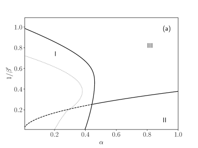
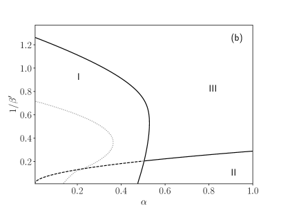
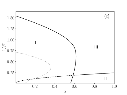
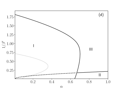
By solving these self-consistency equations (89) numerically by a fixed-point method for a given and tuning the parameters and , we obtain the phase diagrams shown in Fig. 2. As expected, the diagrams exhibit the existence of three different regions:
-
•
For high levels of noise , no matter the value of storage , the only stable solution is given by , , thus the system is ergodic (III);
-
•
At lower temperatures and with relatively high load, the system exhibits spin-glass behaviors (II), and the solution is characterized by and ;
-
•
For relatively small values of and , we have and the system is located in the retrieval phase (I). In this situation, the system behaves as an associative neural network performing spontaneously pattern recognition. In particular, we can see that the retrieval region observed for values of and relatively small can be further split in a pure retrieval region , where pure states are global minima for the free energy, and in a mixed retrieval region, where pure states are local minima, yet their attraction basin is large enough for the system to end there if properly stimulated.
Thus, by increasing we need to afford higher costs in terms of resources, since the number of connection weights to be properly set grows as , but we also have a reward on a coarse scale, since the number of storable patterns grows as , as well as on a fine scale, since the critical load is also increasing with .
6 Conclusions
In this work we focused on DAMs, that are neural-network models widely used for pattern recognition tasks and characterized by high-order (higher than quadratic) interactions between the constituting neurons. Extensive empirical evidence has shown that these models significantly outperform non-dense networks (displaying only quadratic interactions), especially as for the ability to correctly recognize adversarial or extremely noisy examples Krotov2016DenseAM ; Krotov2018DAMS ; AABCF-PRL2020 ; AD-EPJ2020 hence making these models particularly suitable for detecting and cope with malicious attacks. From the theoretical side, results are sparse and mainly based on the possibility of recasting these networks as spin-glass-like models with spins interacting -wisely; these models can, in turn, be effectively faced by tools stemming from the statistical mechanics of disordered systems (e.g., Bovier-JPA1994 ; AABF-NN2020 ). Here, we pave this way and develop analytical techniques for their investigation. More precisely, we translate the original statistical-mechanical problem into an analytical-mechanical one where control parameters play as spacetime coordinates, the free-energy plays as an action and the macroscopic observables that assess whether the system can be used for pattern recognition tasks play as effective velocities and are shown to fulfil a set of nonlinear partial differential equations. In this framework, transitions from different regimes (e.g., from a region in the control parameter space where the system performs correctly and another one where information processing capabilities are lost) appear as the emergence of shock waves.
A main advantage of this route is that it allows for rigorous investigations in a field where most knowledge is based on (pseudo) heuristic approaches, with a wide set of already available methods and strategies to rely upon. Further, by bridging two different perspectives, the statistical-mechanics and the analytical one, we anticipate a cross-fertilization that may lead to a deeper comprehension of the system subtle mechanisms and ultimately progress in the development of a complete theory for (deep) machine learning.
Acknowledgments
E.A. and A.F. would like to thank A. Moro for useful discussions. The authors acknowledge Sapienza University of Rome for financial support (RM120172B8066CB0, RM12117A8590B3FA, AR12117A623B0114).
Appendix A Proof of Lemma 1
Proof.
First of all, we compute the temporal derivative:
| (94) |
Here, we can use the Wick-Isserlis theorem for normally distributed random variables, ensuring that for each function of the quenched disorder . Thus
| (95) |
The non-trivial contribution in the round brackets in the last equality can be expressed in terms of the overlap order parameter. Indeed
| (96) |
where are the replica indices. Now, using Rem. 2, in the thermodynamic the following equality holds:
| (97) |
Concerning the spatial derivative, we proceed in the same way:
| (98) |
Also in this case, we express , thus
| (99) |
By simply exploiting Def. 6 and the Rem.2 we get the thesis. ∎
Appendix B Particular cases of low storage DAMs
In this Appendix, having clear the equations describing the general case of the DAM models in the low storage regime, we will study two special cases namely the standard case where and the more complex case with . In particular, we will observe that these two cases can be described by the Burgers and Sharma-Tasso-Olver equations in a -dimensional space, respectively. To start this study, however, we first need the following definition and Lemma.
Lemma 5.
For all , we have
-
1.
;
-
2.
where is the usual commutator.
Proof.
The proof of the statement works by direct computation. Indeed:
Since the field is conservative, i.e. , we have
meaning that Let as now prove the property In this case the proof works by exploiting the property (from which it follows also ) and the definition . Indeed
By rearranging the equality we easily get the thesis. ∎
From the previous lemma we can then prove the following two propositions
Proposition 9.
In the case with a generic finite , the evolutive equations (63) reduces to the multidimensional Burgers equation.
Proof.
Proposition 10.
In the case (and generic ), the evolutive equations (63) reduces to the multidimensional Sharma-Tasso-Olver (STO) equation olver1977evolution ; tasso1976cole .
Appendix C Proof of Lemma 4
Proof.
We prove the equality for the -derivative of the Guerra’s action, as the others follow with similar calculations. To do this, we first compute the temporal derivative of the interpolating statistical pressure:
Since non-retrieved patterns constitutes a noise contribution to the system dynamics, we can assume - with standard arguments about the universality of noise Genovese_2012 ; Agliari_2019 - that the whole product is Gaussian-distributed as long as and . Thus, we can apply the Wick-Isserlis theorem on the second contribution to get
where we used the definitions of the overlap order parameters (69) and (70). Recalling that , we finally get the result. ∎
Appendix D Proof of Proposition 5
Proof.
We only prove the equation (73), the other one can be obtained in an analogous way. We will denote for simplicity of notation with . Thus
| (101) |
where in the last line we used the Wick-Isserlis theorem. Now, it is simple to see that
| (102) |
and
| (103) |
By substituting and into we get
Recalling that we can write
| (104) |
thus obtaining Eq. (73). ∎
References
- (1) Y. LeCun, Y. Bengio, and G. Hinton, “Deep learning,” Nature, vol. 521, no. 7553, pp. 436–444, 2015.
- (2) J. Schmidhuber, “Deep learning in neural networks: an overview,” Neural Networks, vol. 61, pp. 85–117, 2015.
- (3) M. Mézard, G. Parisi, and M. A. Virasoro, Spin glass theory and beyond: An Introduction to the Replica Method and Its Applications, vol. 9. World Scientific Publishing Company, 1987.
- (4) D. Sherrington and S. Kirkpatrick, “Solvable model of a spin-glass,” Physical Review Letters, vol. 35, no. 26, p. 1792, 1975.
- (5) G. Parisi, “Toward a mean field theory for spin glasses,” Physics Letters A, vol. 73, no. 3, pp. 203–205, 1979.
- (6) G. Parisi, “Infinite number of order parameters for spin-glasses,” Physical Review Letters, vol. 43, no. 23, p. 1754, 1979.
- (7) G. Parisi, “The order parameter for spin glasses: a function on the interval 0-1,” Journal of Physics A: Mathematical and General, vol. 13, no. 3, p. 1101, 1980.
- (8) G. Parisi, “A sequence of approximated solutions to the SK model for spin glasses,” Journal of Physics A: Mathematical and General, vol. 13, no. 4, p. L115, 1980.
- (9) M. Mézard, G. Parisi, N. Sourlas, G. Toulouse, and M. Virasoro, “Replica symmetry breaking and the nature of the spin glass phase,” Journal de Physique, vol. 45, no. 5, pp. 843–854, 1984.
- (10) F. Guerra, “Broken replica symmetry bounds in the mean field spin glass model,” Communications in Mathematical Physics, vol. 233, no. 1, pp. 1–12, 2003.
- (11) S. Ghirlanda and F. Guerra, “General properties of overlap probability distributions in disordered spin systems. Towards Parisi ultrametricity,” Journal of Physics A: Mathematical and General, vol. 31, no. 46, p. 9149, 1998.
- (12) M. Talagrand, “Replica symmetry breaking and exponential inequalities for the Sherrington-Kirkpatrick model,” The Annals of Probability, vol. 28, no. 3, pp. 1018–1062, 2000.
- (13) D. Panchenko, “A connection between the Ghirlanda–Guerra identities and ultrametricity,” The Annals of Probability, vol. 38, no. 1, pp. 327–347, 2010.
- (14) D. Panchenko, “Ghirlanda–Guerra identities and ultrametricity: An elementary proof in the discrete case,” Comptes Rendus Mathematique, vol. 349, no. 13-14, pp. 813–816, 2011.
- (15) D. Panchenko, “The parisi ultrametricity conjecture,” Annals of Mathematics, pp. 383–393, 2013.
- (16) D. J. Amit, H. Gutfreund, and H. Sompolinsky, “Storing infinite numbers of patterns in a spin-glass model of neural networks,” Physical Review Letters, vol. 55, no. 14, p. 1530, 1985.
- (17) J. J. Hopfield, “Neural networks and physical systems with emergent collective computational abilities,” Proceedings of the national academy of sciences, vol. 79, no. 8, pp. 2554–2558, 1982.
- (18) L. A. Pastur and A. L. Figotin, “Exactly soluble model of a spin glass,” Journal of Low Temperature Physics, vol. 3, no. 6, pp. 378–383, 1977.
- (19) D. Krotov and J. J. Hopfield, “Dense associative memory for pattern recognition,” Advances in neural information processing systems, vol. 29, 2016.
- (20) D. Krotov and J. Hopfield, “Dense associative memory is robust to adversarial inputs,” Neural computation, vol. 30, no. 12, pp. 3151–3167, 2018.
- (21) E. Agliari and G. De Marzo, “Tolerance versus synaptic noise in dense associative memories,” The European Physical Journal Plus, vol. 135, no. 11, pp. 1–22, 2020.
- (22) P. Baldi and S. S. Venkatesh, “Number of stable points for spin-glasses and neural networks of higher orders,” Physical Review Letters, vol. 58, no. 9, p. 913, 1987.
- (23) A. Bovier and B. Niederhauser, “The spin-glass phase-transition in the Hopfield model with -spin interactions,” Mathematical Physics and Mathematics, 2001.
- (24) H. Steffan and R. Kühn, “Replica symmetry breaking in attractor neural network models,” Zeitschrift für Physik B Condensed Matter, vol. 95, no. 2, pp. 249–260, 1994.
- (25) T. Tanaka, “Moment problem in replica method,” Interdisciplinary information sciences, vol. 13, no. 1, pp. 17–23, 2007.
- (26) F. Guerra, “Sum rules for the free energy in the mean field spin glass model,” Fields Institute Communications, vol. 30, no. 11, 2001.
- (27) E. Agliari, A. Barra, R. Burioni, and A. Di Biasio, “Notes on the p-spin glass studied via Hamilton-Jacobi and smooth-cavity techniques,” Journal of Mathematical Physics, vol. 53, no. 6, p. 063304, 2012.
- (28) A. Barra, G. Dal Ferraro, and D. Tantari, “Mean field spin glasses treated with PDE techniques,” The European Physical Journal B, vol. 86, no. 7, pp. 1–10, 2013.
- (29) A. Barra, “The mean field ising model trough interpolating techniques,” Journal of Statistical Physics, vol. 132, no. 5, pp. 787–809, 2008.
- (30) A. Barra, A. Di Biasio, and F. Guerra, “Replica symmetry breaking in mean-field spin glasses through the Hamilton–Jacobi technique,” Journal of Statistical Mechanics: Theory and Experiment, vol. 2010, no. 09, p. P09006, 2010.
- (31) A. Barra, A. Di Lorenzo, F. Guerra, and A. Moro, “On quantum and relativistic mechanical analogues in mean-field spin models,” Proceedings of the Royal Society A: Mathematical, Physical and Engineering Sciences, vol. 470, no. 2172, p. 20140589, 2014.
- (32) G. De Matteis, F. Giglio, and A. Moro, “Exact equations of state for nematics,” Annals of Physics, vol. 396, pp. 386–396, 2018.
- (33) E. Agliari, D. Migliozzi, and D. Tantari, “Non-convex multi-species Hopfield models,” Journal of Statistical Physics, vol. 172, no. 5, pp. 1247–1269, 2018.
- (34) P. Lorenzoni and A. Moro, “Exact analysis of phase transitions in mean-field Potts models,” Physical Review E, vol. 100, no. 2, p. 022103, 2019.
- (35) E. Agliari, A. Barra, and M. Notarnicola, “The relativistic Hopfield network: Rigorous results,” Journal of Mathematical Physics, vol. 60, no. 3, p. 033302, 2019.
- (36) A. Fachechi, “PDE/statistical mechanics duality: Relation between Guerra’s interpolated -spin ferromagnets and the Burgers hierarchy,” Journal of Statistical Physics, vol. 183, no. 1, pp. 1–28, 2021.
- (37) E. Agliari, L. Albanese, F. Alemanno, and A. Fachechi, “A transport equation approach for deep neural networks with quenched random weights,” Journal of Physics A: Mathematical and Theoretical, vol. 54, no. 50, p. 505004, 2021.
- (38) A. Barra and A. Moro, “Exact solution of the Van der Waals model in the critical region,” Annals of Physics, vol. 359, pp. 290–299, 2015.
- (39) G. De Nittis and A. Moro, “Thermodynamic phase transitions and shock singularities,” Proceedings of the Royal Society A: Mathematical, Physical and Engineering Sciences, vol. 468, no. 2139, pp. 701–719, 2012.
- (40) F. Giglio, G. Landolfi, and A. Moro, “Integrable extended Van der Waals model,” Physica D: Nonlinear Phenomena, vol. 333, pp. 293–300, 2016.
- (41) A. Moro, “Shock dynamics of phase diagrams,” Annals of Physics, vol. 343, pp. 49–60, 2014.
- (42) B. Derrida, “Random-energy model: An exactly solvable model of disordered systems,” Physical Review B, vol. 24, no. 5, p. 2613, 1981.
- (43) L. Pastur and M. Shcherbina, “Absence of self-averaging of the order parameter in the Sherrington-Kirkpatrick model,” Journal of Statistical Physics, vol. 62, no. 1, pp. 1–19, 1991.
- (44) A. Bovier, “Self-averaging in a class of generalized Hopfield models,” Journal of Physics A: Mathematical and General, vol. 27, no. 21, p. 7069, 1994.
- (45) D. J. Amit, Modeling brain function: The world of attractor neural networks. Cambridge university press, 1989.
- (46) E. Agliari, A. Barra, P. Sollich, and L. Zdeborová, “Machine learning and statistical physics: preface,” Journal of Physics A: Mathematical and Theoretical, vol. 53, p. 500401, 2020.
- (47) E. Agliari, L. Albanese, A. Barra, and G. Ottaviani, “Replica symmetry breaking in neural networks: a few steps toward rigorous results,” Journal of Physics A: Mathematical and Theoretical, vol. 53, no. 41, p. 415005, 2020.
- (48) L. Albanese, F. Alemanno, A. Alessandrelli, and A. Barra, “Replica symmetry breaking in dense neural networks,” arXiv preprint arXiv:2111.12997, 2021.
- (49) E. Gardner, “Multiconnected neural network models,” Journal of Physics A: Mathematical and General, vol. 20, no. 11, p. 3453, 1987.
- (50) E. Agliari, F. Alemanno, A. Barra, M. Centonze, and A. Fachechi, “Neural networks with a redundant representation: detecting the undetectable,” Physical Review Letters, vol. 124, no. 2, p. 028301, 2020.
- (51) E. Agliari, F. Alemanno, A. Barra, and A. Fachechi, “Generalized Guerra’s interpolation schemes for dense associative neural networks,” Neural Networks, vol. 128, pp. 254–267, 2020.
- (52) P. J. Olver, “Evolution equations possessing infinitely many symmetries,” Journal of Mathematical Physics, vol. 18, no. 6, pp. 1212–1215, 1977.
- (53) H. Tasso, “Cole’s ansatz and extensions of Burgers’ equation,” tech. rep., Max-Planck-Institut für Plasmaphysik, 1976.
- (54) G. Genovese, “Universality in bipartite mean field spin glasses,” Journal of Mathematical Physics, vol. 53, no. 12, p. 123304, 2012.
- (55) E. Agliari, A. Barra, and B. Tirozzi, “Free energies of Boltzmann machines: self-averaging, annealed and replica symmetric approximations in the thermodynamic limit,” Journal of Statistical Mechanics: Theory and Experiment, vol. 2019, no. 3, p. 033301, 2019.